3.7. Some Examples and Illustrations
Example 1. Prediction of calcium contents.
This dataset was considered in [
22]. The
PID developed here, along with the
PID [
22] and
PID [
20], was applied using data on 73 women involving one set of predictors
(Age, Weight, Height), another set of two predictors
(diameter of os calcis, diameter of radius and ulna), and target
(calcium content of heel and forearm). The following results were obtained.
| PID | | Unq1 | Unq2 | Shd | Syn |
| | 0.2408 | 0.3581 | 0.0304 | 0.0728 | 0.1904 |
| | | 0.4077 | 0.0800 | 0.0232 | 0.1408 |
| | | 0.3277 | 0 | 0.1032 | 0.2209 |
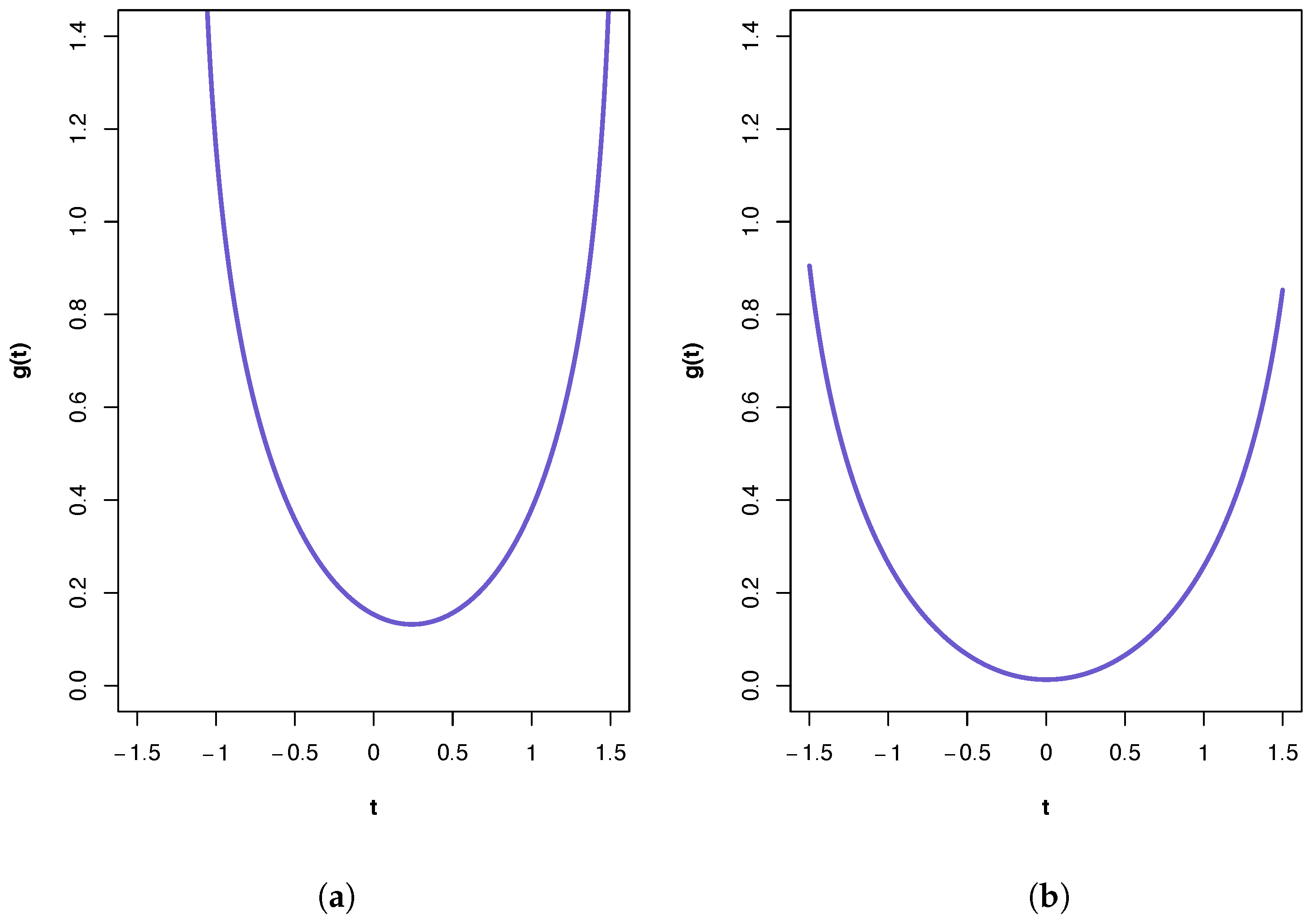
A plot of the ‘synergy’ function
is shown in
Figure 2a. All three PIDs indicate the presence of synergy and a large component of unique information due to the variables in
. The
PID suggests the transmission of more of the joint mutual information as shared and synergistic information and correspondingly less unique information due to either source vector than does the
PID. This is true also for the results from the
PID, but it has higher values for synergistic and shared information and a lower value for Unq1 than those produced by the
PID. It was shown in [
22] that pdf
p in manifold M provides a better fit to these data than any of the submanifold distributions. This pdf contains pairwise cross-correlation between the vectors
and
, and between
and
. Hence, it is no surprise to find that a relatively large Unq1 component. One might also anticipate a large value for Unq2. That this is not the case is explained, at least partly, by the presence of unique information asymmetry, in that the mutual information between
and
(0.4309) is much larger than that between
and
(0.1032) and also bearing in mind the constraints imposed by (6)–(10).
The PIDs were also computed with the same
and
but taking
to be another set of four predictors (surface area, strength of forearm, strength of leg, area of os calcis). The following results were obtained.
| PID | | Unq1 | Unq2 | Shd | Syn |
| 0.0027 | 0.3522 | 0.0000 | 0.0787 | 0.0186 |
| | | 0.3708 | 0.0186 | 0.0601 | 0 |
| | | 0.3522 | 0 | 0.0787 | 0.0186 |
A plot of the ‘synergy’ function
is shown in
Figure 2b. In this case, the PIDs obtained from all three methods are very similar, with the main component being unique information due to the variables in
. The PIDs indicate almost zero synergy and almost zero unique information due to the variables in
. In [
22], it was shown that the best of the pdfs is
associated with submanifold
. If this model were to hold exactly, then a PID must have Syn and Unq2 components that are equal to zero. Therefore, all three PIDs perform very well here, and the fact that the Unq1 component is much larger than the Shd component is due to unique information asymmetry, since the mutual information between
and
is only 0.0787. In this dataset, the
PID suggests the transmission just a little more of the joint mutual information as shared and synergistic information and correspondingly less unique information due to either source vector than does the
PID. The
and
PIDs produce identical results (to 4 d.p.).
When working with real or simulated data, it is important to use the correct covariance matrix. In order to use the results given in Proposition 1, it is essential that the input covariance matrix has the structure of
, as given in (12). Further detail is provided in
Appendix J.
Example 2. PID expectations and exact results.
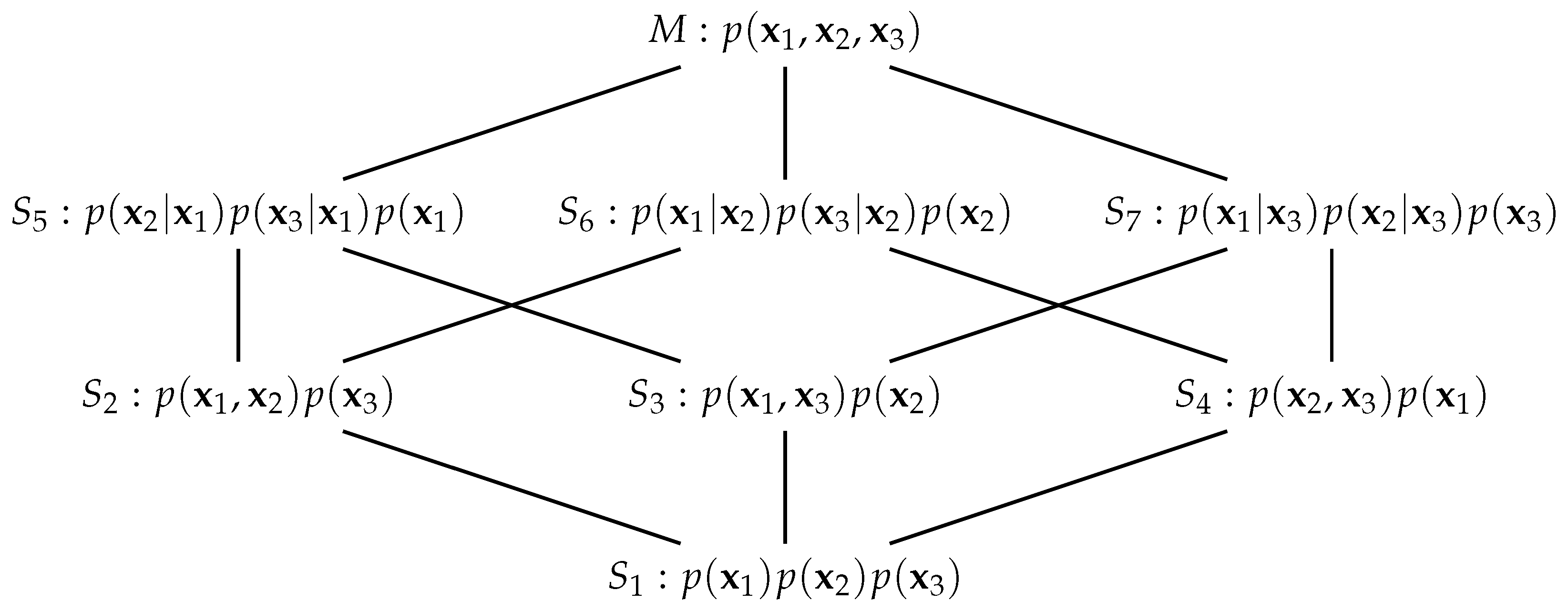
Since there is no way to know the true PID for any given dataset it is useful to consider situations under which some values of the PID components can be predicted, and this approach has been used in developments of the topic. Here, we consider such expectations provided by the pdfs associated with the submanifolds
, defined in
Figure 1. In submanifold
, the source
is independent of both the other source
and the target
. Hence, we expect only unique information due to source
to be transmitted. Submanifold
is similar but we expect only unique information due to source
to be transmitted. In manifold
,
and
are conditionally independent given a value for
. Hence, from (9), we expect the Unq2 and Syn components to be zero. Similarly, for
, we expect the Unq1 and Syn components to be equal to zero, by (8). On submanifold
, the sources
are conditionally independent given a value for the target
(which does not mean that the sources are marginally independent). Since the target
interacts with both source vectors, one might expect some shared information as well as unique information from both sources, and also perhaps some synergy. Here, from (11), the interaction information must be negative or zero, and so we can expect to see transmission of more shared information than synergy.
We will examine these expectations by using the following multivariate Gaussian distribution (which was used in [
22]). The matrices
are given an equi-cross-correlation structure in which all the entries are equal within each matrix:
where
denote here the constant cross correlations within each matrix and
denotes an n-dimensional vector whose entries are each equal to unity.
The values of
are taken to be
, with
,
. Covariance matrices for pdfs
were computed using the results in
Table 1. Thus, we have the exact covariance matrices which can be fed into the
,
and
algorithms. The PID results are displayed in
Table 2.
From
Table 2, we see that all three PIDs meet the expectations exactly for pdfs
, with only unique information transmitted when the pdfs
, are true, respectively, and zero unique for the relevant component and zero synergy when the models
are true, respectively. When model
is the true model, we find that the
and
PIDs produce virtually identical results: the joint mutual information is transmitted almost entirely as synergistic information. The
PID is slightly different, with less unique information transmitted about the variables in
, and more shared and synergistic information transmitted than with the other two PIDs. The PIDs produce very different results for pdf
, although, as expected, they do express more shared information than synergy. When this model is satisfied,
sets the synergy to 0, even if there is no compelling reason to support this. This curiosity is mentioned and illustrated in [
22]. On the other hand, the
PID suggests that each of the four components contributes to the transmission of the joint mutual information, with unique information due to
and shared information making more of a contribution than the other two components. The
PID transmits a higher percentage of the joint information as shared and synergistic information, and a smaller percentage due to the variables in
, than is found with
; these differences are much stronger when comparison is made with the corresponding
components. As with model
p, it appears that the setting of the Unq1 component in
to zero has been translated into its percentage being subtracted from the Unq2 component and added to both the Shd and Syn components in
to produce
.
Example 3. Some simulations.
Taking the same values of
and
as in the previous example, a small simulation study was conducted. From each of the pdfs,
, a simple random sample of size 1000 was generated from the 10-dimensional distribution, a covariance matrix estimated from the data and the
,
and
algorithms were applied. This procedure was repeated 1000 times. In order to make the PID results from the sample of 1000 datasets comparable each PID was normalized by dividing each of its components by the joint mutual information; see (10). A summary of the results is provided in
Table 3. We focus here on the comparison of
and
, and also
and
, since
has been compared with
for Gaussian systems [
22].
For pdf
p, the
and
PIDs produce very similar results in terms of both median and range, and the median results are very close indeed to the corresponding exact values in
Table 2. For pdf
, the differences between the PID components found in
Table 2 persist here although each PID, respectively, produces median values of their components that are close to the exact results in
Table 2. For the other four pdfs, there are some small but interesting differences among the results produced by the two PID methods. The
method has higher median values for synergy and shared information than for the unique information, when compared against the corresponding exact values in
Table 2. In particular, the values of unique information given by
are much lower than expected for pdfs
, and the levels of synergy are larger than expected particularly for pdfs
and
. On the other hand, the
PID tends to have larger values for the unique information, and lower values for synergy, especially for datasets generated from pdfs
,
and
. For models
,
has median values of synergy that are closer to the corresponding exact values than those produced by
. The suggestion that the
method can produce more synergy and shared information than the
method, given the same dataset, is supported by the fact that for all the pdfs and all 6000 datasets considered, the
method produced greater levels of synergy and shared information and smaller values of the unique information in
every dataset. This raises a question of whether such a finding is generally the case and whether there is this type of a systematic difference between the methods. In the case of scalar variables, it is easy to derive general analytic formulae for the
PID components and such a systematic difference is present in this case.
The
and
PIDs produce similar results for the datasets generated from pdf
p, although the
PID suggests the transmission of more shared and synergistic information and less unique information than does
. For pdf
, the differences between the PID results are much more dramatic, with the
PID allocating an additional 15% of the joint mutual information to be shared and the synergistic information, and correspondingly 15% less of the unique information. Both methods produce almost identical summary statistics on the datasets generated from pdfs
. Since the same patterns are present for all four distributions, we discuss the results for pdf
as an exemplar and compare them with the corresponding exact values in
Table 2. The results for component Unq1 show that both methods produce an underestimate of approximately 7%, on average, of the joint mutual information. The median values of Unq2 are close to those expected. The underestimates on the Unq1 component are coupled with overestimates, on average, for the shared and synergistic components; they are 2.6% and 4.3%, respectively, with the
method, and 3.1% and 4.7%, respectively, with
.
As to be expected with percentage data, the variation in results for each component tends to be larger for values that are not extreme and much smaller for the extreme values. Also, the optimal values of
are shown in
Table 3. They were all found to be in the range [0, 1], except for 202 of the datasets generated from pdf
or
.


