
Angular Distributions of Emitted Electrons in the Two-Neutrino ββ Decay


1
Faculty of Mathematics, Physics and Informatics, Comenius University in Bratislava, 842 48 Bratislava, Slovakia
2
International Centre for Advanced Training and Research in Physics, P.O. Box MG12, 077125 Măgurele, Romania
3
“Horia Hulubei” National Institute of Physics and Nuclear Engineering, 30 Reactorului, POB MG-6, RO-077125 Bucharest-Măgurele, Romania
4
Dzhelepov Laboratory of Nuclear Problems, Joint Institute for Nuclear Research, 141980 Dubna, Russia
5
Bogoliubov Laboratory of Theoretical Physics, Joint Institute for Nuclear Research, 141980 Dubna, Russia
6
Institute of Experimental and Applied Physics, Czech Technical University in Prague, 110 00 Prague, Czech Republic
*
Author to whom correspondence should be addressed.
Universe 2021, 7(5), 147; https://doi.org/10.3390/universe7050147
Submission received: 14 April 2021
/
Revised: 10 May 2021
/
Accepted: 11 May 2021
/
Published: 14 May 2021
(This article belongs to the Special Issue Nuclear Issues for Neutrino Physics)
Abstract
:The two-neutrino double-beta decay (-decay) process is attracting more and more attention of the physics community due to its potential to explain nuclear structure aspects of involved atomic nuclei and to constrain new (beyond the Standard model) physics scenarios. Topics of interest are energy and angular distributions of the emitted electrons, which might allow the deduction of valuable information about fundamental properties and interactions of neutrinos once a new generation of the double-beta decay experiments will be realized. These tasks require an improved theoretical description of the -decay differential decay rates, which is presented. The dependence of the denominators in nuclear matrix elements on lepton energies is taken into account via the Taylor expansion. Both the Fermi and Gamow-Teller matrix elements are considered. For nuclei of experimental interest, relevant phase-space factors are calculated by using exact Dirac wave functions with finite nuclear size and electron screening. The uncertainty of the angular correlation factor on nuclear structure parameters is discussed. It is emphasized that the effective axial-vector coupling constant can be determined more reliably by accurately measuring the angular correlation factor.
1. Introduction
There is an increased interest in the two-neutrino double-beta decay (-decay) mode with an emission of two electrons and two antineutrinos
which was suggested by Maria Goeppert-Mayer in 1935 [1]. The -decay is the second order process of weak interaction fully consistent with the Standard model (SM) of particle physics, where two neutrons are simultaneously transformed into two protons inside an atomic nucleus, and two pairs of electrons and antineutrinos are emitted. It is the rarest process measured so far in nature with a half-life above years. The first direct observation of this process dates back to 1987 [2]. Currently, the -decay has been observed in eleven even–even nuclei for transition to ground state and in two cases also for transition to the first excited state of the final nucleus [3].
Several next-generation double-beta experiments with a variety of suitable isotopes are in different stages of construction or preparation and planning. Their main goal is the observation of the neutrinoless double-beta decay (-decay), a double-beta decay mode violating the total lepton number, in which only two electrons are emitted. It would prove that neutrinos are Majorana particles (i.e., neutrinos are their own antiparticles), as most theories beyond SM requires. Besides the Majorana nature of the neutrino, valuable information on the origin of neutrino masses, violation of CP in the lepton sector and possible existence of sterile neutrinos is expected, as well.
An important by-product of these experimental searches will be a precise measurement of the -decay with high statistics. The study of this process is important on its own and represents a research program with many important questions waiting for the answers. The -decay provides insights into nuclear structure [4] of nuclear systems under consideration which can then be used in a reliable calculation of the nuclear matrix elements (NMEs) for -decay, necessary to extract the particle physics parameters responsible for the lepton number violation [5] or in fixing the effective value of the axial-vector coupling constant [6,7,8,9].
With the increasing statistics of the -decay, the possibility of exploring new physics beyond SM with this process becomes more and more reliable. The -decay can be, and it is used for the search of the right-handed neutrino interactions without having to assume their nature [10], the neutrino self-interactions [11], the sterile neutrinos with masses up to Q-value of the process [12], the bosonic neutrino component [13], the violation of the Lorentz invariance [14,15,16,17], the -decays with Majoron(s) emission [18,19] and the quadruple- decay [20].
A necessary condition to gain rich information about fundamental properties and interactions of neutrinos from the precisely measured differential characteristics of the -decay is that all atomic and nuclear structure physics aspects of this process are well understood. Recently, the theoretical description of the shape of single and summed electron energy distributions of the -decay has been significantly improved by taking into account the dependence on lepton energies from the energy denominators of nuclear matrix elements [6], which was commonly neglected. However, their importance was already manifested by the study of -decay energy and angular distributions within the framework of the Single State Dominance (SSD) versus Higher State Dominance (HSD) hypothesis in [21,22]. In this paper, the theoretical study of Ref. [6] is extended to analyze the angular correlations of outgoing electrons by considering both the Fermi and Gamow-Teller components of the -decay nuclear matrix elements. For nuclei of experimental interest, all phase-space factors are calculated by using exact Dirac wave functions with finite nuclear size and electron screening.
2. The Angular Distribution
The inverse half-life of the -decay transition to the ground state of the final nucleus is defined as
where is the decay rate. If the contribution of higher partial waves of electron and higher order terms of the nucleon current are neglected as they are strongly suppressed [23], the angular distribution of emitted electrons takes the form [10]
where
is the angular correlation factor and is the angle between the emitted electrons. The decay rates are given by
with
Here, ( is the Fermi constant and is the Cabbibo angle [24]) and is the mass of electron. , and (, ) are the energies of initial and final nuclei and electrons, respectively. and are radial components of electron wave functions evaluated at nuclear surface with radius R, which will be introduced in the following sections. and consist of products of the Fermi and Gamow-Teller nuclear matrix elements, which depend on lepton energies:
where
with
Here, , are the ground states of the initial and final even–even nuclei, respectively, and () are all possible states of the intermediate nucleus with angular momentum and parity () and energy (). The lepton energies enter in the factors
The maximal value of and is the half of Q value of the process (). For decay with energetically forbidden transition to intermediate nucleus () the quantity is always larger than half of the Q value.
The Fermi (Gamow-Teller) operator governing the matrix elements () given in Equation (10) is a generator of an isospin SU(2) (spin-isospin SU(4)) multiplet symmetry. In the case both isospin and spin-isospin symmetries would be exact in nuclei the -decay would be forbidden as ground states of initial and final nuclei would belong to different multiplets. Usually, it is assumed that the contribution from Fermi matrix elements to the -decay amplitude is negligibly small as the isospin is known to be a reasonable approximation in nuclei. The main contribution is due to Gamow-Teller matrix elements. This fact is partially confirmed by the nuclear structure studies, which are, however, model dependent. There is a question whether it is possible to prove experimentally the dominance of the Gamow-Teller over Fermi contribution in the -decay.
2.1. The Standard Approximation and the HSD Hypothesis
Commonly, the calculation of the -decay distributions and decay rate is simplified by neglecting in energy denominators of NME’s by which a separation of phase-space factors and NMEs is achieved. We get
where Fermi and Gamow-Teller matrix elements are given by
As a consequence of Equation (12) the angular correlation factor (see Equations (4) and (5)) is not affected by the nuclear structure as the dependence on and is eliminated.
We note that this approximation scheme is justified when the contribution from higher lying states (, ) of the intermediate nucleus to the -decay rate dominates over the low lying states. Such theoretical assumption is denoted as the higher state dominance (HSD) hypothesis. The experimental observation shows that Fermi strength distribution from the initial to the intermediate nucleus is concentrated to the Isobaric Analogue State region with excitation energy above 10 MeV, that is, the isospin symmetry prevents any significant fragmentation of the Fermi transition. Contrary, the Gamow-Teller strength distribution is fragmented over many daughter states covering a region of Gamow-Teller resonance and a region of low-lying states of the intermediate nucleus. Thus, the HSD assumption is justified for Fermi matrix elements and it is an open question whether transitions through low-lying or higher-lying (region of the GT resonance) states of the intermediate nucleus give the main contribution to , or whether there is a mutual cancellation of these contributions.
2.2. The Angular Distribution within the SSD Hypothesis
A long time ago, it was proposed by Abad et al. [25] that the -decay is governed by the Gamow-Teller transitions connecting the ground states of initial (A,Z) and final (A,Z+2) even–even nuclei with the first state of the intermediate nucleus (A,Z+1). This assumption is known as the SSD hypothesis. Then, we have
and . In this case the normalized to the full width single and summed electron differential decay rates and the angular correlation factor are free of , but they are affected by the lepton energies incorporated in and the energy difference [21,22]. The experimental study of energy distributions performed for -decay of Se [26] and Mo [19] showed a clear preference for the SSD scenario over the HSD scenario. However, a better interpretation of experimental data requires an improved theoretical description the -decay process.
3. The Dependence of Angular Distribution on Lepton Energies via Taylor Expansion
The improved formulas for the differential decay rates can be obtained by taking advantage of the Taylor expansion over the parameters containing the lepton energies in the NMEs denominators. This procedure allows the factorization of NMEs and phase-space factors. In [6] it was manifested that additional terms due to Taylor expansion in the decay rate are significant. It indicates that the effect of nuclear structure on the angular distribution of emitted electrons in the -decay might be important as well.
Our assumptions are as follows: (i) The Fermi matrix element is governed by the transitions through isobaric analogue state with energy above 10 MeV and the effect of lepton energies in the energy denominators can be neglected, that is, ; (ii) The dependence of Gamow-Teller matrix element on lepton energies cannot be neglected and will be taken into account by Taylor expansion of energy denominators over the ratio .
By limiting our consideration to the fourth power in , we get
Here, the leading (), next to leading () and next-to-next to leading and ( and ) orders in Taylor expansion are given by
and
The phase-space factors are defined as
with . In the phase-space expressions,
The products of nuclear matrix elements are given by
and
where nuclear matrix elements take the forms
By introducing ratios of NMEs,
for the angular distribution we get
where
and
The factor is a free parameter which can be determined from the measured single electron, summed electron energy distributions or the angular correlation factor . The corresponding analysis can be performed by exploiting the SSD relation for the factor :
Here, is the energy of the lowest state of the intermediate nucleus. This approximation reflects the higher power of energy denominators in matrix elements and , which suppresses strongly the contributions from higher lying states of the intermediate nucleus.
The subject of interest might be also dependence of the angular distribution on energies of the emitted electrons,
4. Electron Wave Function
An important ingredient for the evaluation of the phase space factors, both in single and double decay, is the distortion of the outgoing particle wave function in the electrostatic potential of the daughter nucleus, . If the potential is spherically symmetric , the time-independent Dirac equation is satisfied by [27]
where and are radial functions, indexed by the relativistic quantum number , eigenvalue of the operator which takes negative or positive integer values (). Here, is the unit matrix, is the orbital angular momentum operator, stands for the Pauli matrices in four dimensions, and is equal to the Dirac matrix. and are the energy and the position vector of the electron, respectively. are the usual spin-angular momentum wave functions
with the Clebsch-Gordan coefficient, the spherical harmonic and the traditional spinor. The total angular momentum of the electron is and the orbital angular momentum can be defined by
The radial wave functions and satisfy the Dirac radial equation
and must be normalized so that they have for large values of the asymptotic behavior
where
is the Sommerfeld parameter and is the phase shift. Here is the charge of the final nucleus which generates the potential .
The wave function of the outgoing electron, can be expanded in spherical waves as
where the spherical waves index is displayed in the spectroscopic notation. For the case of decay, transitions, we are interested to study
where , is the electron momentum vector and stands for the Pauli matrices in two dimensions.
4.1. The Approximation Scheme A
We adopt the relativistic electron wave function in a uniform charge distribution in the final nucleus, generating the potential
where R is the radius of the daughter nucleus, with fm. By keeping the lowest power of the expansion of r, the radial wave functions for the wave are given by [28]
The normalization constant can be expressed in a good approximation as
where
and
For this scheme, the functions and , entering in the decay rate, can be safely approximated with
4.2. The Approximation Scheme B
We consider the analytical solution of the Dirac equation for the Coulomb potential of the pointlike daughter nucleus with charge , . The radial wave functions are expressed as [29]
with
Here, is the Gamma function and is the confluent hypergeometric function.
4.3. The Approximation Scheme C
In this scheme, we consider the numerical solutions of the radial Dirac equation for a uniform charged distribution of the final nucleus. Using the numerical wave functions as solutions of the radial Dirac equation for the potential described by Equation (37), we consider the finite size effect of the final nucleus. Moreover, the screening effect of atomic electrons is considered by the Thomas-Fermi approximation. The universal screening function used is the solution of the Thomas-Fermi equation
with the boundary conditions and . In Equation (45) , with and is the Bohr radius. For solving the Thomas-Fermi equation we implied the numerical Majorana method described in [30]. The Majorana method was also used in the phase-space factors calculation in Refs. [31,32,33].
To describe the physical context of decay, the boundary condition on infinity should describe the final nucleus as a positive ion with electrical charge . Thus, the input potential for the radial Dirac equation is
The radial wave functions are evaluated with the subroutine package RADIAL [34,35]. Following the subroutine procedure, the truncation errors can be avoided entirely, and the radial wave functions can be obtained with the desired accuracy. Thus, the numerical solutions can be considered as exact for the potential described by Equation (46).
The approximation schemes presented above differ by the treatment of the Coulomb potential of the final nucleus and the precision of the electronic wave functions. Although in approximation scheme A, the finite nuclear size correction is taken into account, the radial wave functions for the wave are approximate by keeping the lowest power of the expansion of r. In scheme B, the radial wave functions are exact, but the final nucleus is considered a point-like nucleus. The most precise treatment presented in the paper is the approximation scheme C. Besides the fact that the radial wave functions are exact, we also consider the finite nuclear size correction. Moreover, in this scheme, the screening effect of atomic electrons is considered. At this point, it is important to mention that further improvements were made in the treatment of the Coulomb potential for double beta decay in Refs. [32,33], by taking into account the diffuse nuclear surface correction. This correction is a small one compared to the finite nuclear size correction, and it can be safely neglected for the purpose of our paper.
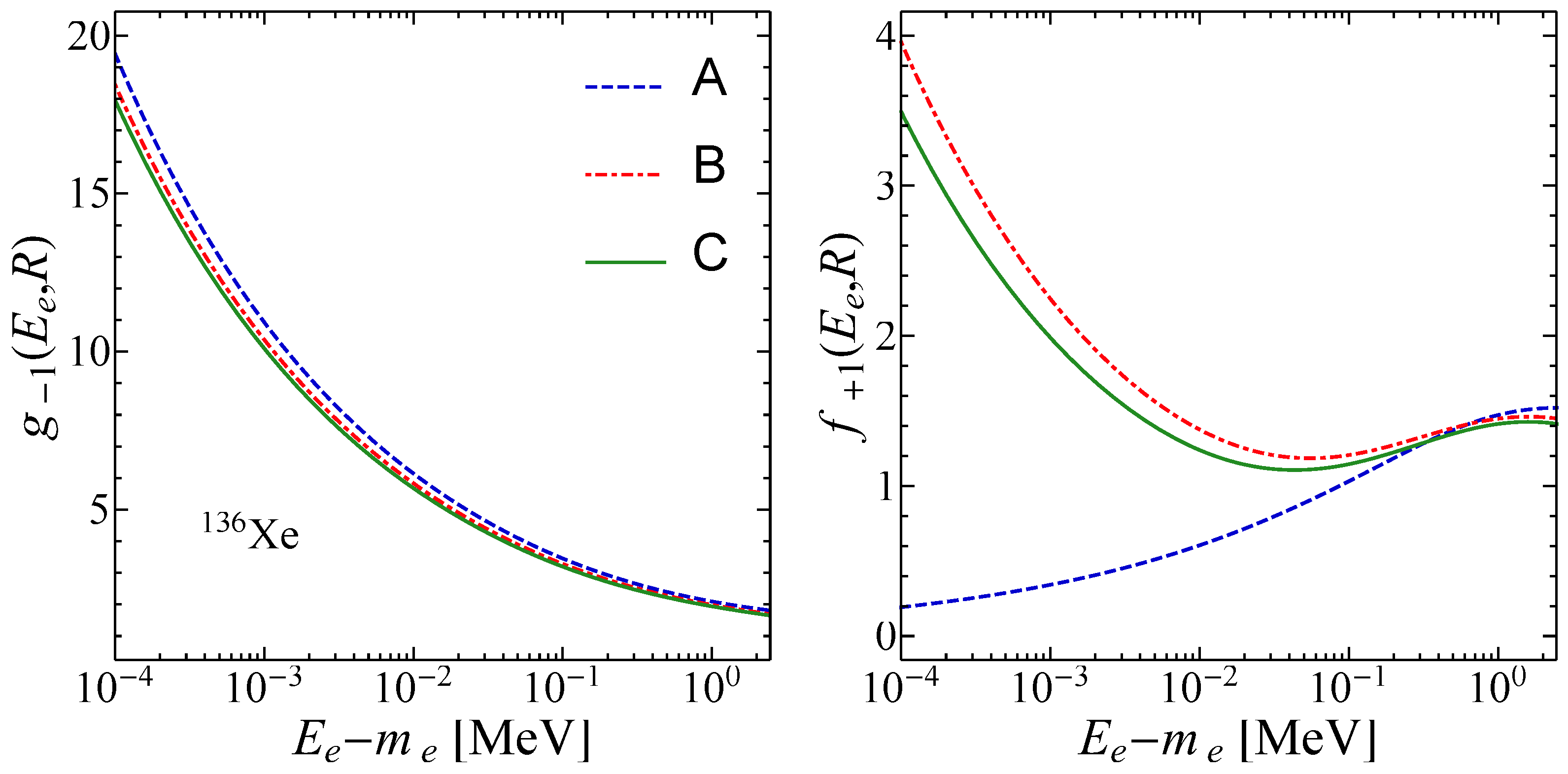
In Figure 1, we present the radial wave functions of an electron in spherical wave state from the double- emitter Xe, as functions of kinetic energy and evaluated on the surface of the daughter nucleus. We observe that the approximation scheme A, corresponding to leading finite-size Coulomb, is in good agreement with the other two approaches for but fails badly for , especially at low energies of the electron. We note that approximation schemes B and C are in good agreement in the representation intervals as a final remark.
5. Results and Discussion
The integration over all leptons energies in the decay rate is essential when predicting the half-life and the angular correlation coefficient of the emitted electrons. We performed the integration over the energies of the electrons numerically, with a 15-points Gauss-Kronrod quadrature. The integration over neutrino energy is performed analytically in the Appendix A.
In Table 1, we present the phase-space factors entering in the decay rate, that is, Equation (18), calculated within approximation schemes A, B, and C, for decay of Mo, Xe and Nd. As was already pointed out in [6], the phase-space factors calculated with exact relativistic electron wave functions (scheme C) are smaller than those provided by approximation scheme A. We can see that the results for obtained with scheme B are between the results obtained with schemes A and C. In the angular phase-space factors , we observe a good agreement between schemes A and B, and again smaller results from scheme C. The different behavior of and , for the same approximations schemes for the electronic wave functions, indicates that the angular correlation is sensitive to the treatment of the Coulomb interaction for the emitted electrons.
In Table 2, we update the values of the phase-space factors with the approximation scheme C for 11 nuclei of experimental interest. We took the Q-value for each nucleus from the experiment with the smallest uncertainty when available or from tables of recommended values [36], as it is the case of -decay of Sn. In what follows, we used just those values for the maximum sum of the electrons’ kinetic energies.
Considering , 0, , and , we present in Table 3 the values of the angular correlation coefficient , defined in Equation (26), for multiple nuclei of interest. For each nucleus, we display the fixed by the SSD relation and the energy difference between the lowest state of the intermediate nucleus and the ground state of the initial nucleus (see Equation (27)). Columns 5 and 6 in Table 3 represent the angular correlation coefficient results using the electronic wave function in approximation schemes A and C, respectively. Besides the fact that we obtain smaller results with scheme C compared with scheme A, we can also observe that the dependence of on is not linear.
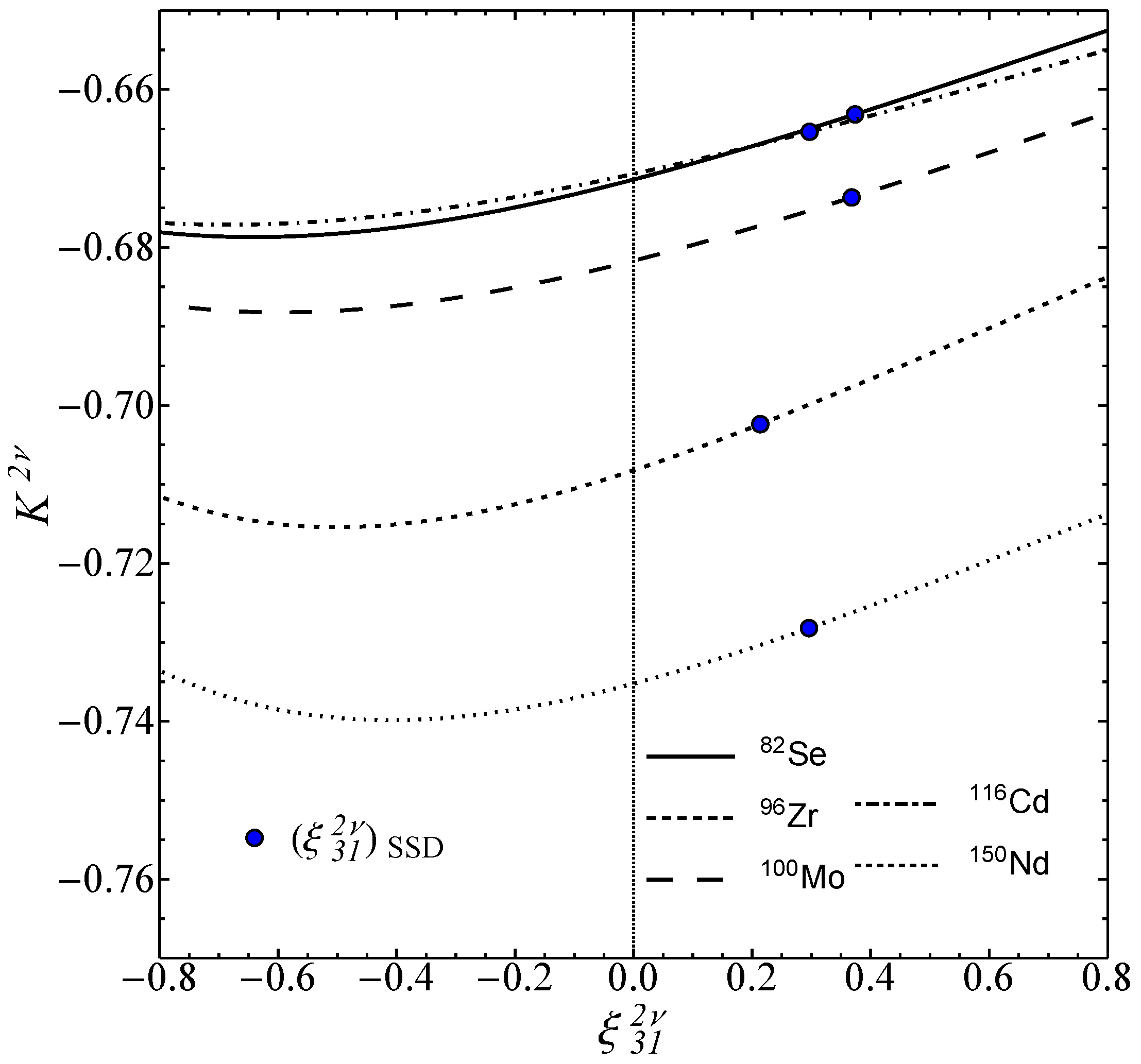
To emphasize the dependence on the ratio of the nuclear matrix elements we depict, in Figure 2, the angular correlation coefficient as a function of . The representation is done from to for all nuclei. We can see that is a quadratic function of for all nuclei, at least in the representation interval. If we assume the SSD in the process, then the unknown parameter is fixed to the value. We present with filled blue circles, in Figure 2, the values of the angular correlation coefficient evaluated at .
The integration over all leptons energies is crucial in calculating the global observables. Still, the integrand itself provides valuable information about the energy and angular distributions of the emitted electrons. The analytical approach for the integration over the neutrino energy (see Appendix A) ensures that we can evaluate the obtained distributions at any energetical point, not only in the points fixed by the numerical method of integration.
From the analytical expressions of the partial double distributions in Equation (A8), we can see that they exhibit a completely different behavior as functions of the electron energies, and . This fact is highlighted in Figure 3, where we present, for -decay of Mo, the contour plots of the partial double electron distribution normalized to the corresponding partial decay rate. The normalization procedure ensures that the normalized partial distributions do not depend on the ratios of nuclear matrix elements and .
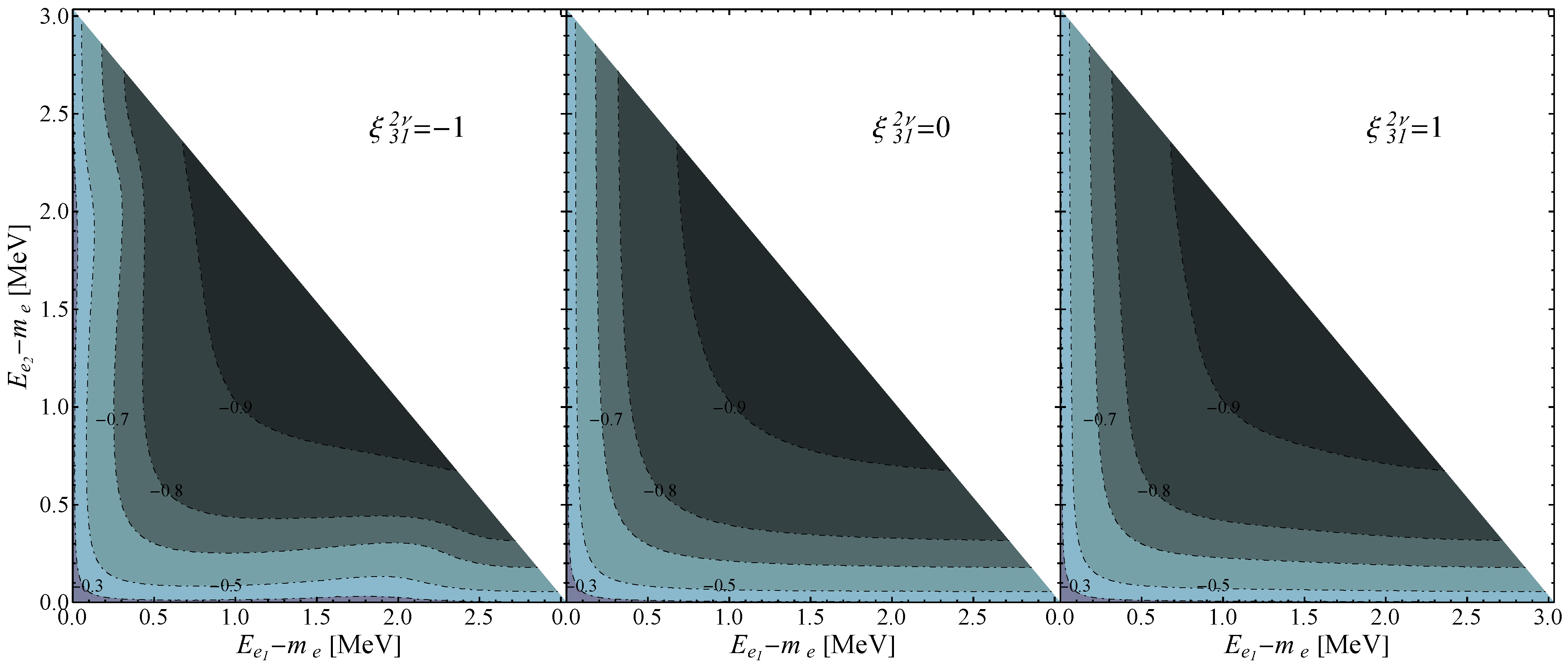
The angular correlation distribution as a function of the energies of the electrons and the ratios of the nuclear matrix elements can be found in Equation (A10). In Figure 4, we show, for Mo, the contour plots of the angular distributions for different values of as functions of the electron energies. The left, middle and right panels are obtained for , 0 and 1, respectively. The middle panel corresponds to the standard approximation angular distribution.
We compared the improved formalism presented in this paper with the exact SSD formalism of the -decay [21,22]. If we assume the SSD, the ratios and are fixed. We present the single electron differential decay rates normalized to the full width, in Figure 5, for Se, Mo and Nd. With a solid black line, we present the normalized single electron spectra within the exact SSD formalism [21,22], and with the blue dashed line, the spectra presented in Equation (A11). The value of the ratio fixed in SSD assumption can be found in the plots’ legend. In the lower panels, the residuals between exact and improved formalisms are plotted. We can conclude that the spectra are in a good agreement. A small disagreement appears only for low electron energy, which is not accessible by the double-beta experiments due to large background events.
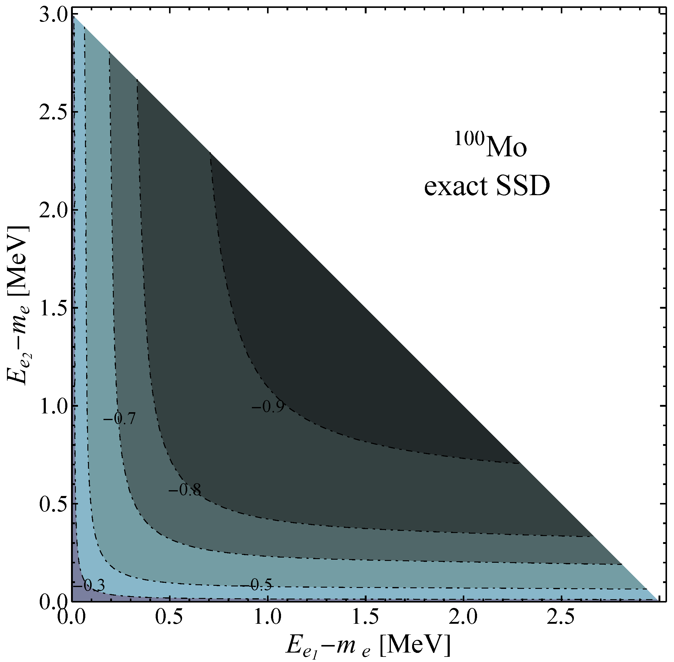
To compare the angular correlation distribution between the exact SSD formalism and the improved one, we display in Figure 6, the distribution reproduced within the exact SSD formalism. It should be noted that there are no significant deviations of this distribution from the one with positive from Figure 4. Considering the comparison of the single electron spectra and angular distributions, we can conclude that the improved formalism presented in this paper, with fixed by SSD assumption, is in excellent agreement with the exact SSD formalism.
6. Towards to Detection of Effective Axial-Vector Coupling
It was already pointed out in [6] that the calculation of can be more reliable than that of , because is saturated by contributions through the lightest states of the intermediate nucleus. The -decay half-life can be expressed with , and as follows:
that is, without explicit dependence on nuclear structure factor . The nuclear structure parameter can be deduced from the energy distribution of the emitted electrons or from the angular correlation factor as solution
of a quadratic equation with coefficients A, B and C, which are functions of the measured angular correlation factor:
The fact that for a measured angular correlation coefficient there are two possible values of , it can also be seen graphically from Figure 2. To determine the physical solution, a cross-check with the determination of from the energy distribution is necessary.
Suppose is reliably calculated, and is precisely obtained from the angular and energetic measurements. In that case, we can determine from the measured -decay half-life expression via Equation (47). A disagreement between deduced from the energy and angular distributions might indicate a new physics scenario observed in the data analysis of the -decay.
7. Summary and Conclusions
The -decay has been a subject of theoretical and experimental research for more than 85 years and remains an important topic in modern nuclear and particle physics. In the presented paper, the theoretical description of the angular distribution of outgoing electrons is achieved by considering the effect of lepton energies in energy denominators of the nuclear matrix elements via the Taylor expansion. It is claimed that by a precise measurement of angular correlation factor of the emitted electrons, the nuclear structure parameter can be fixed, which might allow determining the effective axial-vector coupling constant from the measured -decay half-life, once the nuclear matrix element is calculated reliably. A non-zero is a signature of the dominance of the Gamow-Teller over Fermi transitions in the -decay. A more accurate treatment of the nuclear physics aspects of the -decay will allow more reliability to address possible new physics scenarios associated with neutrino properties and interactions.
In the case of Mo and Nd, the NEMO-3 experiment already recorded a large number of -events describing all kinds of differential characteristics of emitted electrons. It would be difficult to reanalyze the recorded data within the improved formalism of this paper. However, many running and planed double beta decay experiments, for example, GERDA, CUORE, KamLAND-Zen, EXO, CUPID, LEGEND, and so forth, will achieve sufficiently large statistics to fix nuclear structure parameter from the energy distribution of emitted electrons. The potential of the SuperNEMO experiment, in which the first module Demonstrator is in a construction phase, will be able to measure this quantity even from the angular distribution. The angular information might also be obtained with high-pressure gaseous time-projection technology and pixelated detectors; however, the present methods have significant limitations. It goes without saying that there is continuous progress in double beta decay technologies, the ultimate goal of which is to register emitted electrons with high energy and angular resolutions.
Author Contributions
Conceptualization, F.Š.; methodology, O.N., R.D. and F.Š.; software, O.N.; validation, O.N., R.D., S.S. and F.Š.; formal analysis, O.N. and F.Š.; investigation, O.N.; resources, R.D., S.S. and F.Š.; data curation, O.N. and F.Š.; writing—original draft preparation, O.N. and F.Š.; writing—review and editing, O.N., R.D., S.S. and F.Š.; visualization, O.N. and F.Š.; supervision, F.Š.; project administration, F.Š.; funding acquisition, S.S. and F.Š. All authors have read and agreed to the published version of the manuscript.
Funding
F.Š. acknowledges support by the VEGA Grant Agency of the Slovak Republic under Contract No. 1/0607/20 and by the Ministry of Education, Youth and Sports of the Czech Republic under the INAFYM Grant No. CZ.02.1.01/0.0/0.0/16_019/0000766. S.S. acknowledges support by a grant of the Romanian Ministry of Research, Innovation and Digitization, CNCS-UEFISCDI, project number 99/2021, within PN-III-P4-ID-PCE-2020.
Institutional Review Board Statement
Not applicable.
Acknowledgments
The figures for this article have been created using the SciDraw scientific figure preparation system [47].
Conflicts of Interest
The authors declare no conflict of interest.
Appendix A. Integration over Neutrino Energy
Motivated to obtain an analytical expression for the angular correlation distribution , we performed the integration over the neutrino energy analytically. In what follows, we denote the integrals with,
where , functions are defined in Equation (19) and .
We used the following standard integrals,
and
The results can be expressed in the following compact form
where
We can write the normalized full double electron distribution as functions of the electron energies, and , and of the nuclear matrix elements ratios, and as
where
We can also define the partial double distributions normalized to the corresponding partial decay rate as
with .
To write the angular distribution in a compact form, we define also the dimensionless quantities,
The angular correlation distribution can be written as
The integration over one electron energy of the full double electron distribution, that is, Equation (A6), leads us to the single electron differential rate
References
- Goeppert-Mayer, M. Double Beta-Disintegration. Phys. Rev. 1935, 48, 512. [Google Scholar] [CrossRef]
- Elliott, S.R.; Hahn, A.A.; Moe, M.K. Direct Evidence for Two Neutrino Double Beta Decay in 82Se. Phys. Rev. Lett. 1987, 59, 2020. [Google Scholar] [CrossRef] [PubMed]
- Barabash, A. Precise Half-Life Values for Two-Neutrino Double-β Decay: 2020 Review. Universe 2020, 6, 159. [Google Scholar] [CrossRef]
- Štefánik, D.; Šimkovic, F.; Faessler, A. Structure of the two-neutrino double-β decay matrix elements within perturbation theory. Phys. Rev. C 2015, 91, 064311. [Google Scholar] [CrossRef]
- Šimkovic, F.; Smetana, A.; Vogel, P. 0νββ nuclear matrix elements, neutrino potentials and SU(4) symmetry. Phys. Rev. C 2018, 98, 064325. [Google Scholar] [CrossRef] [Green Version]
- Šimkovic, F.; Dvornický, R.; Štefánik, D.; Faessler, A. Improved description of the 2νββ-decay and a possibility to determine the effective axial-vector coupling constant. Phys. Rev. C 2018, 97, 034315. [Google Scholar] [CrossRef] [Green Version]
- Zen Collaboration. Precision measurement of the 136Xe two-neutrino ββ spectrum in KamLAND-Zen and its impact on the quenching of nuclear matrix elements. Phys. Rev. Lett. 2019, 122, 192501. [Google Scholar] [CrossRef] [PubMed] [Green Version]
- Suhonen, J.T. Value of the Axial-Vector Coupling Strength in β and ββ Decays: A Review. Front. Phys. 2017, 5, 55. [Google Scholar] [CrossRef]
- Suhonen, T.; Kostensalo, J. Double β Decay and the Axial Strength. Front. Phys. 2019, 7, 29. [Google Scholar] [CrossRef]
- Deppisch, F.F.; Gráf, L.; Šimkovic, F. Searching for New physics in two-neutrino double beta decay. Phys. Rev. Lett. 2020, 125, 171801. [Google Scholar] [CrossRef] [PubMed]
- Deppisch, F.F.; Gráf, L.; Rodejohann, W.; Xu, X.-J. Neutrino self-interactions and double beta decay. Phys. Rev. D 2020, 102, 051701. [Google Scholar] [CrossRef]
- Bolton, P.; Deppisch, F.F.; Gráf, L.; Šimkovic, F. Two-Neutrino Double Beta Decay with Sterile Neutrinos. Phys. Rev. D 2021, 103, 055019. [Google Scholar] [CrossRef]
- Barabash, A.S.; Dolgov, A.D.; Dvornický, R.; Šimkovic, F.; Smirnov, A.Y. Statistics of neutrinos and the double beta decay. Nucl. Phys. B 2007, 783, 90. [Google Scholar] [CrossRef] [Green Version]
- Albert, J.B.; Barbeau, P.S.; Beck, D.; Belov, V.; Breidenbach, M.; Brunner, T.; Burenkov, A.; Cao, G.F.; Chambers, C.; Cleveland, B.; et al. First search for Lorentz and CPT violation in double beta decay with EXO-200. Phys. Rev. D 2016, 93, 072001. [Google Scholar] [CrossRef] [Green Version]
- Azzolini, O.; Beeman, J.W.; Bellini, F.; Beretta, M.; Biassoni, M.; Brofferio, C.; Bucci, C.; Capelli, S.; Cardani, L.; Carniti, P.; et al. First search for Lorentz violation in double beta decay with scintillating calorimeters. Phys. Rev. D 2019, 100, 092002. [Google Scholar] [CrossRef]
- Niţescu, O.; Ghinescu, S.; Stoica, S. Lorentz violation effects in 2νββ decay. J. Phys. G Nucl. Part. Phys. 2020, 47, 055112. [Google Scholar] [CrossRef] [Green Version]
- Niţescu, O.; Ghinescu, S.; Mirea, M.; Stoica, S. Probing Lorentz violation in 2νββ using single electron spectra and angular correlations. Phys. Rev. D 2021, 103, L031701. [Google Scholar] [CrossRef]
- Arnold, R.; Augier, C.; Baker, J.; Barabash, A.S.; Brudanin, V.; Caffrey, A.J.; Caurier, E.; Egorov, V.; Errahmane, K.; Etienvre, A.I.; et al. Limits on different Majoron decay modes of 100Mo and 82Se for neutrinoless double beta decays in the NEMO-3 experiment. Nucl. Phys. A 2006, 765, 483. [Google Scholar] [CrossRef] [Green Version]
- Arnold, R.; Augier, C.; Barabash, A.S.; Basharina-Freshville, A.; Blondel, S.; Blot, S.; Bongrand, M.; Boursette, D.; Brudanin, V.; Busto, J.; et al. Detailed studies of 100Mo two-neutrino double beta decay in NEMO-3. Eur. Phys. J. C 2019, 79, 440. [Google Scholar] [CrossRef]
- Arnold, R.; Augier, C.; Barabash, A.S.; Basharina-Freshville, A.; Blondel, S.; Blot, S.; Bongrand, M.; Boursette, D.; Brudanin, V.; Busto, J.; et al. Search for neutrinoless quadruple-β decay of 150Nd with the NEMO-3 detector. Phys. Rev. Lett. 2017, 119, 041801. [Google Scholar] [CrossRef] [PubMed] [Green Version]
- Šimkovic, F.; Domin, P.; Semenov, S.V. The single state dominance hypothesis and the two-neutrino double beta decay of 100Mo. J. Phys. G 2001, 27, 2233. [Google Scholar] [CrossRef] [Green Version]
- Domin, P.; Kovalenko, S.; Šimkovic, F.; Semenov, S.V. Neutrino accompanied β±β±, β+/EC and EC/EC processes within single state dominance hypothesis. Nucl. Phys. A 2005, 753, 337. [Google Scholar] [CrossRef] [Green Version]
- Civitarese, O.; Suhonen, J. Contributions of unique first-forbidden transitions to two-neutrino double-β-decay half-lives. Nuclear Phys. A 1996, 607, 152–162. [Google Scholar] [CrossRef]
- Zyla, P.A.; Barnett, R.M.; Beringer, J.; Dahl, O.; Dwyer, D.A.; Groom, D.E.; Lin, C.J.; Lugovsky, K.S.; Pianori, E.; Robinson, D.J.; et al. (Particle Data Group), Review of Particle Physics. Prog. Theor. Exp. Phys. 2020, 2020, 083C01. [Google Scholar]
- Abad, J.; Morales, A.; Nunez-Lagos, R.; Pacheco, A. An estimation of the rates of (two-neutrino) double beta decay and related processes. Ann. Fis. A 1984, 80, 9. [Google Scholar] [CrossRef]
- Azzolini, O.; Beeman, J.W.; Bellini, F.; Beretta, M.; Biassoni, M.; Brofferio, C.; Bucci, C.; Capelli, S.; Cardani, L.; Carniti, P.; et al. Evidence of Single State Dominance in the Two-Neutrino Double-β Decay of 82Se with CUPID-0. Phys. Rev. Lett. 2019, 123, 262501. [Google Scholar] [CrossRef] [PubMed] [Green Version]
- Rose, M.E. Relativistic Electron Theory; John Wiley and Sons: Hoboken, NJ, USA, 1961. [Google Scholar]
- Doi, M.; Kotani, T.; Takasugi, E. Double Beta Decay and Majorana Neutrino. Prog. Theor. Suppl. 1985, 83, 1. [Google Scholar] [CrossRef] [Green Version]
- Beresteckij, V.B.; Lifshitz, E.M.; Pitaevskij, L.P. Quantum Electrodynamics; Nauka: Moscow, Russia, 1989; Volume IV. [Google Scholar]
- Esposito, S. Majorana solution of the Thomas–Fermi equation. Am. J. Phys. 2002, 70, 852. [Google Scholar] [CrossRef] [Green Version]
- Kotila, J.; Iachello, F. Phase-space factors for double-β decay. Phys. Rev. C 2012, 85, 034316. [Google Scholar] [CrossRef] [Green Version]
- Stoica, S.; Mirea, M. New calculations for phase space factors involved in double-β decay. Phys. Rev. C 2013, 88, 037303. [Google Scholar] [CrossRef] [Green Version]
- Mirea, M.; Pahomi, T.; Stoica, S. Values of the phase space factors involved in double beta decay. Rom. Rep. Phys. 2015, 67, 872–889. [Google Scholar]
- Salvat, F.; Fernandez-Varea, J.M.; Williamson, W., Jr. Accurate numerical solution of the radial Schrödinger and Dirac wave equations. Comput. Phys. Commun. 1995, 90, 151. [Google Scholar] [CrossRef]
- Salvat, F.; Mayol, R. Accurate numerical solution of the Schrödinger and Dirac wave equations for central fields. Comput. Phys. Commun. 1991, 62, 65. [Google Scholar] [CrossRef]
- Wang, M.; Huang, W.J.; Kondev, F.G.; Audi, G.; Naimi, S. The AME 2020 atomic mass evaluation (II). Tables, graphs and references. Chin. Phys. C 2021, 45, 030003. [Google Scholar] [CrossRef]
- Bustabad, S.; Bollen, G.; Brodeur, M.; Lincoln, D.L.; Novario, S.J.; Redshaw, M.; Ringle, R.; Schwarz, S.; Valverde, A.A. First direct determination of the 48Ca double-β decay Q value. Phys. Rev. C 2013, 88, 022501. [Google Scholar] [CrossRef] [Green Version]
- Mount, B.J.; Redshaw, M.; Myers, E.G. Double-β-decay Q values of 74Se and 76Ge. Phys. Rev. C 2010, 81, 032501. [Google Scholar] [CrossRef]
- Lincoln, D.L.; Holt, J.D.; Bollen, G.; Brodeur, M.; Bustabad, S.; Engel, J.; Novario, S.J.; Redshaw, M.; Ringle, R.; Schwarz, S. First Direct Double-β Decay Q-Value Measurement of 82Se in Support of Understanding the Nature of the Neutrino. Phys. Rev. Lett. 2013, 110, 012501. [Google Scholar] [CrossRef] [PubMed] [Green Version]
- Alanssari, M.; Frekers, D.; Eronen, T.; Canete, L.; Dilling, J.; Haaranen, M.; Hakala, J.; Holl, M.; Ješkovský, M.; Jokinen, A.; et al. Single and Double Beta-Decay Q Values among the Triplet 96Zr, 96Nb, and 96Mo. Phys. Rev. Lett. 2016, 116, 072501. [Google Scholar] [CrossRef] [PubMed] [Green Version]
- Rahaman, S.; Elomaa, V.V.; Eronen, T.; Hakala, J.; Jokinen, A.; Julin, J.; Kankainen, A.; Saastamoinen, A.; Suhonen, J.; Weber, C.; et al. Q values of the 76Ge and 100Mo double-beta decays. Phys. Lett. B 2008, 662, 111. [Google Scholar] [CrossRef] [Green Version]
- Fink, D.; Barea, J.; Beck, D.; Blaum, K.; Böhm, C.; Borgmann, C.; Breitenfeldt, M.; Herfurth, F.; Herlert, A.; Kotila, J.; et al. Q Value and Half-Lives for the Double-β-Decay Nuclide 110Pd. Phys. Rev. Lett. 2012, 108, 062502. [Google Scholar] [CrossRef] [PubMed] [Green Version]
- Rahaman, S.; Elomaa, V.-V.; Eronen, T.; Hakala, J.; Jokinen, A.; Kankainen, A.; Rissanen, J.; Suhonen, J.; Weber, C.; Äystö, J. Double-beta decay Q values of 116Cd and 130Te. Phys. Lett. B 2011, 703, 412. [Google Scholar] [CrossRef] [Green Version]
- Redshaw, M.; Mount, B.J.; Myers, E.G.; Avignone, F.T. Masses of 130Te and 130Xe and Double-β-Decay Q Value of 130Te. Phys. Rev. Lett. 2009, 102, 212502. [Google Scholar] [CrossRef] [PubMed] [Green Version]
- Redshaw, M.; Wingfield, E.; McDaniel, J.; Myers, E.G. Mass and Double-Beta-Decay Q Value of 136Xe. Phys. Rev. Lett. 2007, 98, 053003. [Google Scholar] [CrossRef] [PubMed]
- Kolhinen, V.S.; Eronen, T.; Gorelov, D.; Hakala, J.; Jokinen, A.; Kankainen, A.; Moore, I.D.; Rissanen, J.; Saastamoinen, A.; Suhonen, J.; et al. Double-β decay Q value of 150Nd. Phys. Rev. C 2010, 82, 022501. [Google Scholar] [CrossRef]
- Caprio, M. LevelScheme: A level scheme drawing and scientific figure preparation system for Mathematica. Comput. Phys. Commun. 2005, 171, 107. [Google Scholar] [CrossRef] [Green Version]
Figure 1.
Electron radial wave functions in spherical wave state for an electron emitted in the double- decay of Xe, as functions of the kinetic energy evaluated on the surface of the final nucleus fm.
Figure 1.
Electron radial wave functions in spherical wave state for an electron emitted in the double- decay of Xe, as functions of the kinetic energy evaluated on the surface of the final nucleus fm.

Figure 2.
The angular correlation coefficient between the electrons emitted in decay of Se, Zr, Mo, Cd, and Nd, as functions of . The filled blue circles indicate the values of for the ratio of the nuclear matrix elements fixed by the SSD assumption, . In the case of Se and Cd, the right filled circle correspond to Se and the left one to Cd. We used the approximation scheme C for the relativistic wave function of the emitted electrons.

Figure 3.
Normalized to unity partial double energy distributions , as functions of the kinetic energies of the electrons, for (top left), (bottom left), (top right) and (bottom right). All distributions are in units of MeV for electrons emitted in double decay of Mo. The distributions are obtained using the screened exact finite-size Coulomb wave functions for electron state.
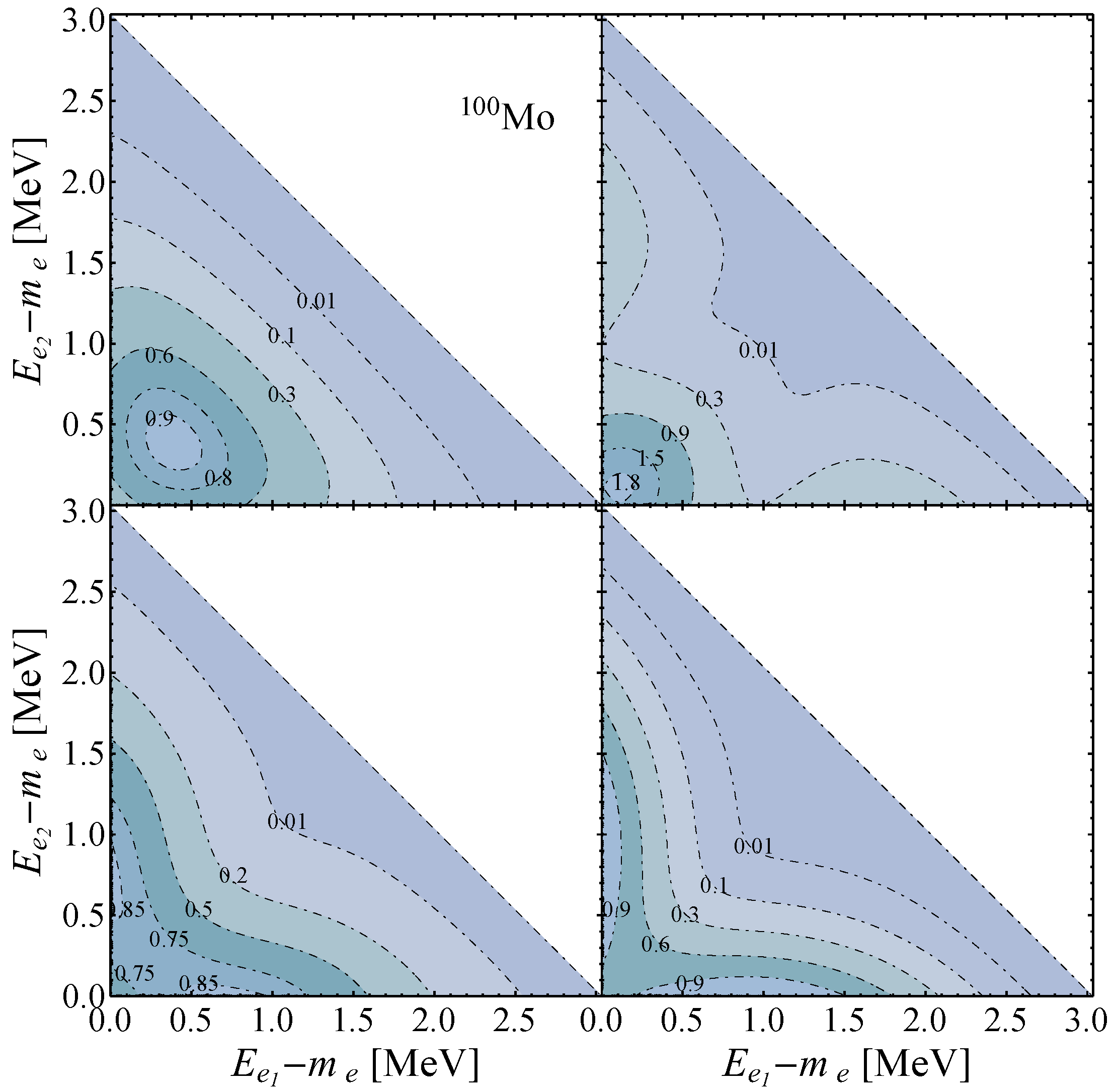
Figure 4.
The angular correlation as function of electron energies emitted in the -decay of Mo. The distributions are obtained using , 0 and 1. The distributions were calculated by using the screened exact finite-size Coulomb wave functions for electron state.
Figure 4.
The angular correlation as function of electron energies emitted in the -decay of Mo. The distributions are obtained using , 0 and 1. The distributions were calculated by using the screened exact finite-size Coulomb wave functions for electron state.

Figure 5.
Normalized single electron spectra for Se, Mo and Nd assuming the single state dominance. We compare the exact SSD [21,22] with the Taylor expansion with ratio of the nuclear matrix elements fixed by SSD.
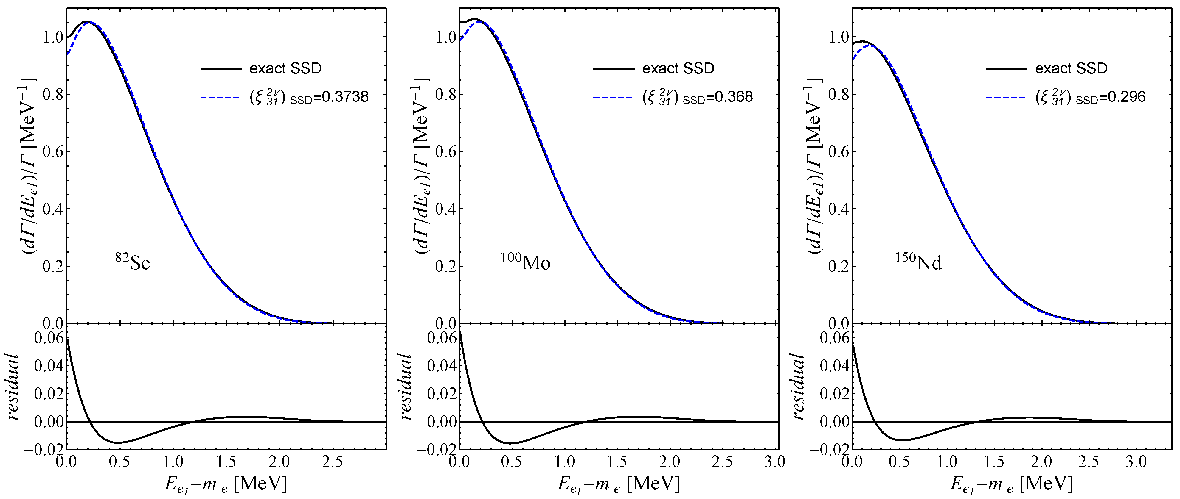
Figure 6.
The angular correlation as function of energies of electrons emitted in -decay of Mo. The distribution is obtained using the exact SSD formalism presented in [21,22] and the screened exact finite-size Coulomb wave functions for electron state.

Table 1.
Phase space factors and with for decay of Mo, Xe and Nd. The results are obtained using different approximations for the radial wave functions and of the electron: (A) The standard approximation of Doi et al. [28]. (B) The analytical solution of the Dirac equation for a point-like nucleus [29]. (C) The exact solution of the Dirac equation for a uniform charge distribution of the nucleus screened by the atomic electronic cloud. The results are presented in . For each nucleus and each phase space factor we present the percent deviation between approximation schemes A and B, , and the percent deviation between approximation schemes A and C, , with or .
| Nucleus | Elec. w. f. | ||||
| Mo | A | ||||
| B | |||||
| C | |||||
| Xe | A | ||||
| B | |||||
| C | |||||
| Nd | A | ||||
| B | |||||
| C | |||||
| Nucleus | Elec. w. f. | ||||
| Mo | A | ||||
| B | |||||
| C | |||||
| Xe | A | ||||
| B | |||||
| C | |||||
| Nd | A | ||||
| B | |||||
| C | |||||
Table 2.
Phase space factors and with , in , obtained using the screened exact finite-size Coulomb wave functions for electron state. The Q values are taken from the experiments with the smallest uncertainty when available, or from tables of recommended value [36].
Table 2.
Phase space factors and with , in , obtained using the screened exact finite-size Coulomb wave functions for electron state. The Q values are taken from the experiments with the smallest uncertainty when available, or from tables of recommended value [36].
| Nucleus | Q [MeV] | ||||
| Ca | [37] | ||||
| Ge | [38] | ||||
| Se | [39] | ||||
| Zr | [40] | ||||
| Mo | [41] | ||||
| Pd | [42] | ||||
| Cd | [43] | ||||
| Sn | [36] | ||||
| Te | [44] | ||||
| Xe | [45] | ||||
| Nd | [46] | ||||
| Nucleus | [MeV] | ||||
| Ca | [37] | ||||
| Ge | [38] | ||||
| Se | [39] | ||||
| Zr | [40] | ||||
| Mo | [41] | ||||
| Pd | [42] | ||||
| Cd | [43] | ||||
| Sn | [36] | ||||
| Te | [44] | ||||
| Xe | [45] | ||||
| Nd | [46] |
Table 3.
The values of the angular correlation coefficient for different values of . We assume the approximation scheme A and C for the relativistic wave function of the emitted electrons. For each nuclei, we display the energy difference in MeV, necessary to calculate via Equation (27).
Table 3.
The values of the angular correlation coefficient for different values of . We assume the approximation scheme A and C for the relativistic wave function of the emitted electrons. For each nuclei, we display the energy difference in MeV, necessary to calculate via Equation (27).
| A | C | ||||
|---|---|---|---|---|---|
| Nucleus | |||||
| Se | −0.338 | 0.139 | −0.2 | −0.649 | −0.675 |
| 0.0 | −0.645 | −0.671 | |||
| 0.2 | −0.641 | −0.667 | |||
| 0.4 | −0.636 | −0.662 | |||
| 0.6 | −0.630 | −0.657 | |||
| Zr | 0.021 | 0.046 | −0.2 | −0.681 | −0.713 |
| 0.0 | −0.676 | −0.708 | |||
| 0.2 | −0.669 | −0.703 | |||
| 0.4 | −0.663 | −0.697 | |||
| 0.6 | −0.656 | −0.690 | |||
| Mo | −0.343 | 0.135 | −0.2 | −0.646 | −0.685 |
| 0.0 | −0.642 | −0.682 | |||
| 0.2 | −0.637 | −0.677 | |||
| 0.4 | −0.632 | −0.673 | |||
| 0.6 | −0.627 | −0.668 | |||
| Cd | −0.043 | 0.088 | −0.2 | −0.620 | −0.674 |
| 0.0 | −0.616 | −0.671 | |||
| 0.2 | −0.612 | −0.667 | |||
| 0.4 | −0.607 | −0.663 | |||
| 0.6 | −0.603 | −0.659 | |||
| Nd | −0.315 | 0.087 | −0.2 | −0.666 | −0.738 |
| 0.0 | −0.661 | −0.735 | |||
| 0.2 | −0.655 | −0.731 | |||
| 0.4 | −0.648 | −0.725 | |||
| 0.6 | −0.641 | −0.719 |
Publisher’s Note: MDPI stays neutral with regard to jurisdictional claims in published maps and institutional affiliations. |
© 2021 by the authors. Licensee MDPI, Basel, Switzerland. This article is an open access article distributed under the terms and conditions of the Creative Commons Attribution (CC BY) license (https://creativecommons.org/licenses/by/4.0/).
Share and Cite
MDPI and ACS Style
Niţescu, O.; Dvornický, R.; Stoica, S.; Šimkovic, F. Angular Distributions of Emitted Electrons in the Two-Neutrino ββ Decay. Universe 2021, 7, 147. https://doi.org/10.3390/universe7050147
AMA Style
Niţescu O, Dvornický R, Stoica S, Šimkovic F. Angular Distributions of Emitted Electrons in the Two-Neutrino ββ Decay. Universe. 2021; 7(5):147. https://doi.org/10.3390/universe7050147
Chicago/Turabian StyleNiţescu, Ovidiu, Rastislav Dvornický, Sabin Stoica, and Fedor Šimkovic. 2021. "Angular Distributions of Emitted Electrons in the Two-Neutrino ββ Decay" Universe 7, no. 5: 147. https://doi.org/10.3390/universe7050147
Note that from the first issue of 2016, this journal uses article numbers instead of page numbers. See further details here.