
Dual Memory LSTM with Dual Attention Neural Network for Spatiotemporal Prediction

Abstract
:1. Introduction
2. Literature Review
3. DMA Neural Network
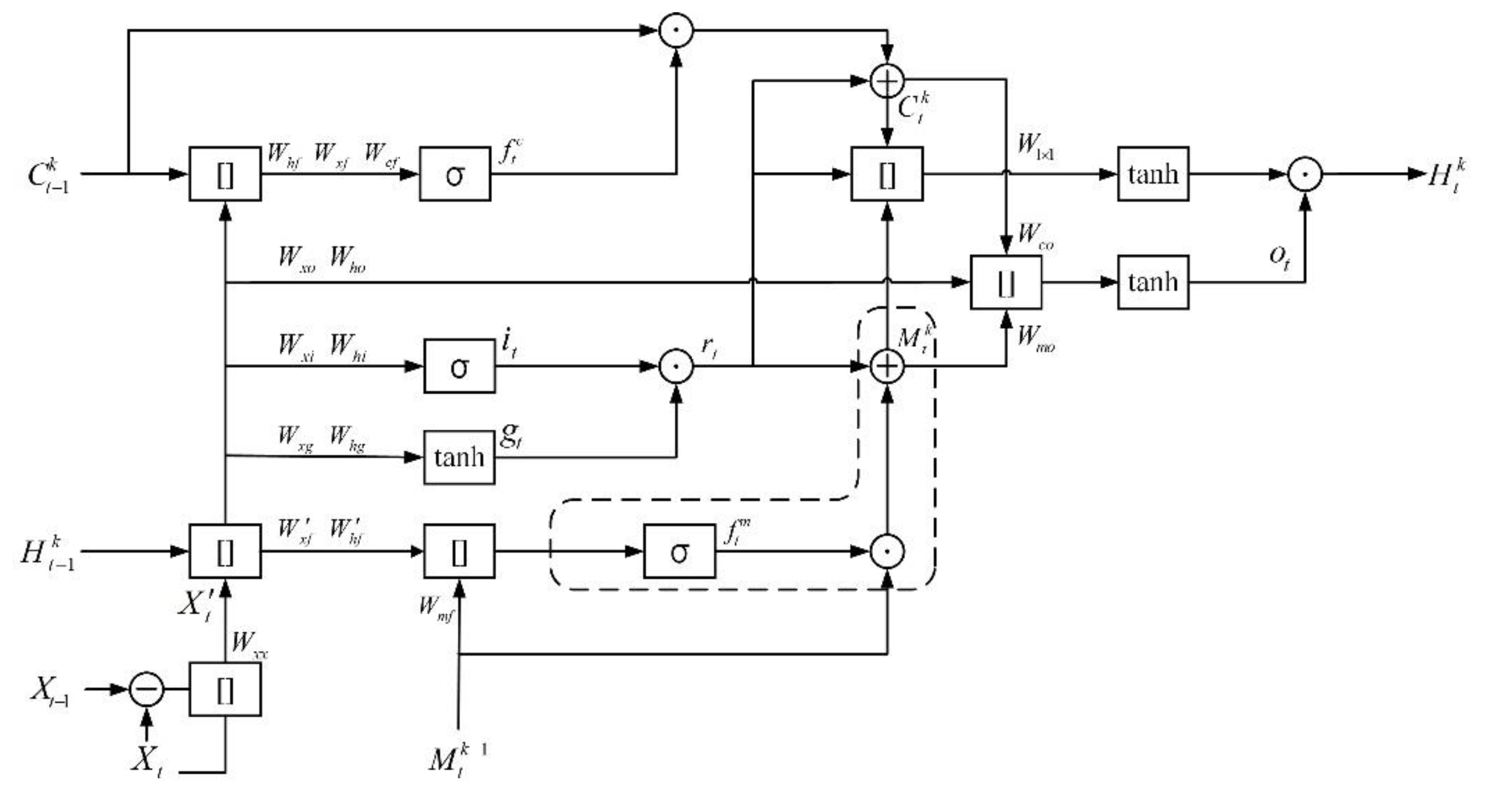
3.1. Dual Memory LSTM
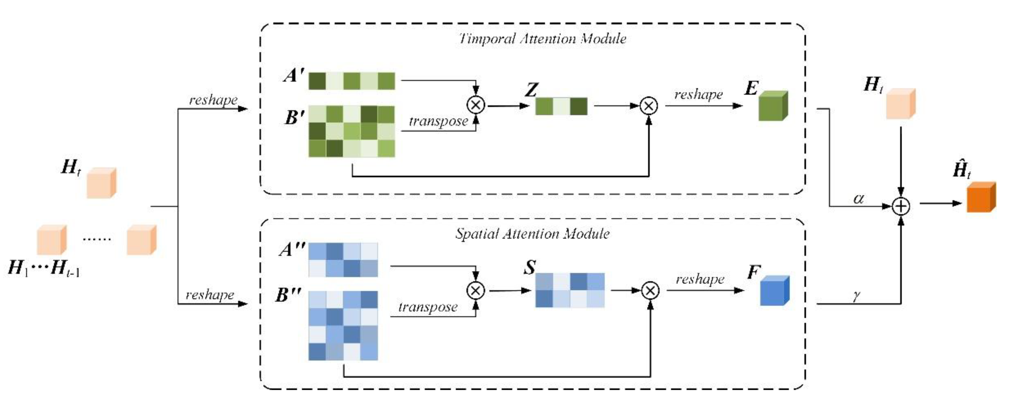
3.2. Dual Attention Mechanism
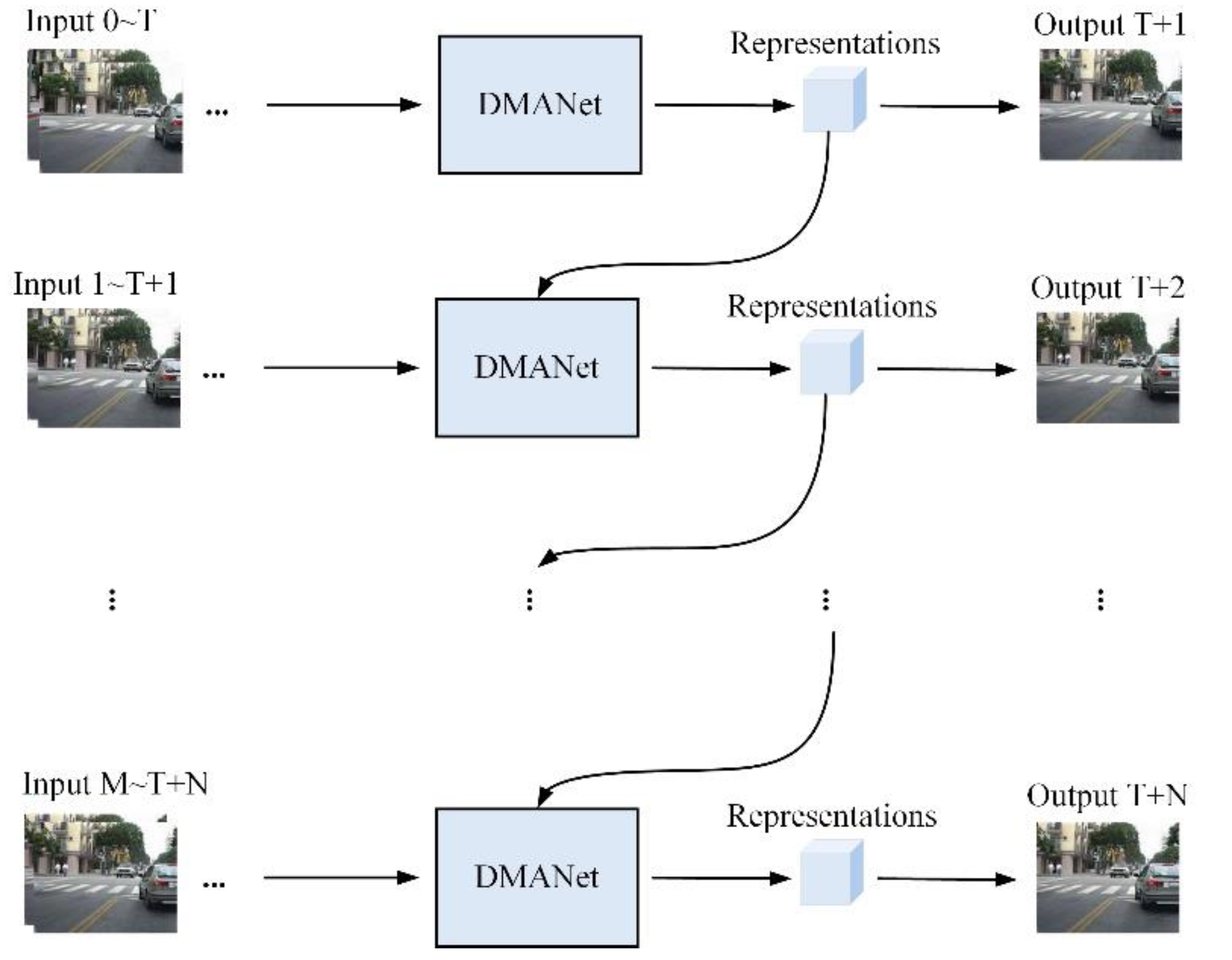
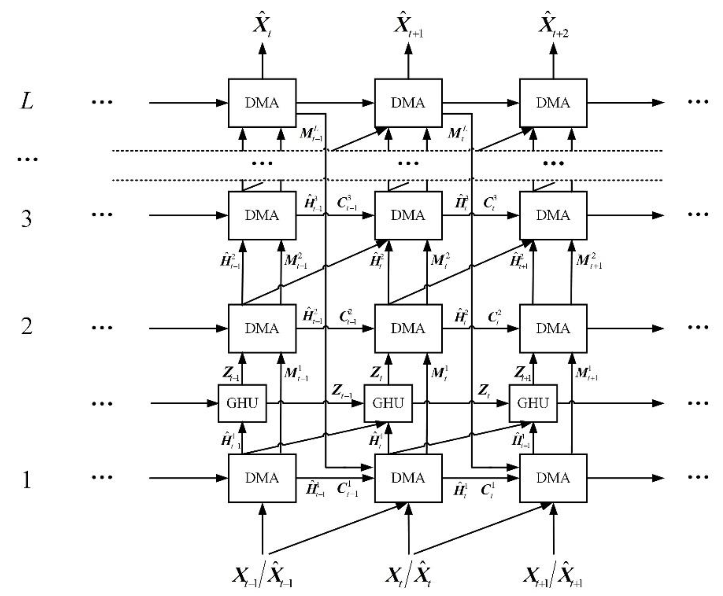
3.3. DMANet
3.4. Training Method
4. Experiments
4.1. Dataset and Implements
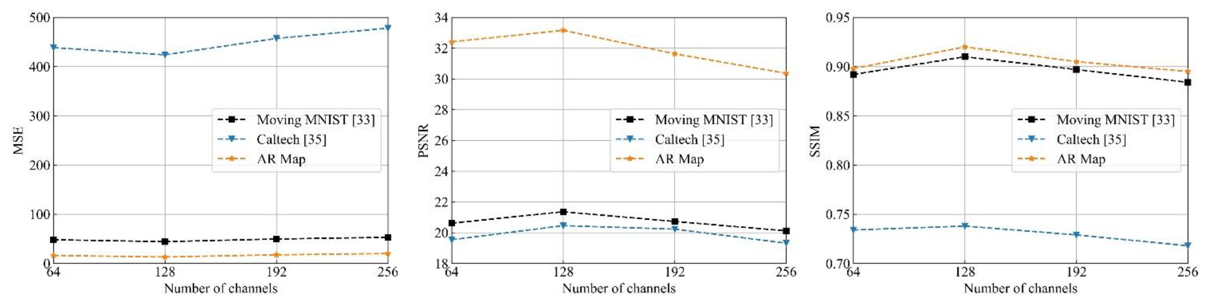
4.2. Parameter Analyses
4.3. DMLSTM Unit and the Dual Attention Mechanism Evaluation
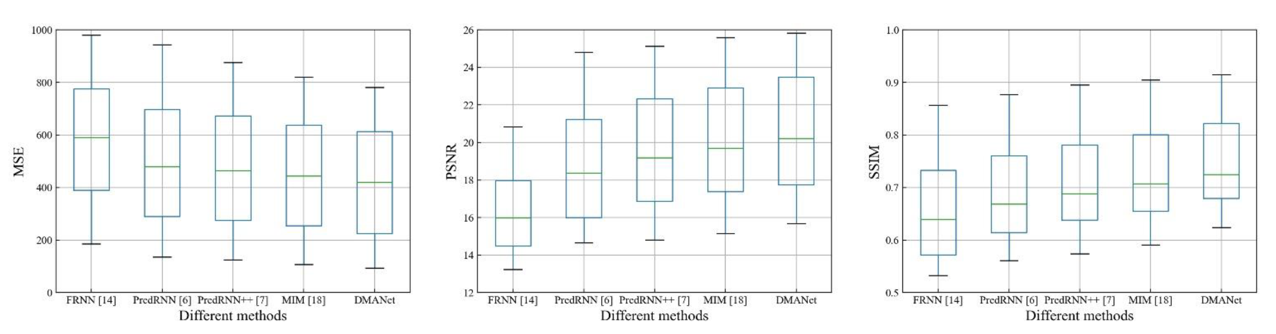
4.4. Comparisons with Some State-of-the-Art Methods
5. Conclusions
Author Contributions
Funding
Institutional Review Board Statement
Informed Consent Statement
Data Availability Statement
Conflicts of Interest
References
- Yao, Y.; Atkins, E.; Johnson-Roberson, M.; Vasudevan, R.; Du, X. Bitrap: Bi-directional pedestrian trajectory prediction with multi-modal goal estimation. IEEE Robot. Autom. Lett. 2021, 2, 1463–1470. [Google Scholar] [CrossRef]
- Song, Z.; Sui, H.; Li, H. A hierarchical object detection method in large-scale optical remote sensing satellite imagery using saliency detection and CNN. Int. J. Remote Sens. 2021, 42, 2827–2847. [Google Scholar] [CrossRef]
- Li, Y.; Cai, Y.; Li, J.; Lang, S.; Zhang, X. Spatio-temporal unity networking for video anomaly detection. IEEE Access 2019, 1, 172425–172432. [Google Scholar] [CrossRef]
- Yurtsever, E.; Lambert, J.; Carballo, A.; Takeda, K. A survey of autonomous driving: Common practices and emerging technologies. IEEE Access 2020, 8, 58443–58469. [Google Scholar] [CrossRef]
- Shi, X.; Chen, Z.; Wang, H.; Yeung, D.Y. Convolutional LSTM network: A machine learning approach for precipitation nowcasting. In Proceedings of the 29th Conference on Neural Information Processing Systems, Montreal, QC, Canada, 7–12 June 2015; pp. 802–810. [Google Scholar]
- Wang, Y.; Li, M.; Wang, J.; Gao, Z.; Yu, P. PredRNN: Recurrent neural networks for predictive learning using spatiotemporal LSTMs. In Proceedings of the 31st Conference on Neural Information Processing Systems, Long Beach, BC, Canada, 4–9 December 2017; pp. 879–888. [Google Scholar]
- Wang, Y.; Gao, Z.; Long, M.; Wang, J.; Yu, P. PredRNN++: Towards a resolution of the deep-in-time dilemma in spatiotemporal predictive learning. In Proceedings of the 35th International Conference on Machine Learning, Stockholm, Sweden, 10–15 April 2019; pp. 5123–5132. [Google Scholar]
- Goodfellow, I.J.; Pouget-Abadie, J.; Mirza, M.; Xu, B.; Warde-Farley, D. Generative adversarial networks. In Proceedings of the 28th Conference on Neural Information Processing Systems, Montreal, QC, Canada, 8–13 December 2014; pp. 2672–2680. [Google Scholar]
- Ivanovic, B.; Karen, L.; Edward, S.; Pavone, M. Multimodal deep generative models for trajectory prediction: A conditional variational autoencoder approach. IEEE Robot. Autom. Lett. 2021, 2, 295–302. [Google Scholar] [CrossRef]
- Rumelhart, D.; Hinton, G.; Williams, R. Learning representations by back-propagating errors. Nature 1986, 1, 533–536. [Google Scholar] [CrossRef]
- Hochreiter, S.; Schmidhuber, J. Long short-term memory. Neural Comput. 1997, 8, 1735–1780. [Google Scholar] [CrossRef]
- Sutskever, I.; Vinyals, O.; Le, Q. Sequence to sequence learning with neural networks. In Proceedings of the Advances in Neural Information Processing Systems, Montreal, QC, Canada, 8–13 December 2014; pp. 3104–3112. [Google Scholar]
- Das, M.; Ghosh, S. A deep-learning-based forecasting ensemble to predict missing data for remote sensing analysis. IEEE J. Sel. Top. Appl. Earth Observ. Remote Sens. 2017, 12, 5228–5236. [Google Scholar] [CrossRef]
- Oliu, M.; Selva, J.; Escalera, S. Folded recurrent neural networks for future video prediction. In Proceedings of the 15th European Conference on Computer Vision, Munich, Germany, 8–14 December 2018; pp. 716–731. [Google Scholar]
- Seng, D.; Zhang, Q.; Zhang, X.; Chen, G.; Chen, X. Spatiotemporal prediction of air quality based on LSTM neural network. Alex. Eng. J. 2021, 60, 2021–2032. [Google Scholar] [CrossRef]
- Abed, A.; Ramin, Q.; Abed, A. The automated prediction of solar flares from SDO images using deep learning. Adv. Space Res. 2021, 67, 2544–2557. [Google Scholar] [CrossRef]
- Li, S.; Fang, J.; Xu, H.; Xue, J. Video frame prediction by deep multi-branch mask network. IEEE Trans. Circuits Syst. Video Technol. 2020, 4, 1–12. [Google Scholar] [CrossRef]
- Wang, Y.; Zhang, J.; Zhu, H.; Long, M.; Wang, J.; Yu, P. Memory in memory: A predictive neural network for learning higher-order non-stationarity from spatiotemporal dynamics. In Proceedings of the IEEE Conference on Computer Vision and Pattern Recognition, Long Beach, BC, Canada, 16–20 June 2020; pp. 9146–9154. [Google Scholar]
- Chen, X.; Xu, C.; Yang, X.; Yang, X.; Tao, D. Long-term video prediction via criticization and retrospection. IEEE Trans. Image Process. 2020, 29, 7090–7103. [Google Scholar] [CrossRef]
- Neda, E.; Reza, F. AptaNet as a deep learning approach for aptamer-protein interaction prediction. Sci. Re. 2021, 11, 6074–6093. [Google Scholar]
- Shen, B.; Ge, Z. Weighted nonlinear dynamic system for deep extraction of nonlinear dynamic latent variables and industrial application. IEEE Trans. Ind. Inform. 2021, 5, 3090–3098. [Google Scholar] [CrossRef]
- Zhou, J.; Dai, H.; Wang, H.; Wang, T. Wide-attention and deep-composite model for traffic flow prediction in transportation cyber-physical systems. IEEE Trans. Ind. Inform. 2021, 17, 3431–3440. [Google Scholar] [CrossRef]
- Patil, K.; Deo, M. Basin-scale prediction of sea surface temperature with artificial neural Networks. J. Atmos. Ocean. Technol. 2018, 7, 1441–1455. [Google Scholar] [CrossRef]
- Amato, F.; Guinard, F.; Robert, S.; Kanevski, M. A novel framework for spatio-temporal prediction of environmental data using deep learning. Sci. Rep. 2020, 10, 22243–22254. [Google Scholar] [CrossRef]
- Yan, J.; Qin, G.; Zhao, R.; Liang, Y.; Xu, Q. Mixpred: Video prediction beyond optical flow. IEEE Access 2019, 1, 185654–185665. [Google Scholar] [CrossRef]
- Wang, Y.; Jiang, L.; Yang, M.; Li, L.; Long, M.; Li, F. Eidetic 3D LSTM: A model for video prediction and beyond. In Proceedings of the International Conference on Learning Representations, New Orleans, LA, USA, 6–9 May 2019; pp. 1–14. [Google Scholar]
- Vaswani, A.; Shazeer, N.; Parmar, N.; Uszkoreit, J.; Jones, L. Attention is all you need. In Proceedings of the 31st Conference on Neural Information Processing Systems, Long Beach, BC, Canada, 4–9 December 2017; pp. 5998–6008. [Google Scholar]
- Chen, Y.; Kalantidis, Y.; Li, J.; Feng, J. A2 nets: Double attention networks. In Proceedings of the 32nd Conference on Neural Information Processing Systems, Montreal, QC, Canada, 2–8 December 2018; pp. 352–361. [Google Scholar]
- Huang, Z.; Wang, X.; Wei, Y.; Huang, L.; Shi, H. Ccnet: Criss-cross attention for semantic segmentation. IEEE Trans. Pattern Anal. Mach. Intell. 2020, 1, 1–11. [Google Scholar] [CrossRef]
- Fu, J.; Liu, J.; Tian, H.; Li, Y. Dual attention network for scene segmentation. In Proceedings of the IEEE Conference on Computer Vision and Pattern Recognition, Long Beach, BC, Canada, 16–20 June 2019; pp. 3146–3154. [Google Scholar]
- Wang, Z.; Bovik, A.; Sheikh, H. Image quality assessment: From error visibility to structural similarity. IEEE Trans. Image Process. 2004, 4, 600–612. [Google Scholar] [CrossRef] [Green Version]
- Liu, Q.; Lu, S.; Lan, L. Yolov3 attention face detector with high accuracy and efficiency. Comp. Syst. Sci. Eng. 2021, 37, 283–295. [Google Scholar]
- Li, X.; Xu, F.; Xin, L. Dual attention deep fusion semantic segmentation networks of large-scale satellite remote-sensing images. Int. J. Remote Sens. 2021, 42, 3583–3610. [Google Scholar] [CrossRef]
- Srivastava, N.; Mansimov, E.; Salakhutdinov, R. Unsupervised learning of video representations using LSTMs. In Proceedings of the 32nd International Conference on Machine Learning, Lille, France, 6–11 June 2015; pp. 843–852. [Google Scholar]
- Geiger, A.; Lenz, P.; Stiller, C.; Urtasun, R. Vision meets robotics: The KITTI dataset. Int. J. Robot. Res. 2013, 32, 1231–1237. [Google Scholar] [CrossRef] [Green Version]
- Dollar, P.; Wojek, C.; Schiele, B.; Perona, P. Pedestrian detection: A benchmark. In Proceedings of the IEEE Conference on Computer Vision and Pattern Recognition, Miami, FL, USA, 20–25 June 2009; pp. 304–311. [Google Scholar]
- Liu, J.; Jin, B.; Yang, J.; Xu, L. Sea surface temperature prediction using a cubic B-spline interpolation and spatiotemporal attention mechanism. Remote Sens. Lett. 2021, 12, 12478–12487. [Google Scholar] [CrossRef]


| Acronym | Describe |
|---|---|
| DMANet | DMANet is Dual Memory LSTM with Dual Attention Neural Network. |
| DMLSTM | DMLSTM is Dual Memory LSTM. |
| ConvLSTM [5] | ConvLSTM is Convolutional LSTM. |
| GHU [7] | GHU is Gradient Highway Unit. |
| RNN [10] | RNN is Recurrent Neural Network. |
| LSTM [11] | LSTM is Long Short-Term Memory. |
| MIM [18] | MIM is Memory in Memory Network. |
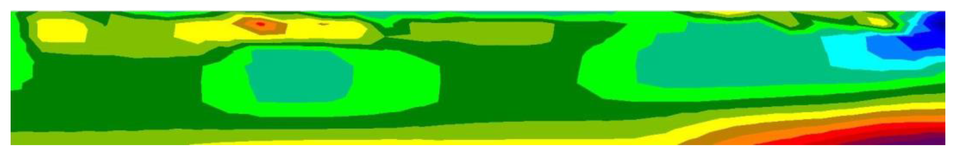
| AR | AR is Apparent Resistivity. |
| MSE | MSE is Mean Square Error. |
| PSNR | PSNR is Peak Signal to Noise Ratio. |
| SSIM [31] | SSIM is Structural Similarity Index Measure. |
| Dataset | Moving MNIST [34] | Caltech [36] | AR Map | ||||||
|---|---|---|---|---|---|---|---|---|---|
| MSE | PSNR | SSIM | MSE | PSNR | SSIM | MSE | PSNR | SSIM | |
| PredRNN++ [7] | 46.51 | 20.22 | 0.88 | 479.26 | 19.57 | 0.71 | 16.54 | 32.35 | 0.91 |
| DMLSTM | 49.66 | 20.53 | 0.90 | 437.65 | 20.14 | 0.72 | 18.45 | 32.78 | 0.90 |
| DA-PredRNN++ | 46.23 | 20.86 | 0.90 | 442.22 | 19.75 | 0.73 | 15.17 | 32.56 | 0.91 |
| DMANet | 44.36 | 21.36 | 0.91 | 423.98 | 20.46 | 0.74 | 13.14 | 33.16 | 0.92 |
| Dataset | Moving MNIST [34] | Caltech [36] | AR Map | ||||||
|---|---|---|---|---|---|---|---|---|---|
| MSE | PSNR | SSIM | MSE | PSNR | SSIM | MSE | PSNR | SSIM | |
| FRNN [14] | 69.76 ± 14.01 | 17.83 ± 1.91 | 0.81 ± 0.05 | 587.83 ± 251.22 | 16.43 ± 2.37 | 0.66 ± 0.11 | 25.48 ± 0.32 | 27.23 ± 0.41 | 0.86 ± 0.01 |
| PredRNN [6] | 58.82 ± 15.58 | 19.66 ± 1.86 | 0.86 ± 0.04 | 503.84 ± 259.64 | 18.83 ± 3.31 | 0.69 ± 0.10 | 19.81 ± 0.28 | 30.81 ± 0.31 | 0.89 ± 0.02 |
| PredRNN++ [7] | 46.51 ± 16.18 | 20.22 ± 1.64 | 0.88 ± 0.03 | 479.26 ± 245.43 | 19.57 ± 3.33 | 0.71 ± 0.10 | 16.54 ± 0.13 | 32.35 ± 0.34 | 0.91 ± 0.01 |
| MIM [18] | 45.24 ± 16.85 | 20.81 ± 1.72 | 0.91 ± 0.03 | 448.51 ± 232.67 | 20.12 ± 3.64 | 0.72 ± 0.09 | 14.27 ± 0.16 | 32.72 ± 0.37 | 0.92 ± 0.01 |
| DMANet | 44.36 ± 16.22 | 21.36 ± 1.67 | 0.91 ± 0.02 | 423.98 ± 233.71 | 20.46 ± 3.38 | 0.74 ± 0.09 | 13.14 ± 0.15 | 33.16 ± 0.36 | 0.92 ± 0.01 |
Publisher’s Note: MDPI stays neutral with regard to jurisdictional claims in published maps and institutional affiliations. |
© 2021 by the authors. Licensee MDPI, Basel, Switzerland. This article is an open access article distributed under the terms and conditions of the Creative Commons Attribution (CC BY) license (https://creativecommons.org/licenses/by/4.0/).
Share and Cite
Li, T.; Guan, Y. Dual Memory LSTM with Dual Attention Neural Network for Spatiotemporal Prediction. Sensors 2021, 21, 4248. https://doi.org/10.3390/s21124248
Li T, Guan Y. Dual Memory LSTM with Dual Attention Neural Network for Spatiotemporal Prediction. Sensors. 2021; 21(12):4248. https://doi.org/10.3390/s21124248
Chicago/Turabian StyleLi, Teng, and Yepeng Guan. 2021. "Dual Memory LSTM with Dual Attention Neural Network for Spatiotemporal Prediction" Sensors 21, no. 12: 4248. https://doi.org/10.3390/s21124248
APA StyleLi, T., & Guan, Y. (2021). Dual Memory LSTM with Dual Attention Neural Network for Spatiotemporal Prediction. Sensors, 21(12), 4248. https://doi.org/10.3390/s21124248