
Identification of the LLDPE Constitutive Material Model for Energy Absorption in Impact Applications

 ,
,  , , , , , and
Abstract
:1. Introduction
2. Materials and Methods

| Physical Properties | Unit | Tolerance ± | Value | Testing Method |
|---|---|---|---|---|
| Thickness | µm | 2 | 12 | Thickness gauge |
| Width | mm | 5 | 500 | Measuring tape |
| Length | - | 5 | High-speed encoder | |
| Density | - | 0.91–0.92 | ASTM D-1505 [23] | |
| Mechanical Properties | Unit | Tolerance± | Value | Testing Method |
| Tensile strength MD | MPa | 10 | 29.2 | ASTM D-882 [23] |
| Tensile strength TD | 14.1 | |||
| Break elongation MD | % | 245 | ||
| Break elongation TD | 540 | |||
| Dart drop | g | 40 | ASTM D-1709 [23] | |
| Puncture | kg | 1.7 | High-light tester | |
| Stretching level | - | - | 110 |
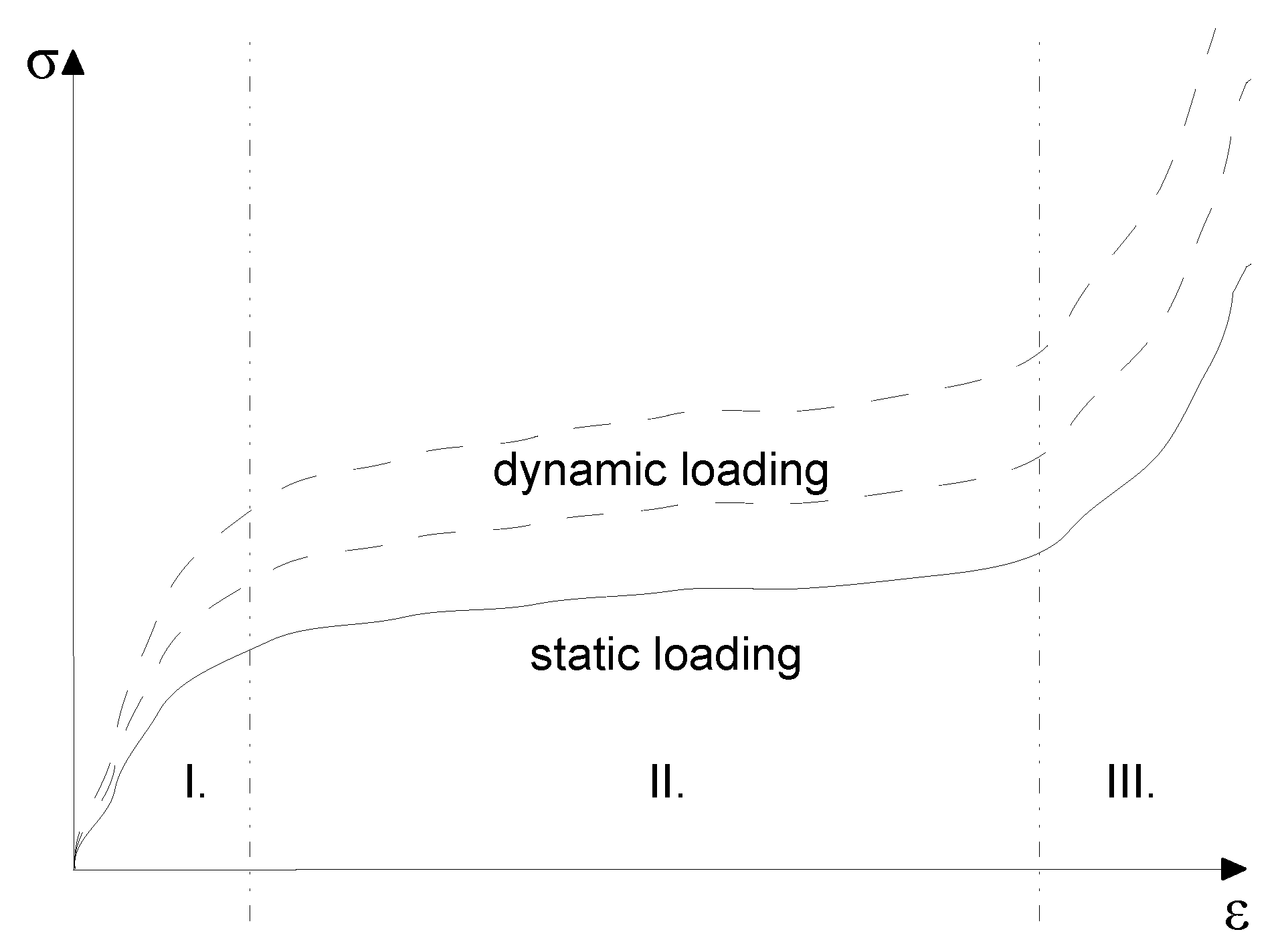
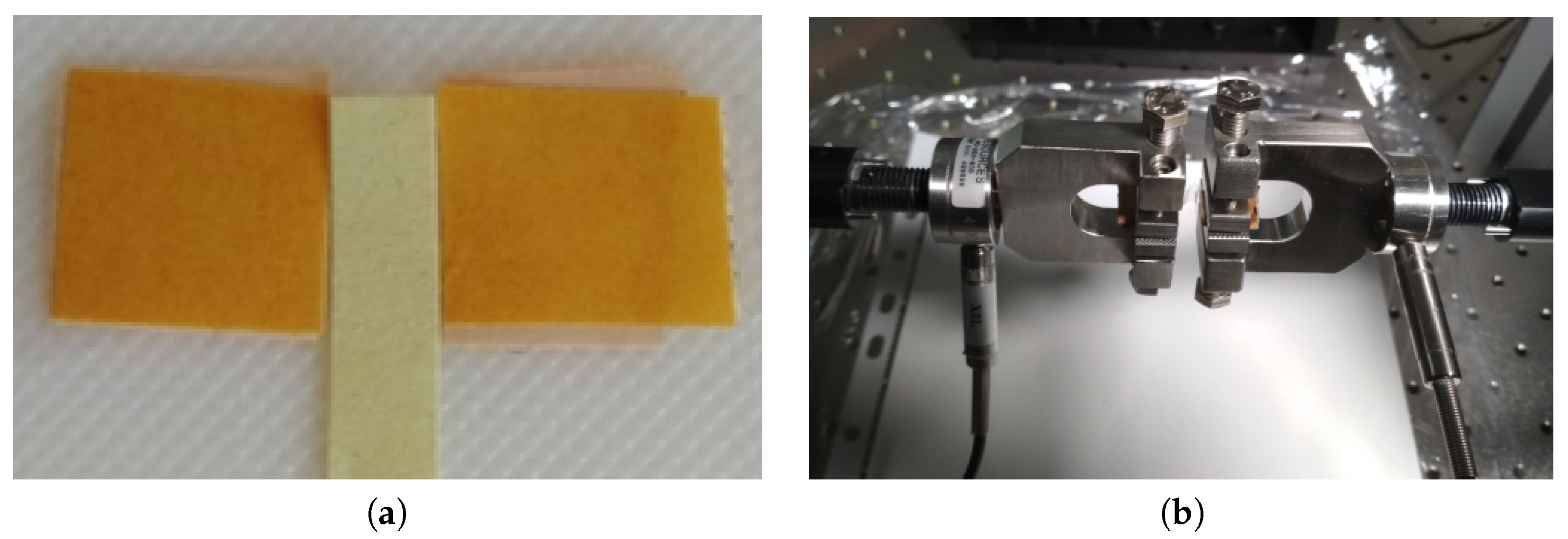
2.1. Quasi-Static Loading
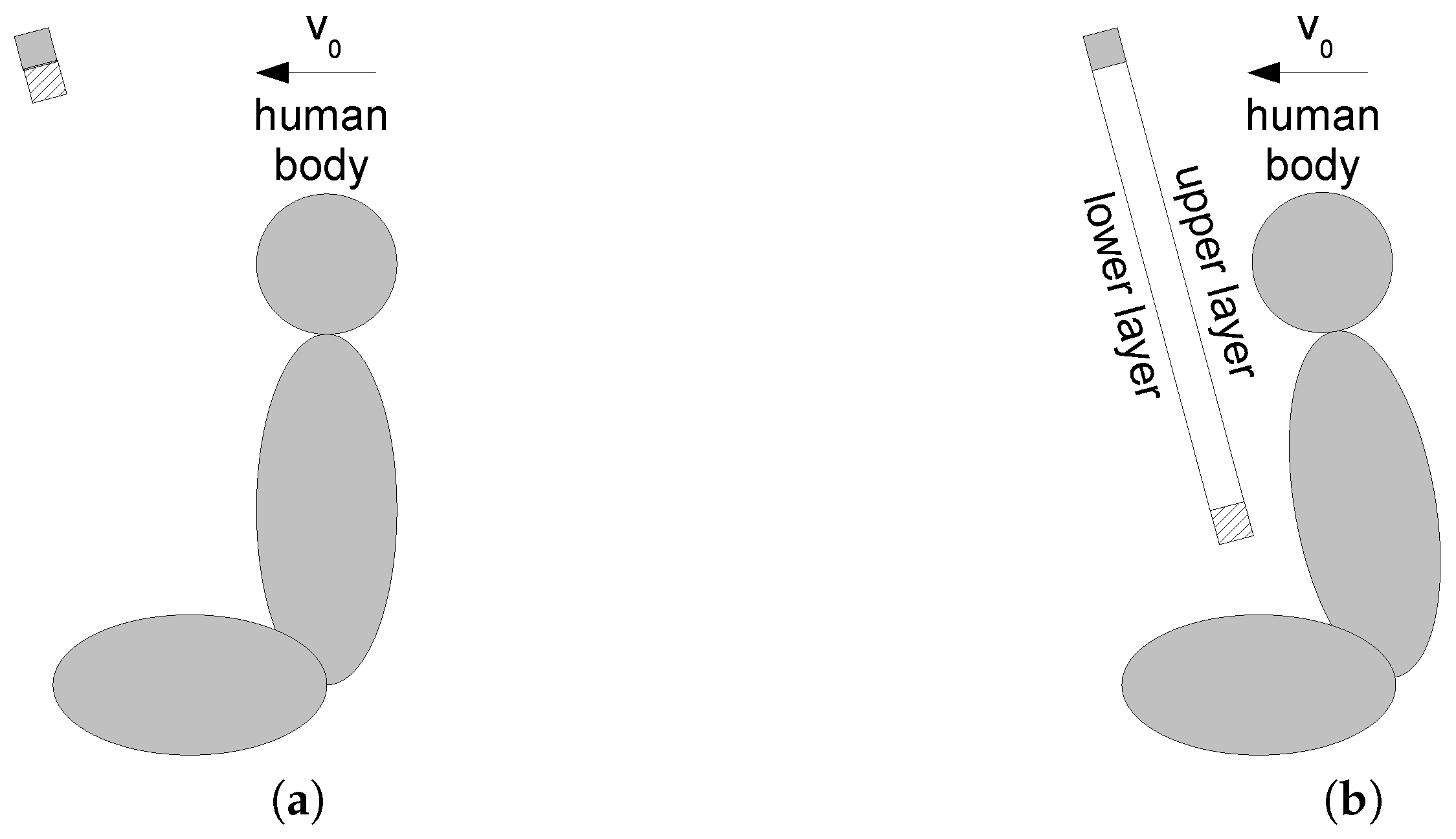
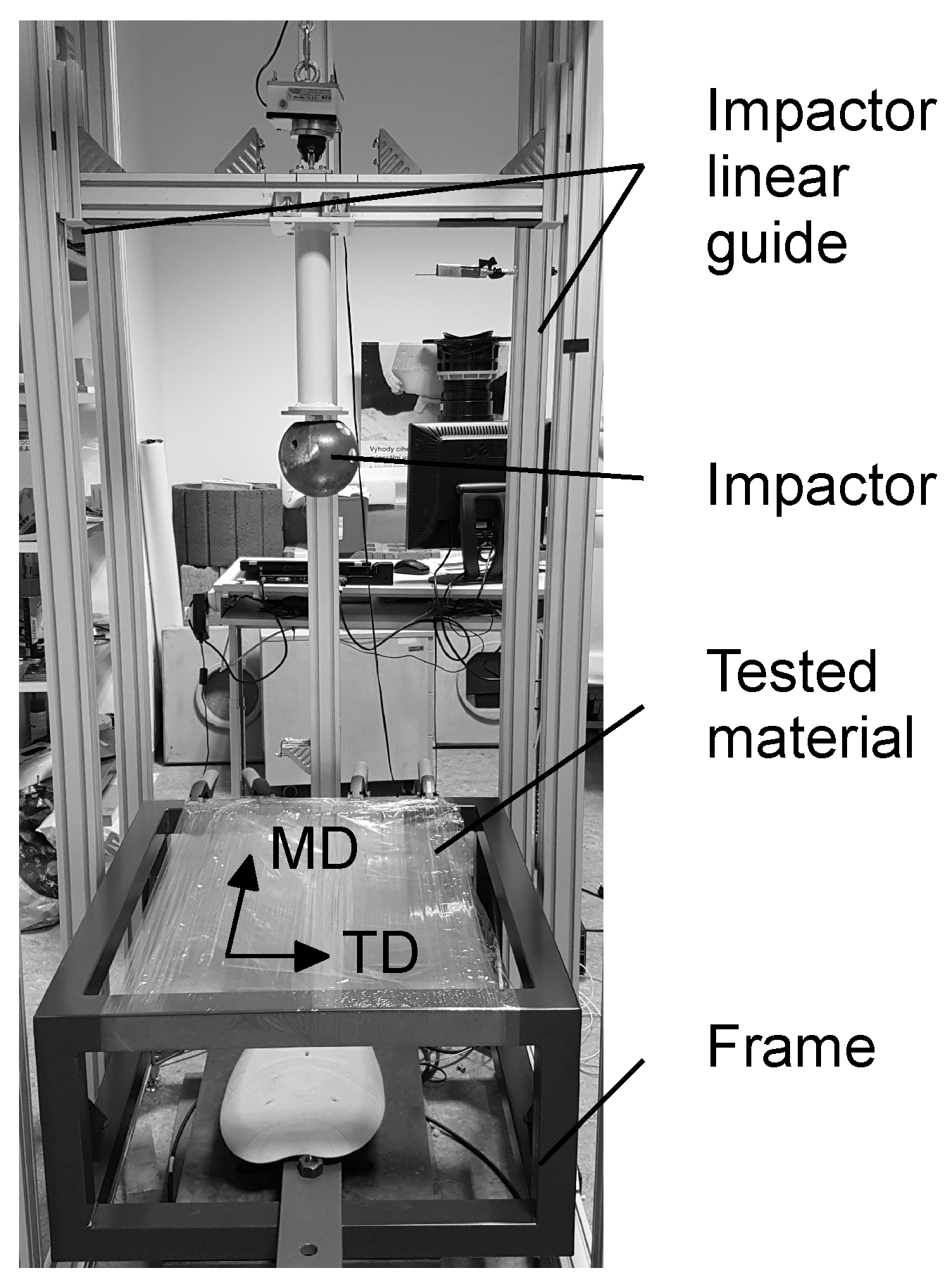
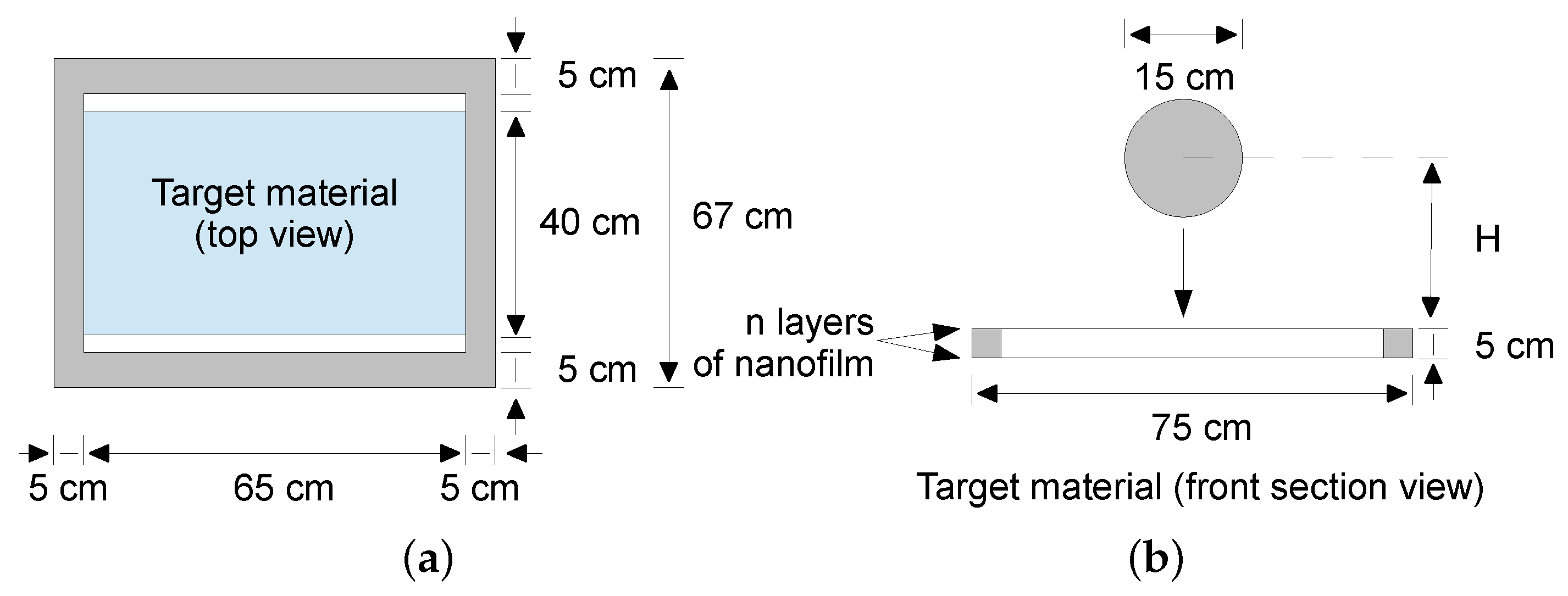
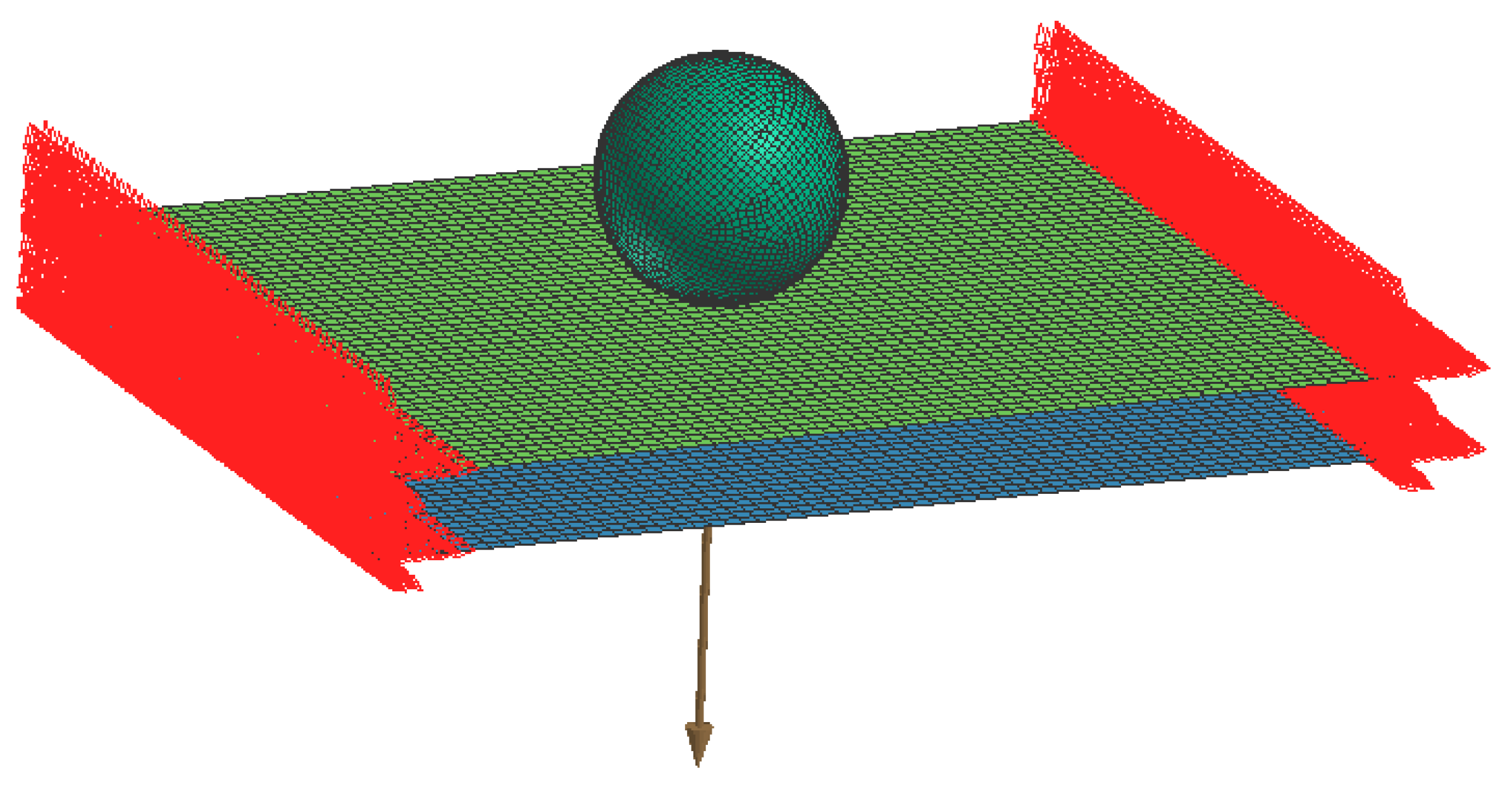
2.2. Dynamic Loading
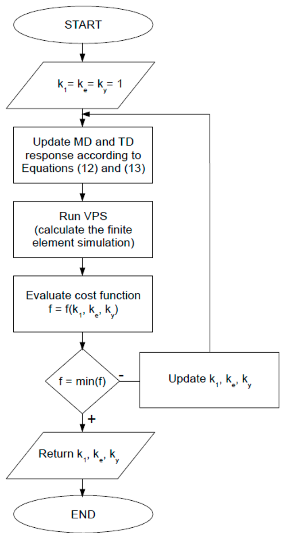
2.3. Identification of Dynamic Material Parameters
- Update both the MD and TD curves according to Equations (12) and (13):
- (a)
- update the stiffness by changing the slopes of the curves using ;
- (b)
- update the stiffness by changing the slopes of the curves using ;
- (c)
- update the resultant stress as ;
- (d)
- connect the parts of the curves in Regions II and III to the second yield point using and where is the shift of the second yield point;
- Run the VPS simulation to get for ;
- Evaluate the cost function f in Equation (16);
- Repeat the loop from 1 until the cost function f reaches its minimum;
- Return both the MD and TD curves according to Equations (12) and (13) for the optimized coefficients, , , and .
3. Results
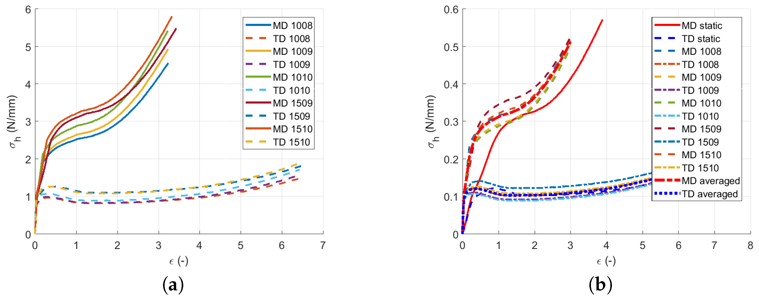
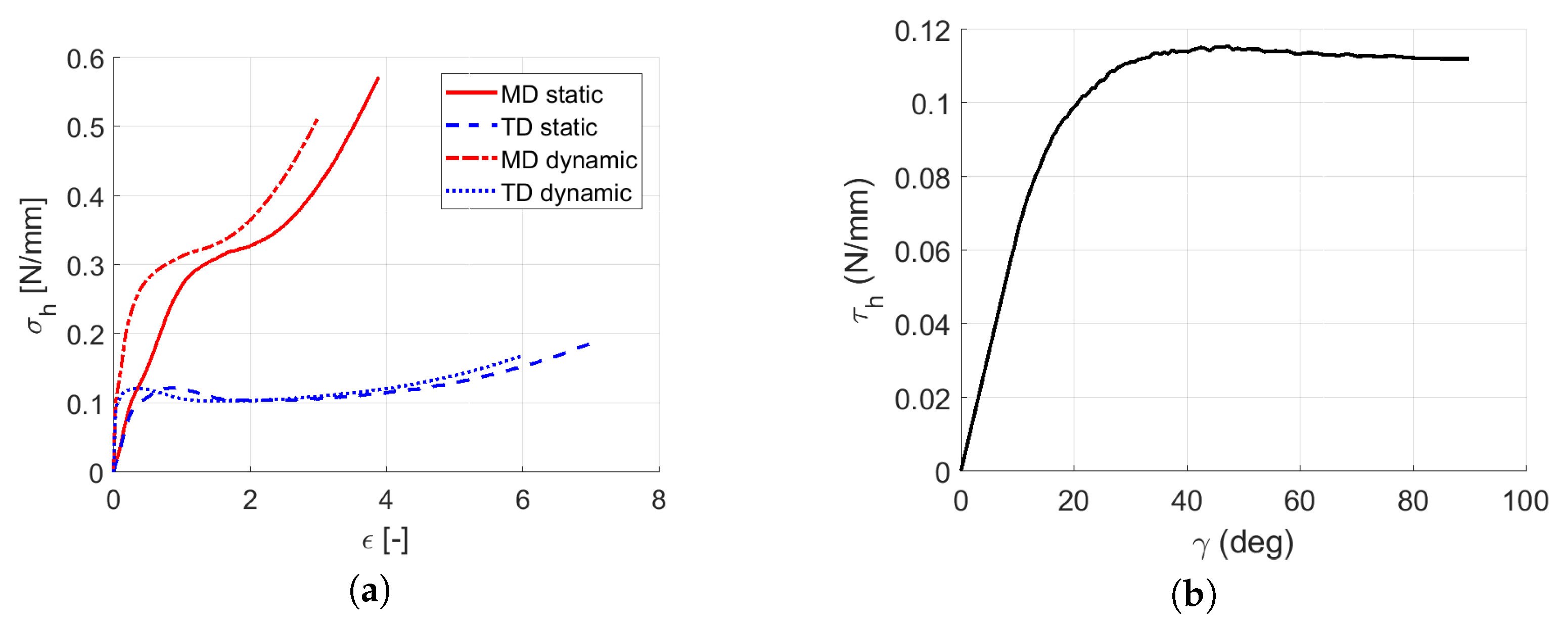
3.1. Quasi-Static Loading
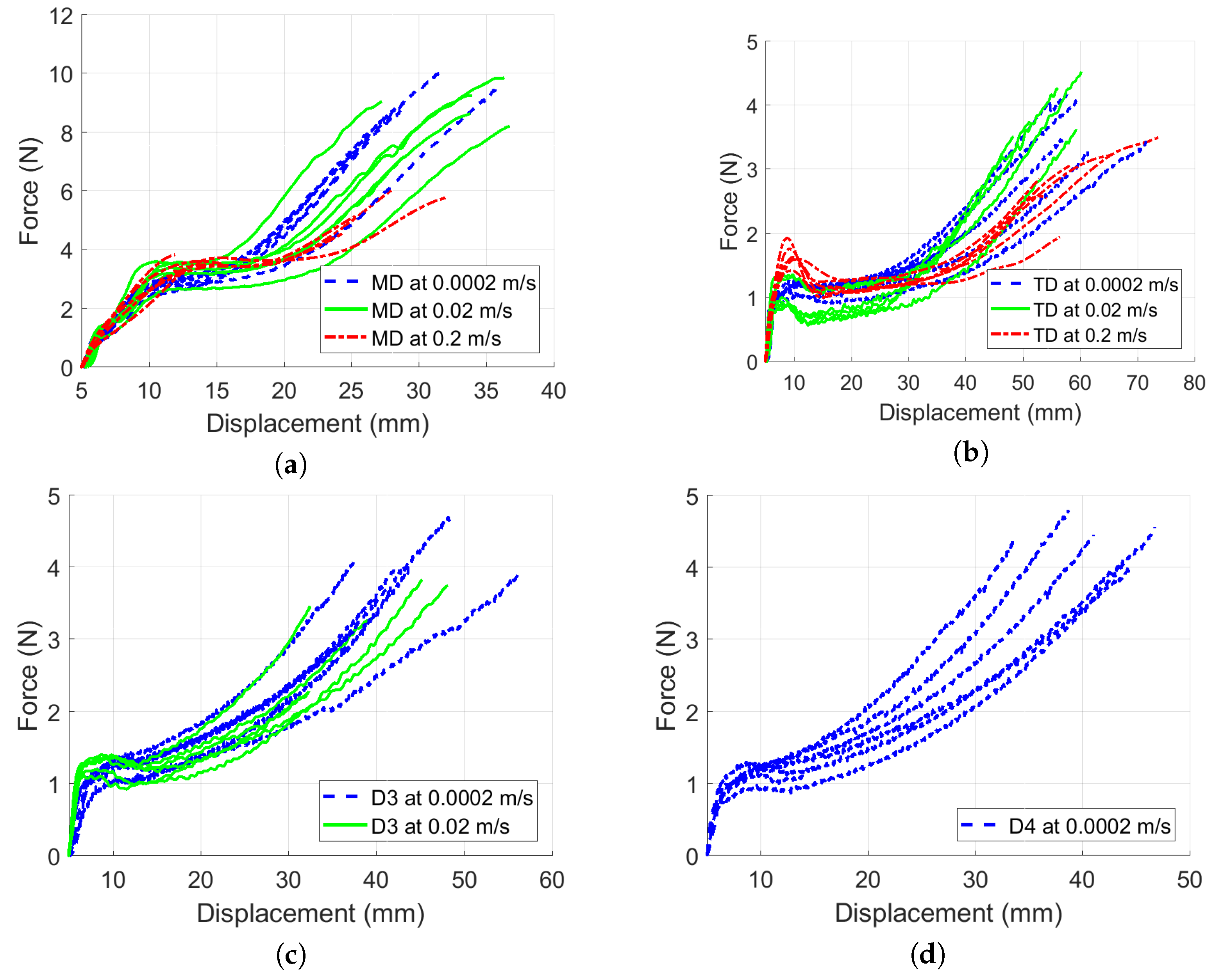
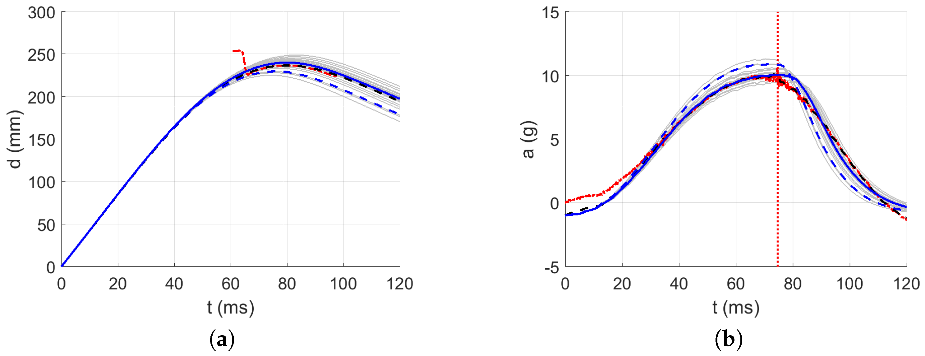
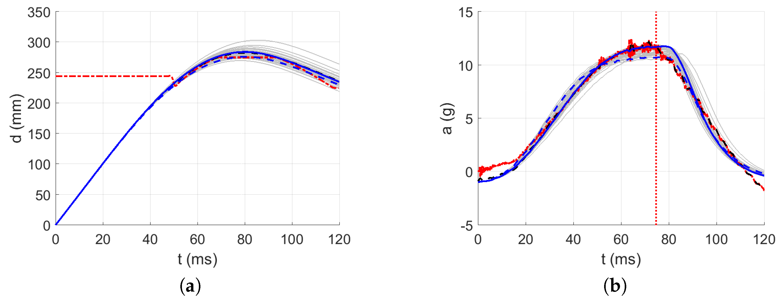
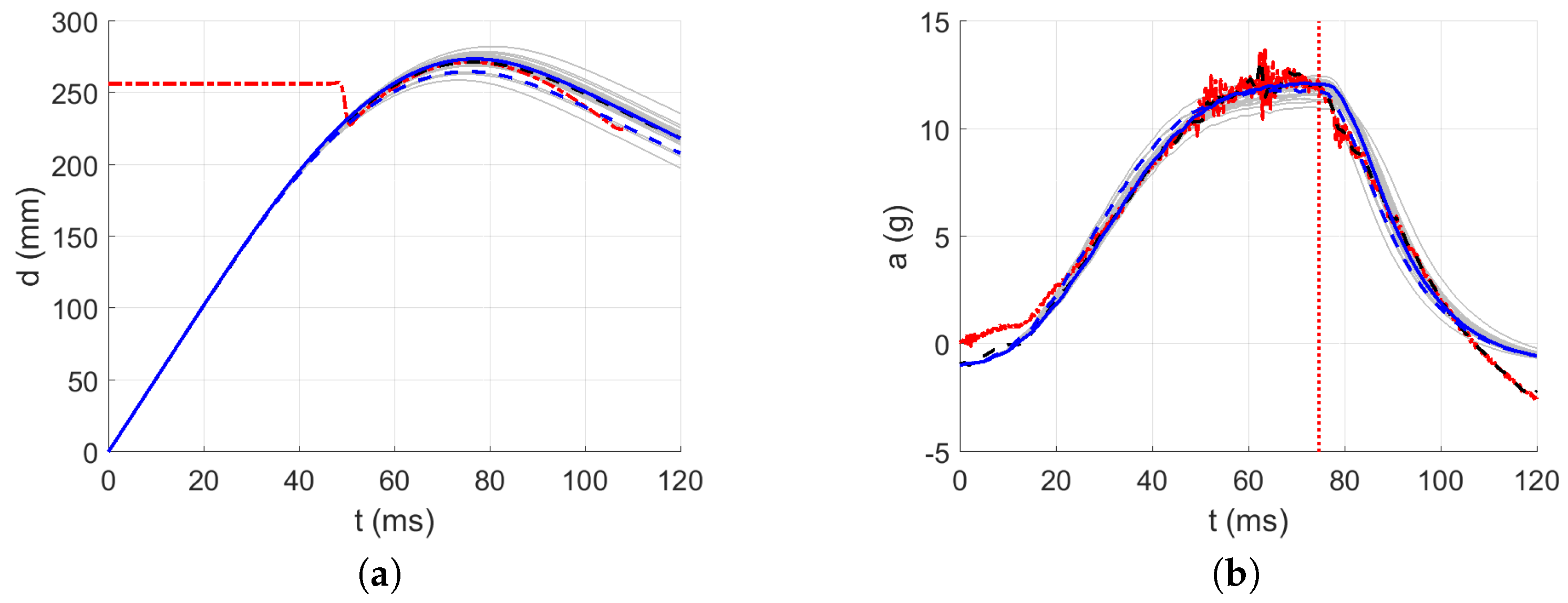
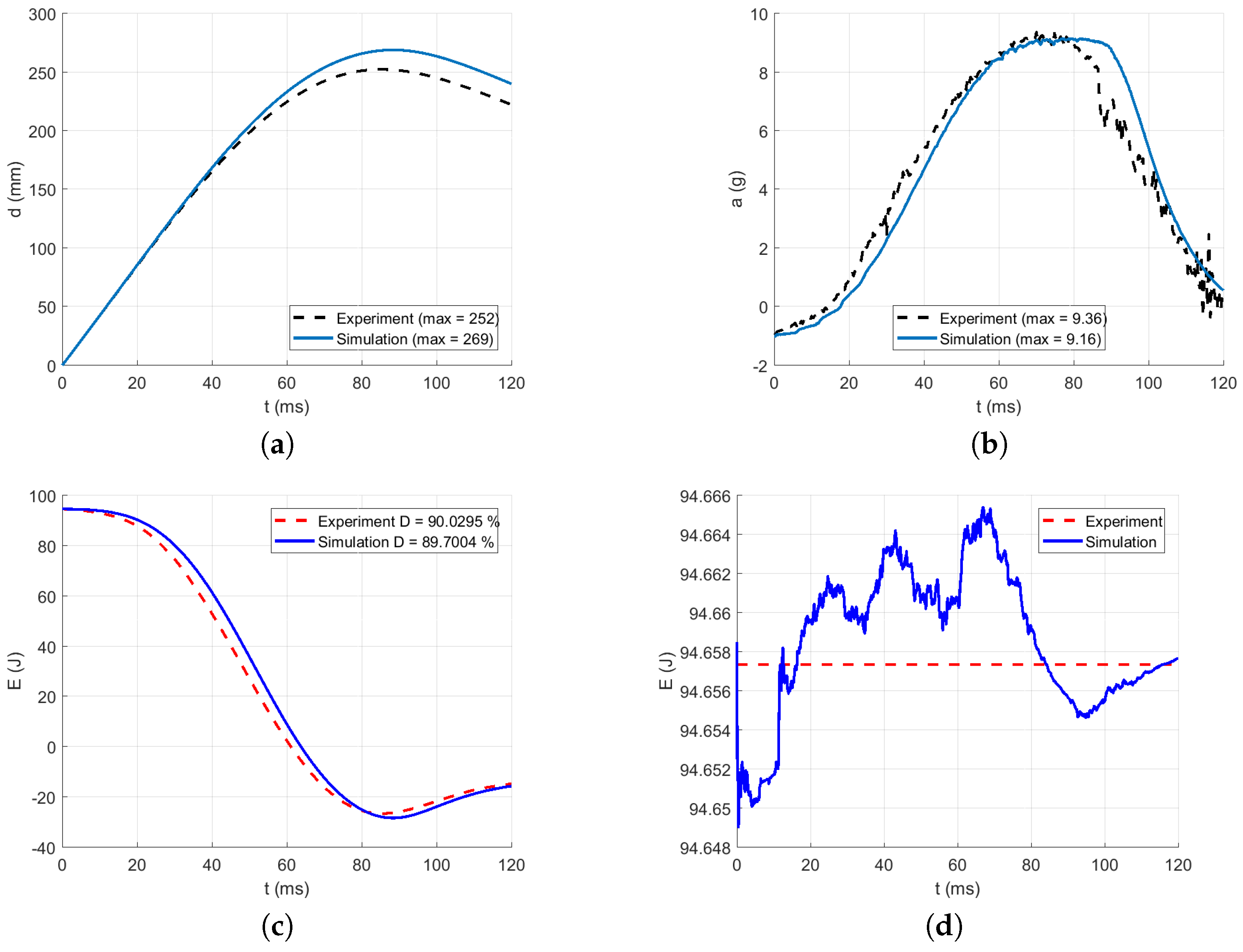
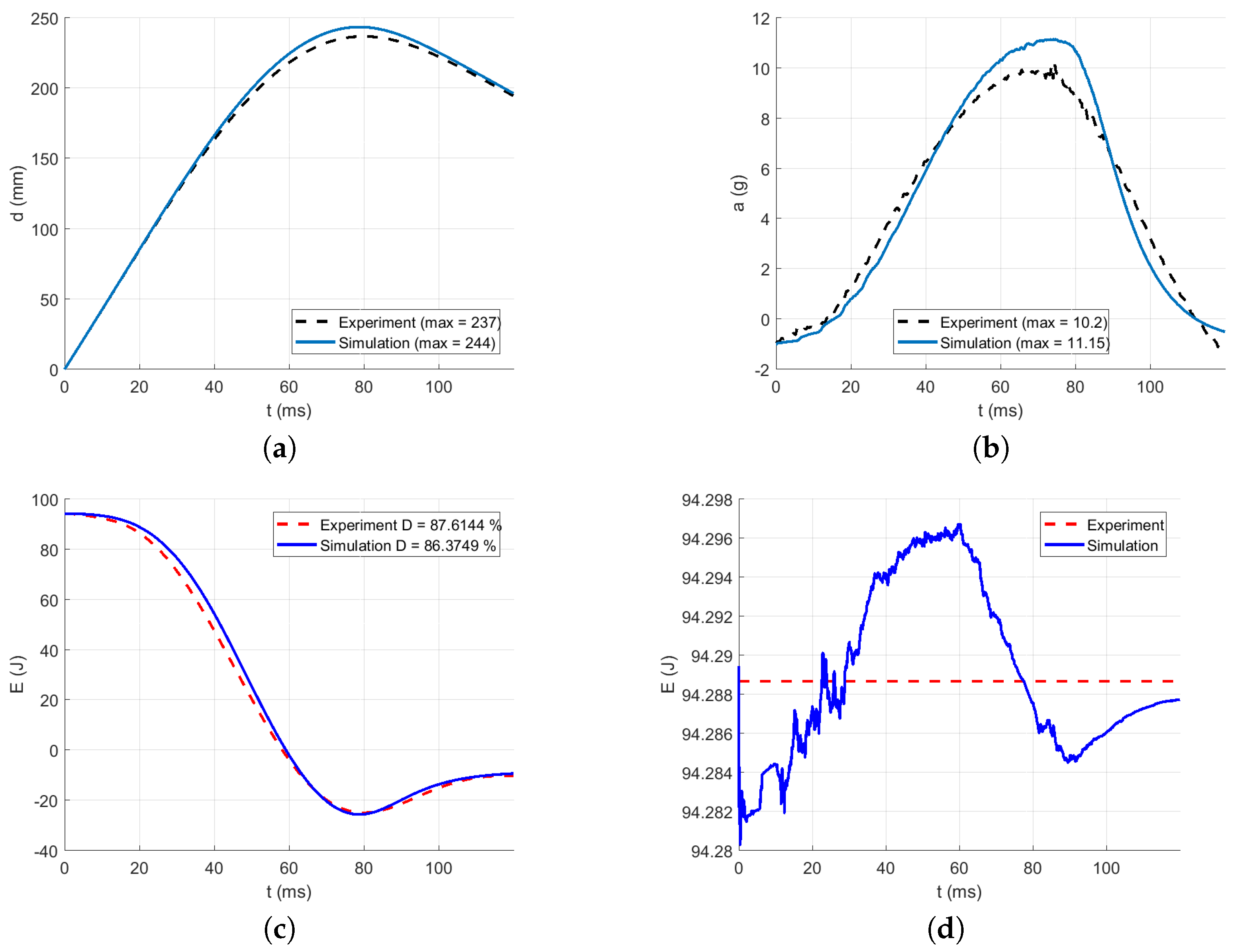
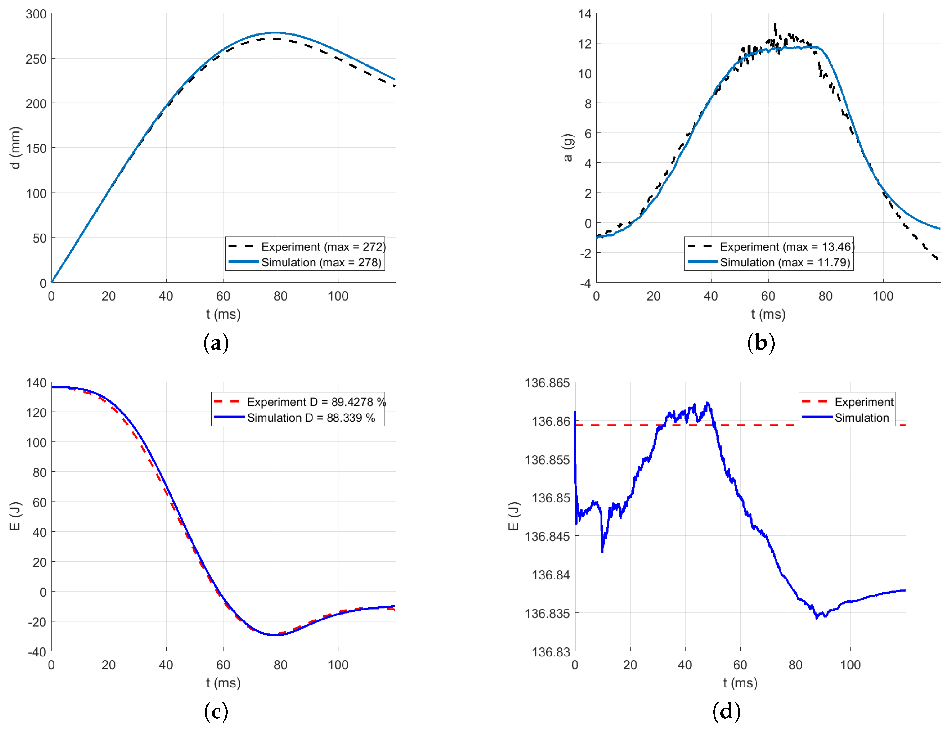
3.2. Dynamic Loading
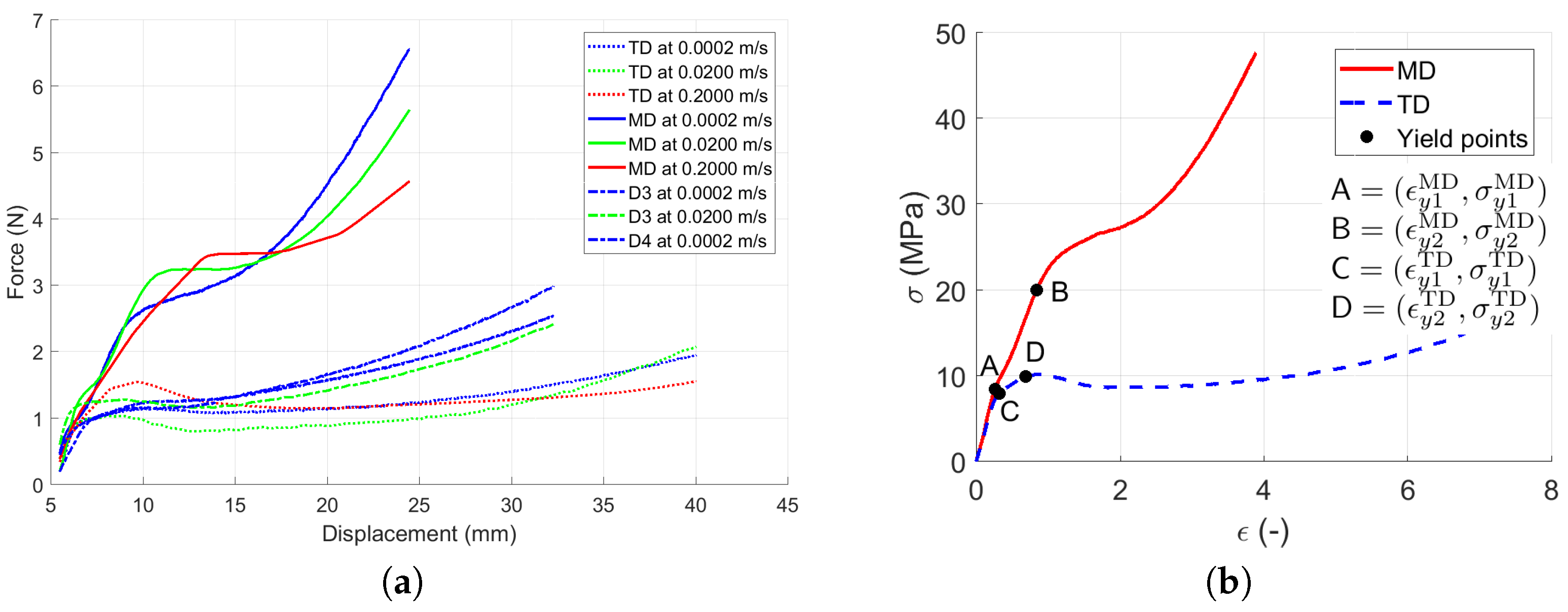
3.3. Identification of the Dynamic Material Parameters
4. Discussion
5. Conclusions
Author Contributions
Funding
Data Availability Statement
Acknowledgments
Conflicts of Interest
Abbreviations
| LLDPE | Linear low-density polyethylene |
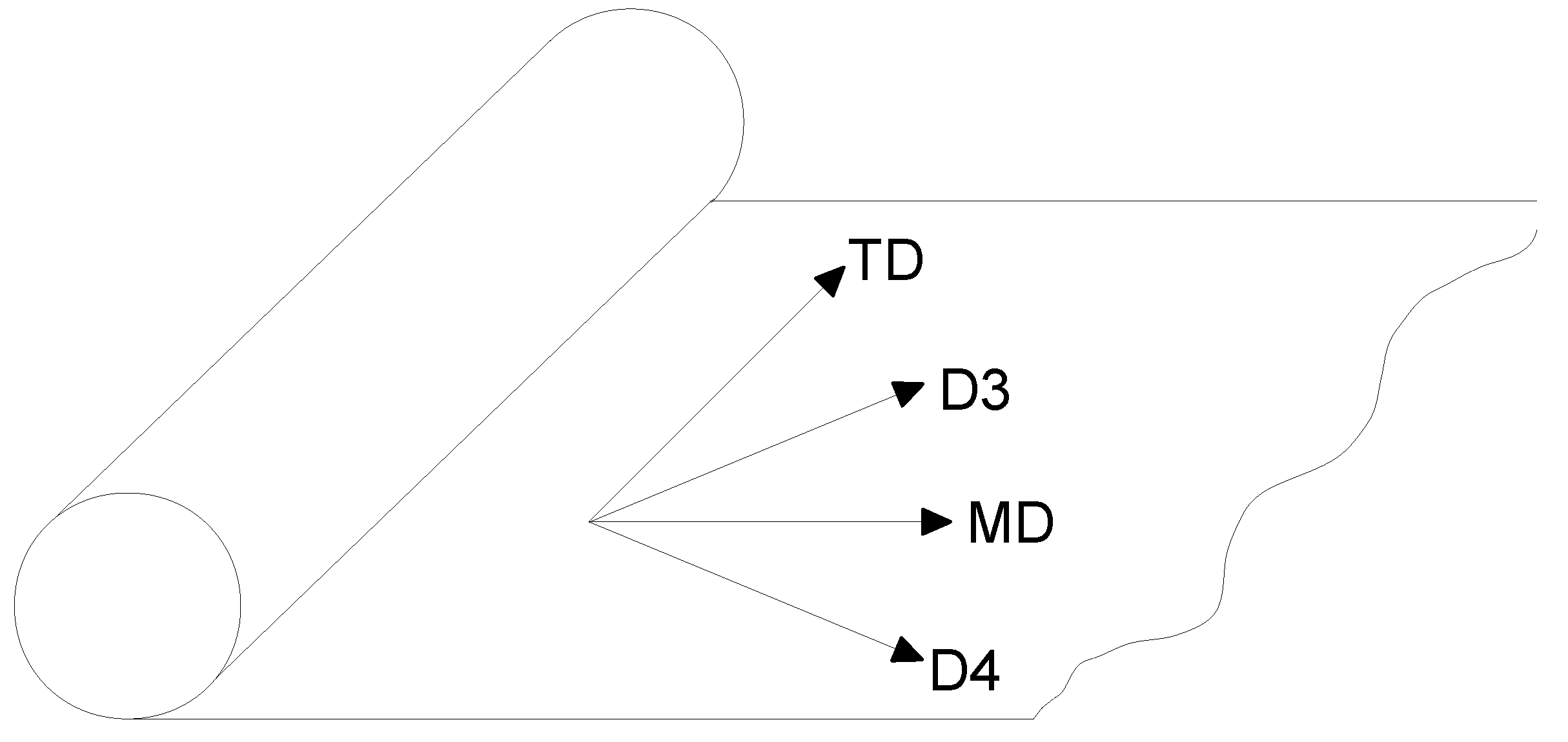
| MD | Machine direction |
| TD | Transverse direction |
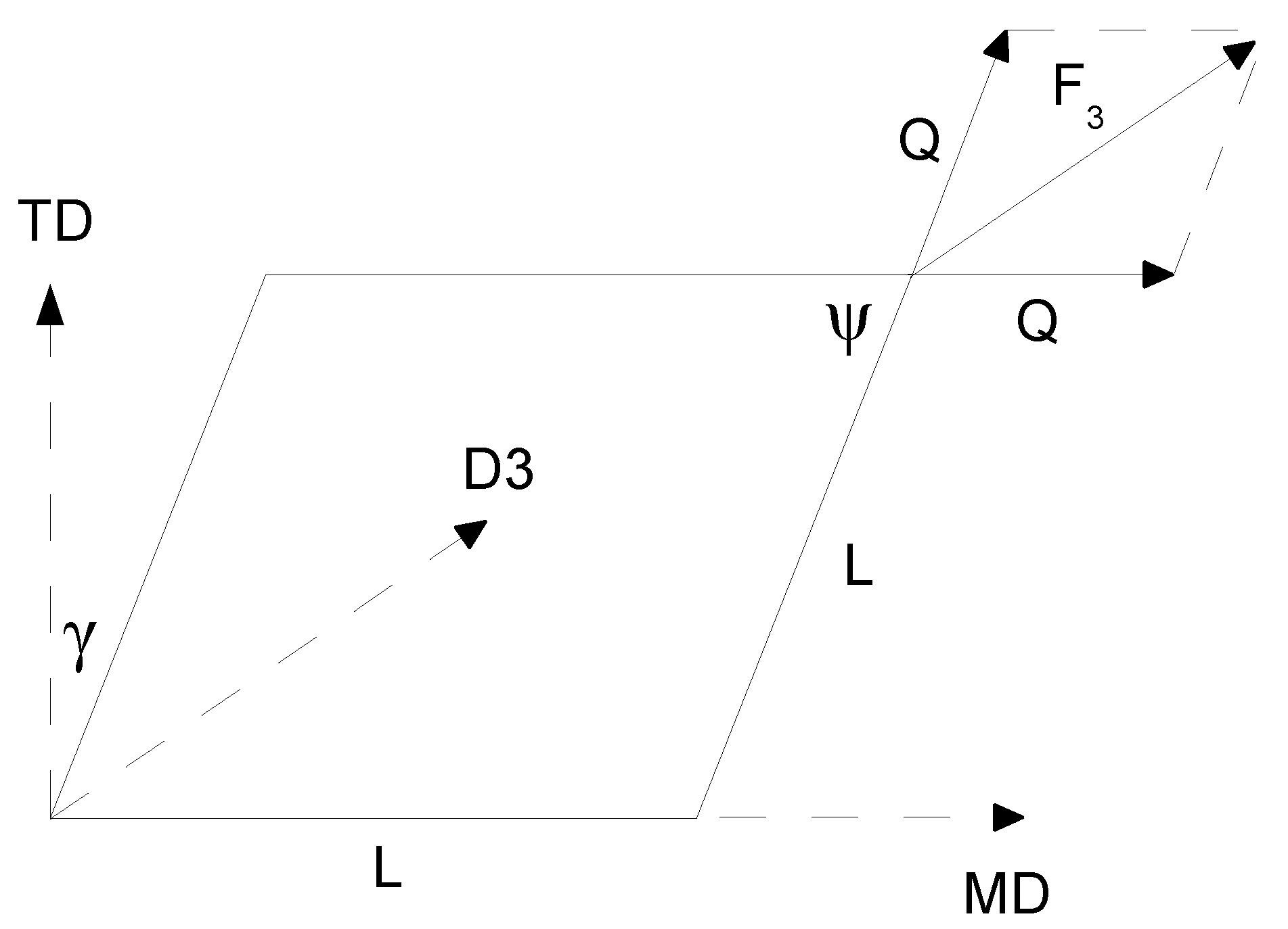
| D3 | Skewed direction by 45 |
| D4 | Skewed direction by −45 |
| VPS | Virtual Performance Solution |
Appendix A. Iteration Process Flowchart
Appendix B. List of Equations
References
- Špička, J.; Hynčík, L.; Kovář, L.; Hanuliak, A. Virtual assessment of advanced safety systems for new mobility modes. In Proceedings of the 16th International Symposium on Computer Methods in Biomechanics and Biomedical Engineering and the 4th Conference on Imaging and Visualization, New York, NY, USA, 14–16 August 2019; Columbia University: New York, NY, USA, 2019; p. 263. [Google Scholar]
- Hanuliak, A. Safety Restraint System for Motor Vehicles. WO2018/219371, 6 December 2018. [Google Scholar]
- Mezghani, K.; Furquan, S. Analysis of dart impact resistance of low-density polyethylene and linear low-density polyethylene blown films via an improved instrumented impact test method. J. Plast. Film. Sheeting 2012, 28, 298–313. [Google Scholar] [CrossRef]
- Ragaert, K.; Delva, L.; Van Damme, N.; Kuzmanovic, M.; Hubo, S.; Cardon, L. Microstructural foundations of the strength and resilience of LLDPE artificial turf yarn. Appl. Polym. Sci. 2016, 133, 1–12. [Google Scholar] [CrossRef] [Green Version]
- Bosi, F.; Pellegrino, S. Molecular based temperature and strain rate dependent yield criterion for anisotropic elastomeric thin films. Polymer 2017, 125, 144–153. [Google Scholar] [CrossRef] [Green Version]
- Bosi, F.; Pellegrino, S. Nonlinear thermomechanical response and constitutive modeling of viscoelastic polyethylene membranes. Mech. Mater. 2018, 117, 9–21. [Google Scholar] [CrossRef]
- Jeon, K.; Krishnamoorti, R. Morphological behavior of thin linear low-density polyethylene films. Macromolecules 2008, 49, 7131–7140. [Google Scholar] [CrossRef]
- Morris, B.A. Strength, stifffness, and abuse resistance. In The Science and Technology of Flexible Packaging; Elsevier: Oxford, UK, 2017; pp. 309–350. [Google Scholar]
- Omar, M.F.; Akil, H.M.; Ahmad, Z.A. Effect of molecular structures on dynamic compression properties of polyethylene. Mater. Sci. Eng. A 2012, 538, 125–134. [Google Scholar] [CrossRef]
- Jordan, J.; Casem, D.T.; Bradley, J.M.; Dwivedi, A.K. Mechanical Properties of Low Density Polyethylene. J. Dyn. Behav. Mater. 2016, 2, 411–420. [Google Scholar] [CrossRef] [Green Version]
- Zhang, X.M.; Elkoun, S.; Ajji, A.; Huneault, M.A. Oriented structure and anisotropy properties of polymer blown films: HDPE, LLDPE and LDPE. Polymer 2004, 45, 217–229. [Google Scholar] [CrossRef]
- Ren, Y.; Shi, Y.; Yao, X.; Tang, Y.; Liu, L.-Z. Different Dependence of Tear Strength on Film Orientation of LLDPE Made with Different Co-Monomer. Polymers 2019, 11, 434. [Google Scholar] [CrossRef] [Green Version]
- Dogru, S.; Aksoy, B.; Bayraktar, H.; Alaca, B.E. Poisson’s ratio of PDMS thin films. Polym. Test. 2018, 69, 375–384. [Google Scholar] [CrossRef]
- Dorigato, A.; Pegoretti, A.; Kolařík, J. Nonlinear tensile creep of linear low density polyethylene/fumed silica nanocomposites: Time-strain superposition and creep prediction. Polym. Compos. 2010, 31, 1947–1955. [Google Scholar] [CrossRef]
- Krishnaswamy, K.R.; Lamborn, M.J. Tensile Properties of Linear Low Density Polyethylene (LLDPE) Blown Films. Polym. Eng. Sci. 2000, 40, 2395–2396. [Google Scholar] [CrossRef]
- Plaza, A.R.; Ramos, E.; Manzur, A.; Olayo, R.; Escobar, A. Double yield points in triblends of LDPE, LLDPE and EPDM. J. Mater. Sci. 1997, 32, 549–554. [Google Scholar] [CrossRef]
- Richeton, J.; Ahzi, S.; Daridon, L.; Rémond, Y. Modeling of strain rates and temperature effects on the yield behavior of amorphous polymers. J. Phys. IV (Proc.) 2003, 110, 39–44. [Google Scholar] [CrossRef]
- Luyt, A.S.; Gasmi, S.A.; Malik, S.S.; Aljindi, R.M.; Ouederni, M.; Vouyiouka, S.N.; Porfyris, A.D.; Pfaendner, R.; Papaspyrides, C.D. Artificial weathering and accelerated heat aging studies on low-density polyethylene (LDPE) produced via autoclave and tubular process technologies. eXPRESS Polym. Lett. 2021, 15, 121–136. [Google Scholar] [CrossRef]
- Du, W.; Ren, Y.; Tang, Y.; Shi, Y.; Yao, X.; Zheng, C.; Zhang, X.; Guo, M.; Zhang, S.; Liu, L.Z. Different structure transitions and tensile property of LLDPE film deformed at slow and very fast speeds. Eur. Polym. J. 2018, 103, 170–178. [Google Scholar] [CrossRef]
- Omar, M.F. Static and Dynamic Mechanical Properties of Thermoplastic Materials; Lap Lambert Academic Publishing: Chisinau, Moldova, 2013. [Google Scholar]
- Durmus, A.; Kasgöz, A.; Macoscom, C.W. Mechanical Properties of Linear Low-density Polyethylene (LLDPE)/clay Nanocomposites: Estimation of Aspect Ratio and Interfacial Strength by Composite Models. Macromol. Sci. Part B Phys. 2008, 47, 608–619. [Google Scholar] [CrossRef]
- LLDPE Foils. 2020. Available online: http://www.tichelmann.cz/lldpe-folie (accessed on 21 November 2020).
- ASTM Standards. 2021. Available online: https://www.astm.org (accessed on 17 March 2021).
- ESI Group International. VPS User’s Manual; ESI Group International: Paris, France, 2020. [Google Scholar]
- Vezin, P.; Bruyère-Garnier, K.; Bermond, F.; Verriest, J.P. Comparison of Hybrid III, Thor-α and PMHS response in frontal sled tests. Stapp Car Crash J. 2002, 46, 1–26. [Google Scholar] [PubMed]
- Yoganandan, N.; Pintar, F.A.; Zhang, J.; Baisden, J.L. Physical properties of the human head: Mass, center of gravity and moment of inertia. J. Biomech. 2009, 42, 1177–1192. [Google Scholar] [CrossRef] [PubMed]
- Cichos, D.; de Vogel, D.; Otto, M.; Schaar, O.; Zoelsch, S.; Clausnitzer, S.; Vetter, D. Crash Analysis Criteria Description. 2011. Available online: http://mdvfs.org/crash-analyse (accessed on 9 May 2021).
- Gupalov, V.; Kukaev, A.; Shevchenko, S.; Shalymov, E.; Venediktov, V. Physical principles of a piezo accelerometer sensitive to a nearly constant signal. Sensors 2018, 18, 3258. [Google Scholar] [CrossRef] [PubMed] [Green Version]


| Stretching Velocity v (m/s) | Direction | Number of Samples N |
|---|---|---|
| MD | 6 | |
| TD | 6 | |
| D3 | 6 | |
| D4 | 6 | |
| MD | 6 | |
| TD | 6 | |
| D3 | 6 | |
| D4 | 6 | |
| MD | 6 | |
| TD | 6 | |
| D3 | 6 |
| Drop Height H (dm) | Number of Layers n | Optimization | Designation |
|---|---|---|---|
| 10 | 8 | √ | 1008 |
| 9 | √ | 1009 | |
| 10 | √ | 1010 | |
| 15 | 8 | × (material ruptured) | |
| 9 | √ | 1509 | |
| 10 | √ | 1510 | |
| Direction | MD | TD | ||
|---|---|---|---|---|
| Variable | Tensile Stress (MPa) | Break Elongation (%) | Tensile Stress (MPa) | Break Elongation (%) |
| Data sheet [22] | 29.2 | 245 | 14.1 | 540 |
| Experiment | 29.3 | 139 | 16.2 | 701 |
| Error (%) | 0.5 | −43 | 15 | 30 |
| Yield Point | MD | TD | ||||
|---|---|---|---|---|---|---|
| (-) | (MPa) | (N/mm) | (-) | (MPa) | (N/mm) | |
| 1 | 0.26 | 8.4 | 0.1 | 0.33 | 8 | 0.1 |
| 2 | 0.84 | 20 | 0.24 | 0.69 | 10 | 0.12 |
| Direction | MD | TD | ||||||||||
|---|---|---|---|---|---|---|---|---|---|---|---|---|
| Stretching Velocity v (m/s) | 0.0002 | 0.02 | 0.2 | 0.0002 | 0.02 | 0.2 | ||||||
| Young | 44 | 63 | 63 | 67 | 36 | 42 | 54 | 76 | 55 | 41 | 35 | 26 |
| modulus | 57 | 76 | 63 | 47 | 37 | 50 | 39 | 53 | 64 | 47 | 31 | 30 |
| E (MPa) | 63 | 41 | 81 | 70 | 31 | 30 | 55 | 44 | 49 | 58 | 27 | 38 |
| Young | 57 | 65 | 38 | 53 | 52 | 31 | ||||||
| modulus | 53 | 46 | ||||||||||
| E (MPa) |  | |||||||||||
| Drop Height H (dm) | 10 | 15 | |||
|---|---|---|---|---|---|
| Number of layers n | 8 | 9 | 10 | 9 | 10 |
| Impact velocity v (m/s) | 4.16 | 4.14 | 4.18 | 4.94 | 5.01 |
| Energy absorption D (%) | 90.03 | 88.26 | 87.61 | 89.13 | 89.43 |
| Energy absorption (%) | 88.63 | 89.28 | |||
 | |||||
| Drop Height H (dm) | 10 | 15 | |||
|---|---|---|---|---|---|
| Number of layers n | 8 | 9 | 10 | 9 | 10 |
| Number of iterations | 278 | 152 | 205 | 234 | 221 |
| First part stiffness multiplier (-) | 2.75 | 2.89 | 2.99 | 3.14 | 3.07 |
| Stiffness multiplier (-) | 3.41 | 3.47 | 3.55 | 1.69 | 2.29 |
| Yield stress multiplier (-) | 1.00 | 0.91 | 0.88 | 1.16 | 1.04 |
| Acceleration error (%) | 3 | 3 | 2 | 2 | 3 |
| Displacement error (%) | 1 | 1 | 1 | 0 | 1 |
| Drop Height H (dm) | 10 | 15 | |||
|---|---|---|---|---|---|
| Number of layers n | 8 | 9 | 10 | 9 | 10 |
| Acceleration error (%) | 6 | 8 | 10 | 6 | 3 |
| Displacement error (%) | 5 | 2 | 2 | 3 | 2 |
Publisher’s Note: MDPI stays neutral with regard to jurisdictional claims in published maps and institutional affiliations. |
© 2021 by the authors. Licensee MDPI, Basel, Switzerland. This article is an open access article distributed under the terms and conditions of the Creative Commons Attribution (CC BY) license (https://creativecommons.org/licenses/by/4.0/).
Share and Cite
Hynčík, L.; Kochová, P.; Špička, J.; Bońkowski, T.; Cimrman, R.; Kaňáková, S.; Kottner, R.; Pašek, M. Identification of the LLDPE Constitutive Material Model for Energy Absorption in Impact Applications. Polymers 2021, 13, 1537. https://doi.org/10.3390/polym13101537
Hynčík L, Kochová P, Špička J, Bońkowski T, Cimrman R, Kaňáková S, Kottner R, Pašek M. Identification of the LLDPE Constitutive Material Model for Energy Absorption in Impact Applications. Polymers. 2021; 13(10):1537. https://doi.org/10.3390/polym13101537
Chicago/Turabian StyleHynčík, Luděk, Petra Kochová, Jan Špička, Tomasz Bońkowski, Robert Cimrman, Sandra Kaňáková, Radek Kottner, and Miloslav Pašek. 2021. "Identification of the LLDPE Constitutive Material Model for Energy Absorption in Impact Applications" Polymers 13, no. 10: 1537. https://doi.org/10.3390/polym13101537