1. Introduction
Information from different surveys is mutually complementary, which makes it natural to consider a joint inversion of the data to a shared model, a process which can be implemented using several different physical and mathematical approaches. Integration of multiphysics data also helps reduce ambiguity, which is typical for geophysical inversions. Over the last decades, several approaches were introduced to joint inversion of geophysical data. The traditional technique is based on using the known petrophysical relationships between different physical properties of the rocks within the framework of the inversion process [
1,
2,
3,
4,
5,
6,
7,
8,
9]. The joint inversion can use these relationships or can indicate and characterize the existence of this correlation, yielding an improved final model.
Another approach to joint inversion uses a clustering concept from statistics, which assumes that the subsurface geology can be described by the models with petrophysical parameters forming a specific number of the known clusters in the space of the models (e.g., [
10,
11,
12]). This approach requires a priori knowledge of the parameters of these clusters, which is related to the lithology of the rocks.
In the cases where the model parameters are not correlated but nevertheless have similar geometrical features, joint inversion can be based on structure-coupled constraints. For example, these constraints can be implemented by the cross-gradient method, which enforces the gradients of the model parameters to be parallel [
13,
14,
15,
16,
17].
There still exist many challenges in incorporating typical geological complexity in joint inversion. For example, analytic, empirical, or statistical correlations between different physical properties may exist for only part of the shared earth model, and their specific form may be unknown. Features or structures that are present in the data of one geophysical method may not be present in the data generated by another geophysical method or may not be equally resolvable.
This review paper outlines and illustrates four novel approaches to joint inversion, which would not require a priori knowledge about specific empirical or statistical relationships between the different model parameters and/or their attributes. These approaches are designated as follows:
- (1)
Gramian constraints which enforce the correlation between different parameters. By imposing the requirement of the minimum of the Gramian mathematical operator in regularized inversion, we obtain multimodal inverse solutions with enhanced correlations between the different model parameters or their attributes.
- (2)
Joint inversion using Gramian-based structural constraints. In the framework of this approach, we apply the Gramian operator to the gradients of different model parameters; in this case, minimization of the Gramian results in enforcing the correlation between different gradients, which is equivalent to imposing the structural constraints.
- (3)
Localized Gramian constraints which impose local correlations between the various physical properties of the model, with changing parameters of these correlations within the modeling domain. In other words, the form of the relationships between different model parameters can change from one section of the inversion domain, with one type of lithological properties to another with different lithology. This is important in the case of complex geology.
- (4)
Joint focusing stabilizers, e.g., minimum support and minimum gradient support constraints. The joint focusing stabilizers force the anomalies of different physical properties to either overlap or experience a rapid change in the same spatial sector, thus enforcing the structural correlation.
In this paper, we review the mathematical principles of these four advanced approaches to joint inversion of multiphysics geophysical data and discuss some aspects of their applications. Considering the limited size of the journal paper, it would be impossible to provide the case studies for all four techniques covered in this review. The interested reader can find some examples of practical applications of these methods in several published papers, which are referenced in the sections below. At the same time, we have included, as an illustration, one example related to joint inversion of airborne magnetic and electromagnetic data using Gramian-based structural constraints. The reason for selecting this example is twofold. First, typical airborne geophysical surveys collect EM and magnetic data simultaneously; therefore, this pair of airborne datasets is readily available for many practical surveys. Second, this example clearly illustrates the benefits of joint inversion of the EM and magnetic data in mineral exploration.
2. Gramian Constraints
Gramian constraints enforce the correlation between different parameters or their transforms [
6,
7]. They are implemented by using a Gramian mathematical operator in regularized inversion, which results in producing multimodal inverse solutions with enhanced correlations between the different model parameters or their attributes. In this section, we present a short summary of the main principles underlying the Gramian regularization.
Let us consider forward geophysical problems for multiple geophysical data sets. These problems can be described by the following operator relationships:
where, in a general case,
is a nonlinear forward modeling operator;
are different observed data sets (which may have different physical natures and/or parameters); and
are the unknown sets of various physical properties (model parameters).
Note that diverse model parameters may have different physical dimensions (e.g., density is measured in g/cm
3, resistivity is measured in Ohm-m, etc.). It is convenient to introduce the dimensionless weighted model parameters,
where
is the corresponding linear operator of model weighting [
7].
It was demonstrated in [
6,
7] that one could apply the Gramian constraints to different transforms of the model parameters. For example, we may consider differential operations, like gradient, applied to the spatial distribution of the model parameters. This will result in the shared earth model characterized by similar behavior of the gradients of different physical properties. This type of the Gramian-based constraint is discussed in the next section of this review paper.
We can also use various functions of the model parameters, e.g., logarithms or trigonometric functions, to enforce the correlation between the transformed parameters. For example, in the case of joint gravity and seismic data inversion, one can use Gardner’s equation, which correlates the logarithm of density,
to the logarithm of velocity,
[
18]. In the case of joint EM and magnetic data inversion, one can consider the relationships between the logarithm of conductivity and magnetic susceptibility. This example will be provided in the final section of the paper.
Joint inversion of multiphysics data can be reduced to minimization of the following parametric functional,
where misfit functionals,
are defined as follows,
and
are the weighted predicted data:
where
is the corresponding linear operator of data weighting.
The selection of the model and data weights was discussed in many publications on inversion theory. For example, in the framework of the probabilistic approach [
19], the weights were determined as inverse data covariance or model covariance matrices. In the framework of the deterministic approach [
20], the weights were determined as inverse integrated sensitivity matrices.
In Formula (2),
is a stabilizing functional. This functional can be introduced as a determinant of the Gram matrix of a system of model parameters,
,
, …,
, which is called a Gramian,
S =
[
6,
7].
Gramian provides a measure of correlation between the different model parameters or their attributes. By imposing an additional requirement minimizing the Gramian in regularized inversion, we obtain multimodal inverse solutions with enhanced correlations between the various model parameters.
For example, in the case of two model parameters (e.g., density and magnetic susceptibility), the Gramian is computed as follows:
where (⋅,⋅) stands for the inner product in the corresponding Hilbert space of model parameters [
7].
In a general case of
n model parameters, the Gramian is computed as the determinant of the Gram matrix as follows:
Note that, in Equation (6) and everywhere below we drop the “tilde” sign above the model parameters to simplify the notations. However, we still consider being the dimensionless weighted or transformed model parameters.
The main property of the Gramian in Equation (6) is that it is a nonnegative functional, and the Gramian is equal to zero if the model parameters, are linearly dependent.
One can also choose various metrics of the Hilbert space in Equation (6), used in the definition of the Gramian [
7]. This brings additional flexibility to the type of coupling between different model parameters enforced by the Gramian constraints, which is illustrated below.
The meaning of Gramian and its role in the joint inversion can be better explained using a probabilistic approach to inverse problem solution. In the framework of this approach, one can treat the observed data and the model parameters as the realizations of some random variables [
19,
20].
We can also introduce a Hilbert space with the metric defined by the covariance between random variables, representing different model parameters. Under these assumptions, the Gramian stabilizing functional arises as a determinant of the covariance matrix between different model parameters [
21]:
In the last formula,
represents a covariance between two random variables,
and
, describing two different physical properties of the inverse model. Note that the covariance of a datum with itself is just the variance:
where
is the standard deviation of model parameter,
For example, in a case of two model parameters, we have
where
and
are standard deviations of the random variables corresponding to parameters
, respectively, and coefficient
η is a correlation coefficient between these two parameters:
The last expression shows that the Gramian provides a measure of correlation between two parameters, and . Indeed, the Gramian goes to zero when the correlation coefficient is close to one, which corresponds to linear correlation. This property shows that, by imposing the Gramian constraint, we enforce a linear correlation between the model parameters.
The same property holds in the multiphysics case where we have n different physical property parameters. The minimization of the determinant of the covariance matrix shown in Equation (7) results in enforcing the linear correlations between those parameters.
Case studies of practical applications of the Gramian constraints have been presented in several recently published papers. For example, Malovichko et al. [
22] demonstrated how Gramian constraints can be used for guided full-waveform inversion of seismic data using known petrophysical properties of the rocks. In the papers [
23,
24], the authors applied Gramian constraints in joint inversion for density and magnetization models. We refer interested readers to these publications for more details on technical applications of the Gramian approach.
We have demonstrated above that Gramian approach is based on the concept of linear correlation; however, by applying this concept to the transforms of the model parameters, we can amplify a variety of different properties in joint inversion. For example, Gramian of the gradients of the model parameters results in structural correlations. Gramian applied to the nonlinear transforms of the model parameters results in nonlinear correlations. Gramian applied locally (in the framework of the localized approach) results in spatially variable relationships between different physical properties. In short, the Gramian approach is not limited to a strict linear correlation assumption. This property of Gramian approach will be illustrated below in the sections dedicated to the structural and localized Gramian-based constraints.
3. Joint Inversion Using Gramian-Based Structural Constraints
One of the most widely used approaches to imposing the structural constraints on the results of the joint inversion is based on the method of cross gradients [
13,
14,
15,
16,
17]. The basic idea behind this method is that the gradients of the model parameters should be parallel in order to enforce the geometrical similarities between the interfaces of the models. Within the framework of the cross-gradient method, this requirement can be achieved by minimizing the norm square of the cross product of the gradients of these functions:
One of the problems of the practical implementation of this method is related to the fact that the cross-gradient functional is non-quadratic, which makes it challenging to find the Fréchet derivative of this functional; it is a non-trivial task to extend the method to more than two types of data, e.g., seismic, gravity, and electromagnetic. At the same time, the Gramian stabilizing functional is always quadratic, as the conventional minimum norm functional [
7]. This makes it easier to calculate the derivatives of the Gramian functional and provides the basis for a relatively simple numerical implementation.
In the framework of the Gramian approach, the same requirement for the gradients of the model parameters being parallel is achieved by minimizing the structural Gramian functional,
, which, in a case of two physical properties, can be written using matrix notations, as follows:
By minimizing the Gramian functional,
, we enforce the linear correlation between the gradients of the model parameters, making these vectors parallel to each other. The method can also be naturally expanded for any number,
n, of the model parameters, by considering the corresponding Gramian matrices between the gradients of the different parameters. The practical advantage is, again, in the quadratic nature of this functional, which was demonstrated in [
6,
7]. This property was proved based on the concept of the Gramian space which was shown to be a Hilbert space with all related useful properties.
For example, we can introduce a stabilizing term in the parametric functional shown in Equation (2) as a superposition of the structural Gramians between the first and all other physical model parameters:
Minimization of the expression in the right-hand side of Equation (13) keeps all gradient vectors, , parallel to each other. Considering that the gradient directions are orthogonal to the interfaces between the structures with contrasting physical properties, this condition results in structural similarities between the inverse models describing different physical properties of the earth.
Practical applications of the Gramian-type structural constraints were presented in papers [
25,
26,
27], among others. Jorgensen and Zhdanov [
26] applied this approach to imaging the deep magma-feeding structure of the Yellowstone supervolcano by joint inversion of gravity and MT data. In paper [
27], this technique was used for joint inversion of the gravity and magnetic data collected over the Thunderbird V-Ti-Fe deposit in the Ring of Fire area of Ontario, Canada. The cited papers also contain a detailed description of the numerical algorithm of minimizing the parametric functional shown in Equation (2) with the Gramian structural stabilizer shown in Equation (12).
4. Localized Gramian Constraints
The constraints based on minimization of the Gramian of the model parameters, Equations (5) and (6), or of their gradients, Equations (12) and (13), can be treated as the global constraints, because they enforce similar correlation conditions over the entire inversion domain. In practical applications, however, the specific form of the correlations may vary within the area of investigation. To address this situation, we can subdivide the inversion domain,
D, into
N subdomains,
, with potentially different types of relationships between the different model parameters, and define the Gramians,
for each of these subdomains separately:
where
, are the sets of model parameters describing the different physical properties of the medium (e.g., density, susceptibility, or conductivity) within subdomain
.
In this case, the localized Gramian constraints will be based on using the following stabilizing functional:
In a similar way, we can introduce localized Gramian-based structural constraints, using the localized Gramian of model parameter gradients,
, defined by the following formula:
For example, in a case of two model parameters, localized Gramian (16) takes the form:
and the corresponding stabilizing functional is written as follows:
The advantage of using the localized Gramian constraints over the global constraints is that the former can be applied in complex geological settings with variable relationships between different physical properties of the rock formations over the area of investigation. Note that one can use an individual discretization cell, of the inversion domain as an elementary subdomain, to achieve the maximum flexibility of the localized constraints. In the case of Gramian structural constraints, the corresponding localized constraint will require the gradients of the different model parameters to be parallel (linearly dependent) vectors within every cell, while allowing for the coefficients of the linear dependence to vary from cell to cell. This provides more flexibility to the joint inversion.
Paper [
28] presents a case study of jointly inverting the gravity and seismic data collected in Yellowstone National Park using localized Gramian constraints. The cited paper also addresses the important issue of dealing with different resolution capabilities of various geophysical methods in joint inversion. Interested readers can find useful practical details in [
28] for applying this technique to image the crustal magmatic system of Yellowstone.
5. Joint Focusing Constraints
The structural similarities between various petrophysical models of the subsurface can be enforced by using the joint total variation or focusing stabilizers [
29,
30]. For the solution of a nonlinear inverse problem shown in Equation (1), following [
29,
30], we introduce the following parametric functional with focusing stabilizers,
where the terms
, and
are the joint stabilizing functionals, based on minimum support, and minimum gradient support constraints, respectively.
The joint minimum support stabilizer,
is proportional to the combined volume, or support, occupied by domains with anomalous physical parameters for small
e.
Indeed, we can rewrite Equation (20) as follows:
In Equation (21) we denote by , a joint support of , which is defined as a volume of the combined closed subdomain of V where all
From Equation (21), one can find immediately that
Thus, is proportional to the combined anomalous model parameters support for a small e.
It can be easily established by a simple geometrical analysis that the combined anomalous model parameters support reaches the minimum when the volumes occupied by anomalous domains representing various physical properties coincide. Indeed, if the anomalous properties are in different locations, their combined support is larger in comparison to cases when the locations are the same.
A joint minimum gradient support functional (JMGS) is defined as follows:
Repeating the algebraic transformation presented in expression (21), one can demonstrate that:
where
a joint support of the gradients of various anomalous model parameters,
Therefore,
is proportional to the joint support of the gradients of different properties of the rocks. It is obvious that these gradients are directed perpendicular to the interfaces between different lithologies and they achieve the maximum values at these interfaces. By imposing the minimum joint gradient support constraint, we force the interfaces expressed in diverse petrophysical parameters to merge, thus ensuring a structural similarity of the multiphysics inverse problem solutions. The geometrical explanation of this fundamental property of the JMGS functional is the same as for the case of the JMS functional, discussed above.
The minimization of the parametric functional shown in Equation (19) is based on the re-weighted regularized conjugate gradient method (RRCG) [
7], which iteratively updates the model parameters to minimize the parametric functional and the misfit between the observed and predicted data. The inversion iterates until the misfit reaches a given threshold.
Examples of practical application of this approach can be found in [
27,
29,
30].
6. Case Study: Joint Inversion of EM and TMI Data of the Reid-Mahaffy Test Site, Ontario
In this section, we present an example of joint inversion of magnetic and electromagnetic data collected in the Reid-Mahaffy test site using Gramian-based structural constraints. As we have explained above in
Section 3, the Gramian-based structural constraints require the gradients of the various physical properties to be parallel to each other. It is well known that the gradients are directed perpendicular to the interfaces between the areas with different physical properties. By requiring the gradients to be parallel, we enforce the structural similarities between the models representing diverse physical properties. In the present case study, we apply the joint inversion to airborne electromagnetic (AEM) and total magnetic intensity (TMI) data collected by geophysical surveys in the Reid-Mahaffy test site. The AEM data reflect the conductivity distribution in the subsurface, while the TMI data manifest magnetic properties of the rocks. Assuming that various rock formations are characterized by distinct electrical and magnetic properties, we expect that the joint inversion of AEM and TMI data using the Gramian-based structural constraints will better resolve the complex geological structure of the surveyed area than the standalone inversions.
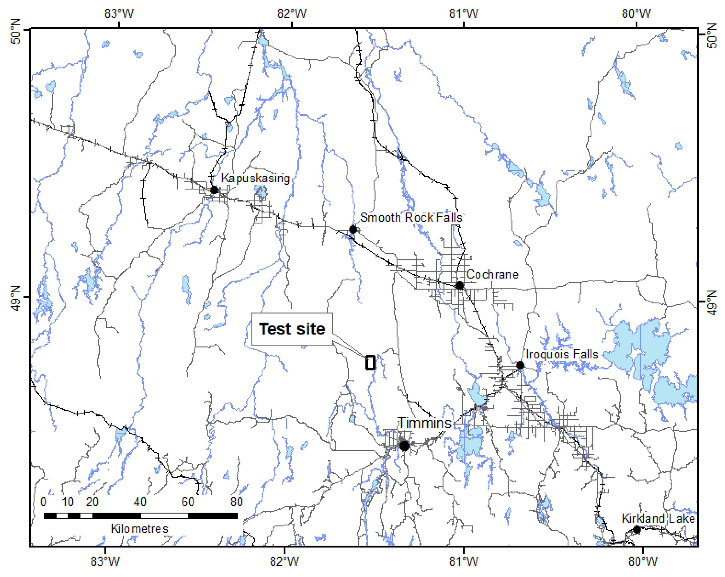
The Reid-Mahaffy test site is located in the Abitibi Subprovince, immediately east of the Mattagami River Fault (
Figure 1). The test site was created in 1999 by the Ontario Geological Survey as part of Operation Treasure Hunt, a multi-year geoscientific program intended to increase the precompetitive perspectivity of Ontario for precious and base metals [
31]. Over the years, data from multiple AEM systems have been acquired, including various DIGHEM, GEOTEM, MEGATEM, SPECTREM, VTEM, and AeroTEM systems. These data have previously been interpreted using a variety of 1D methods, including conductivity depth imaging, Zohdy’s method, layered earth inversion, and laterally constrained inversion (e.g., [
32,
33,
34]). The AEM data from the Reid-Mahaffy test site were used by Cox et al. [
35] and Jorgensen et al. [
36] for a demonstration of the rigorous 3D inversion applied to an airborne EM survey.
The area is underlain by Archean (≈2.7 ba) mafic to intermediate metavolcanic rocks in the south, and felsic to intermediate metavolcanic rocks in the north, with a roughly EW-striking stratigraphy. Narrow horizons of chemical metasedimentary rocks and felsic metavolcanic rocks have been mapped, as well as a mafic-to-ultramafic intrusive suite to the southeast. NNW-striking Proterozoic diabase dikes are evident from the aeromagnetic data. Copper and lead-zinc vein/replacement and stratabound, volcanic-hosted massive sulfide (VMS) mineralization occur in the immediate vicinity. The Kidd Creek VMS deposit occurs to the southeast of the test site [
37].
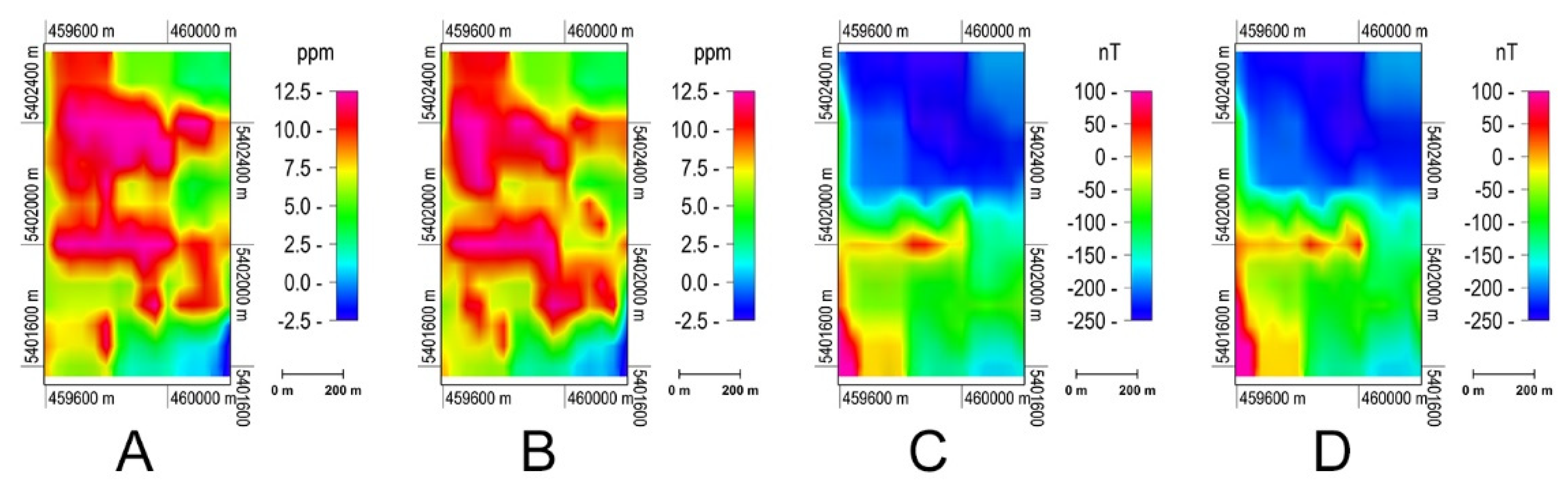
For joint inversion, we selected the frequency domain DIGHEM and total magnetic intensity TMI data collected over a subdomain of the test site.
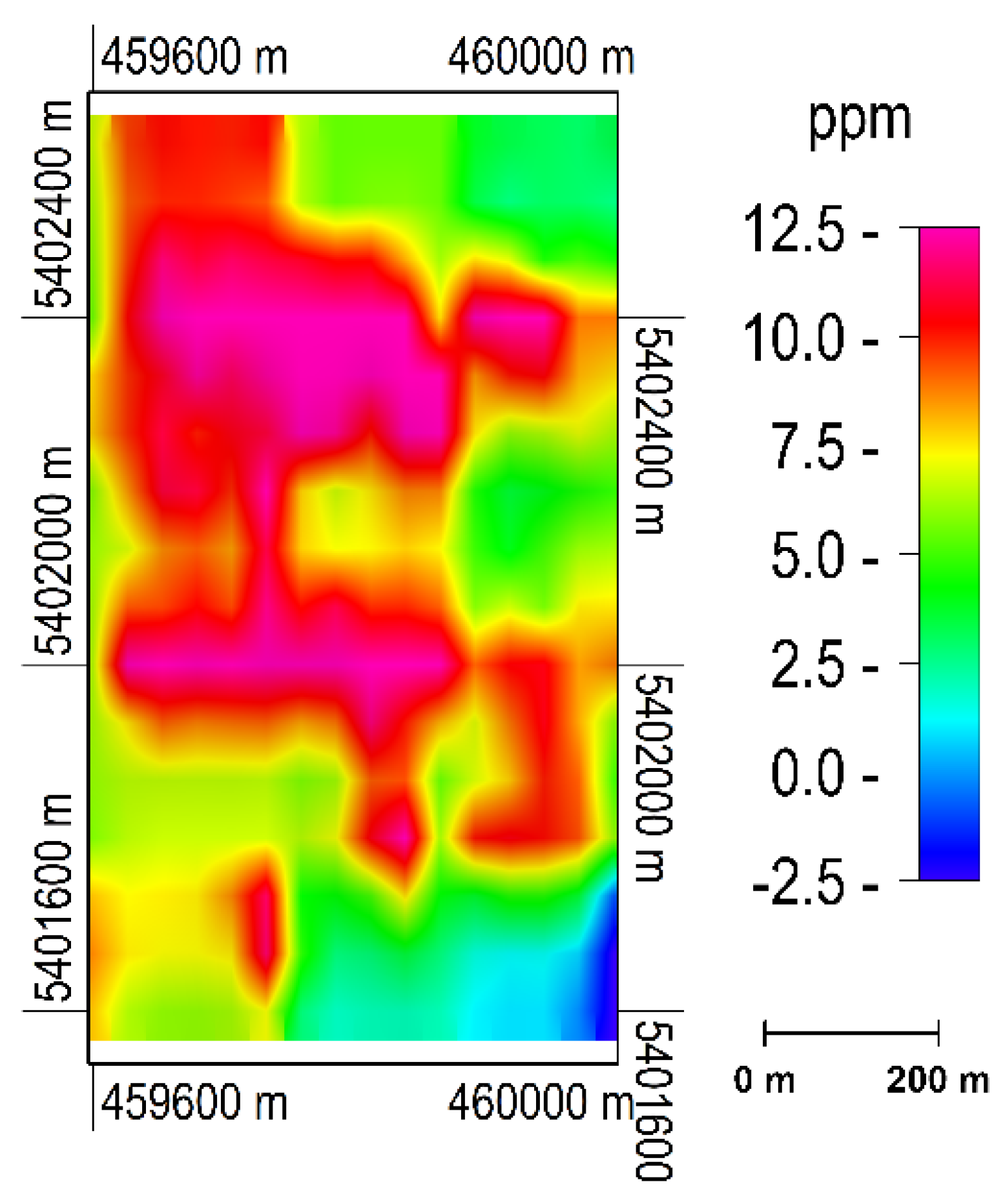
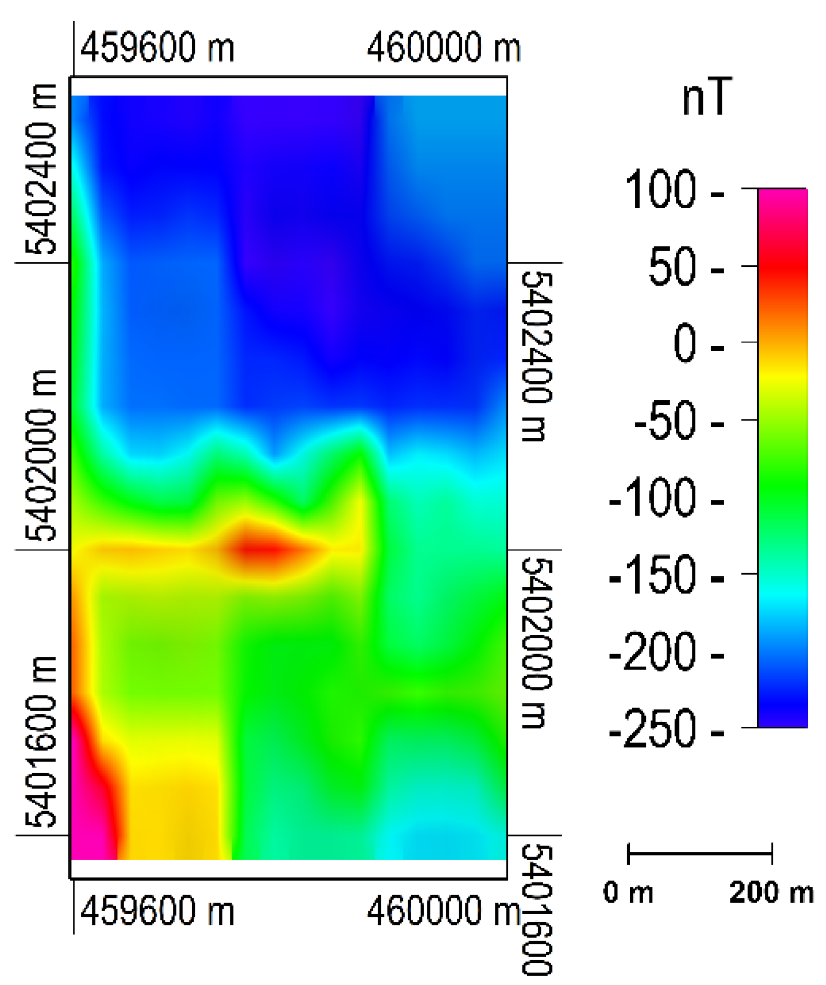
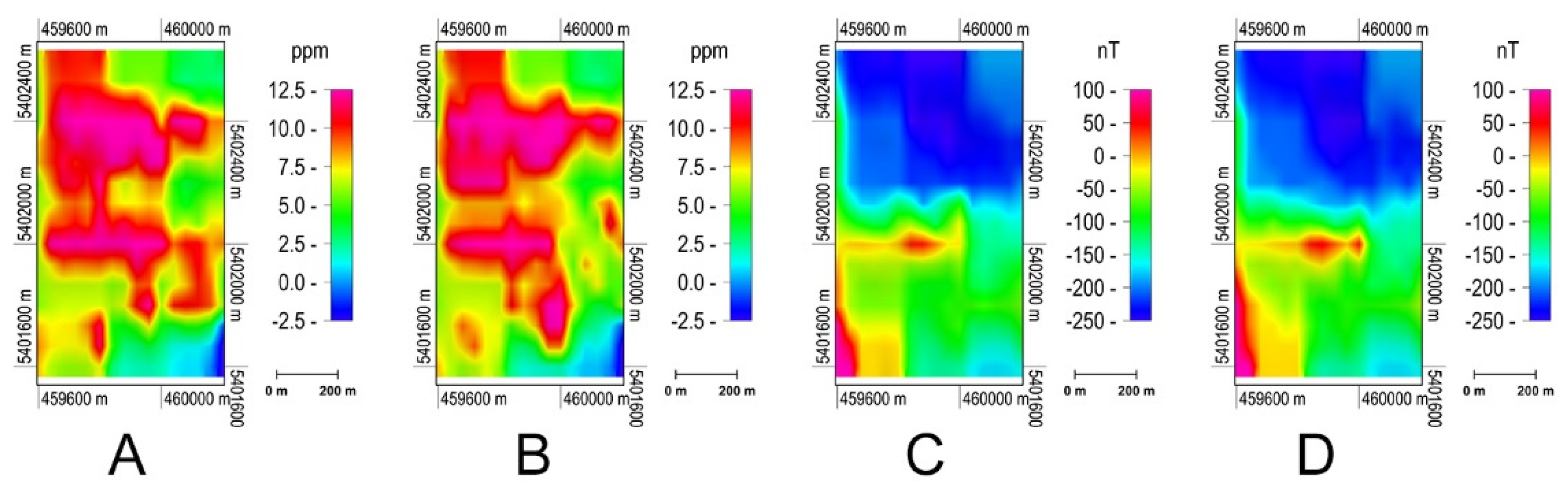
Figure 2 presents a map of 1068 Hz coaxial DIGHEM observed data. The TMI data were filtered by applying the third order polynomial regional trend to emphasize responses from the anomalous sources.
Figure 3 presents the filtered TMI data over the same area.
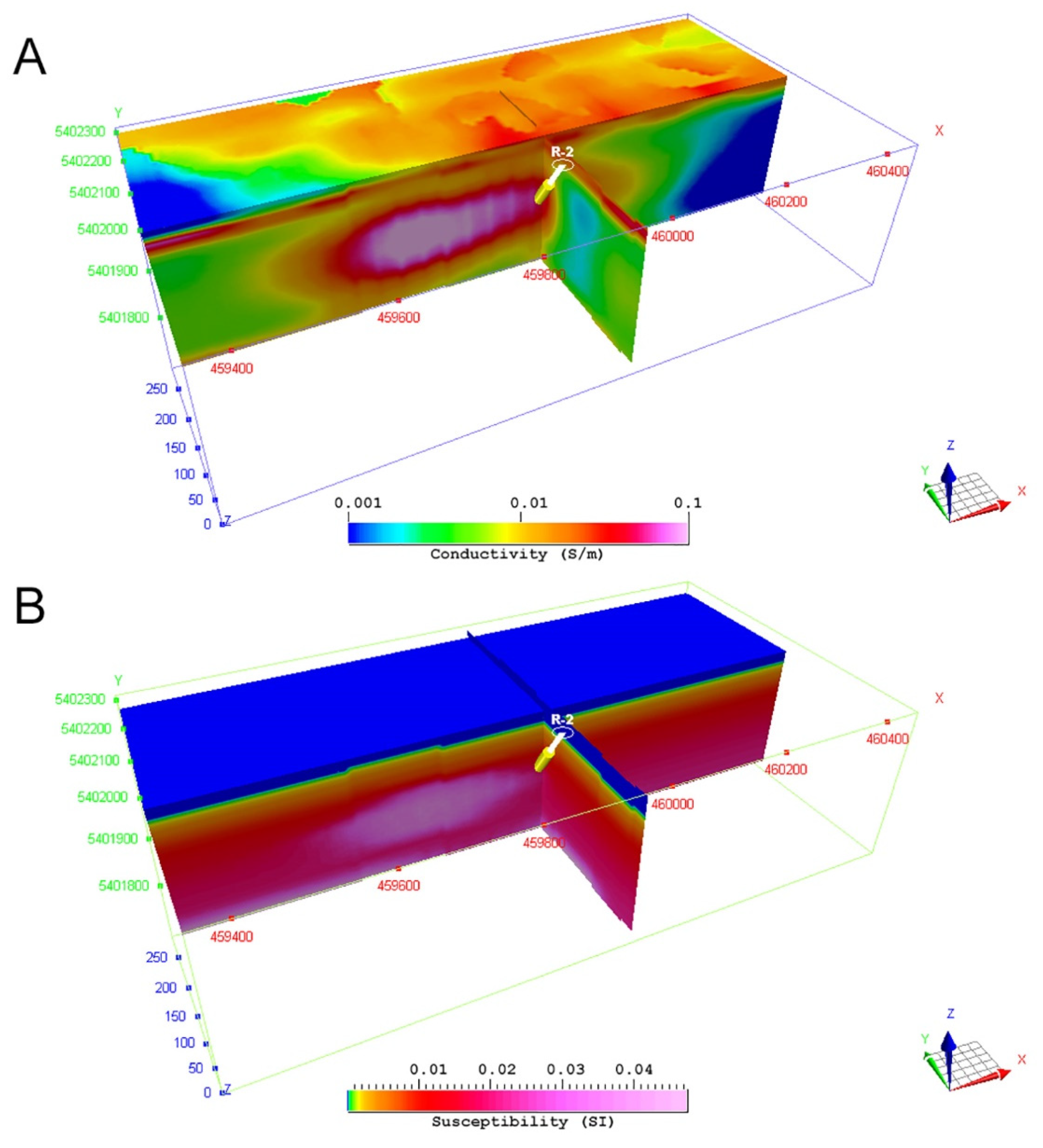
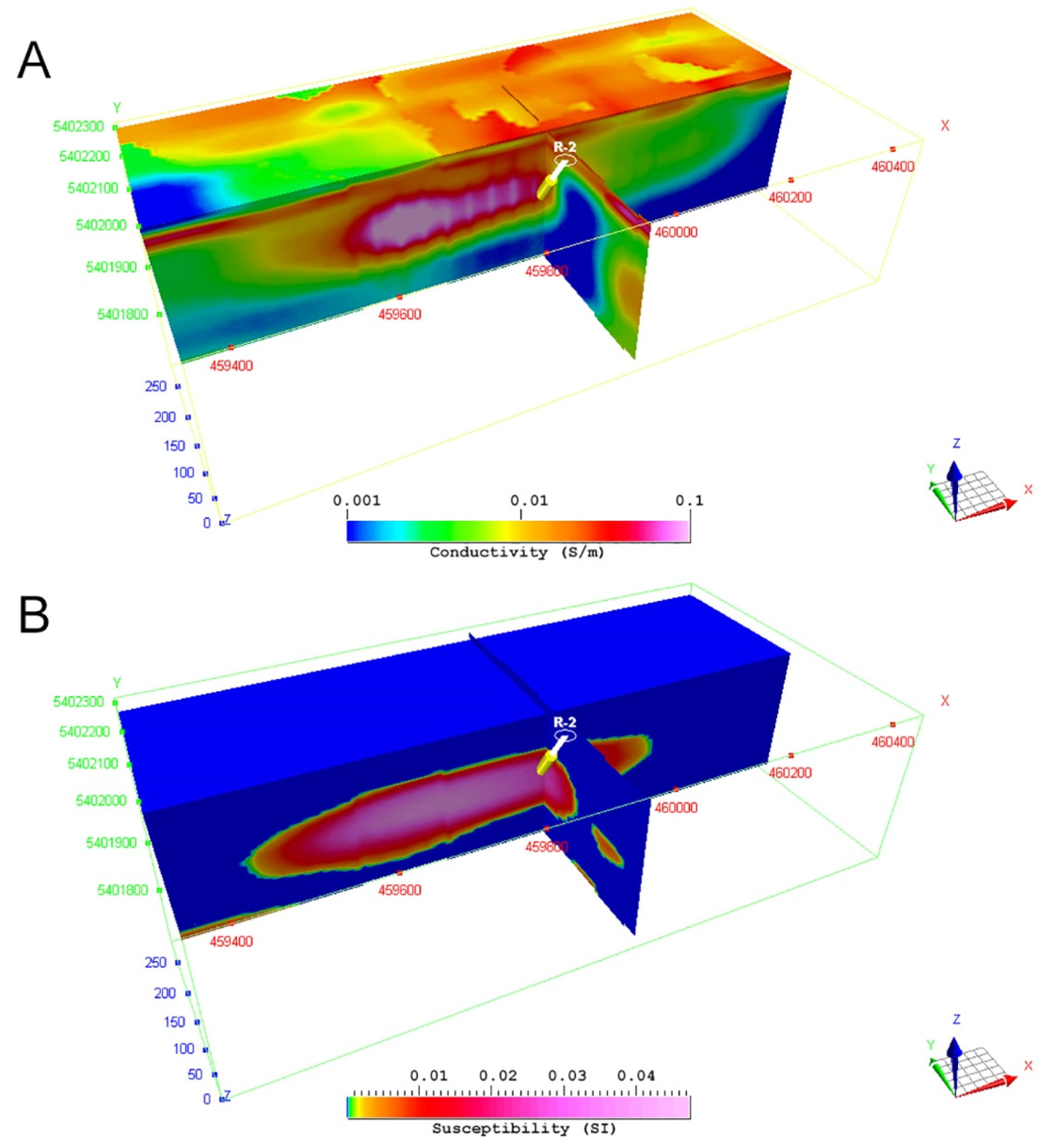
We have applied the standalone inversions to both DIGHEM and TMI data. Panel A in
Figure 4 shows the conductivity model obtained by the standalone inversion. It corresponds well to borehole information [
38] for this target, which indicates conductive overburden to a depth of ≈50 m, underlain by layers of intrusive intermediate and felsic rocks and a strongly fractured graphitic ultramafic intrusion, with concentrations of pyrite and pyrrhotite up to 80% from 100–120 m measured from the surface. Panel B in
Figure 4 presents the magnetic susceptibility model produced by the standalone inversion of the TMI data. This model resolves a layer of intermediate and felsic volcanics at the bottom of the domain, underlying the ultramafic intrusion, which complicates isolation of the ultra-mafic-hosted target.
Figure 5A,B shows the conductivity and susceptibility models produced by joint inversion of DIGHEM and TMI data with Gramian-based structural constraints. These models have similar geospatial boundaries, a high degree of structural correlation, and make isolation of the ultramafic-hosted target much easier.
Figure 6 and
Figure 7 present the observed and predicted data for both inversion approaches. Both methodologies achieve comparable levels of data misfit.
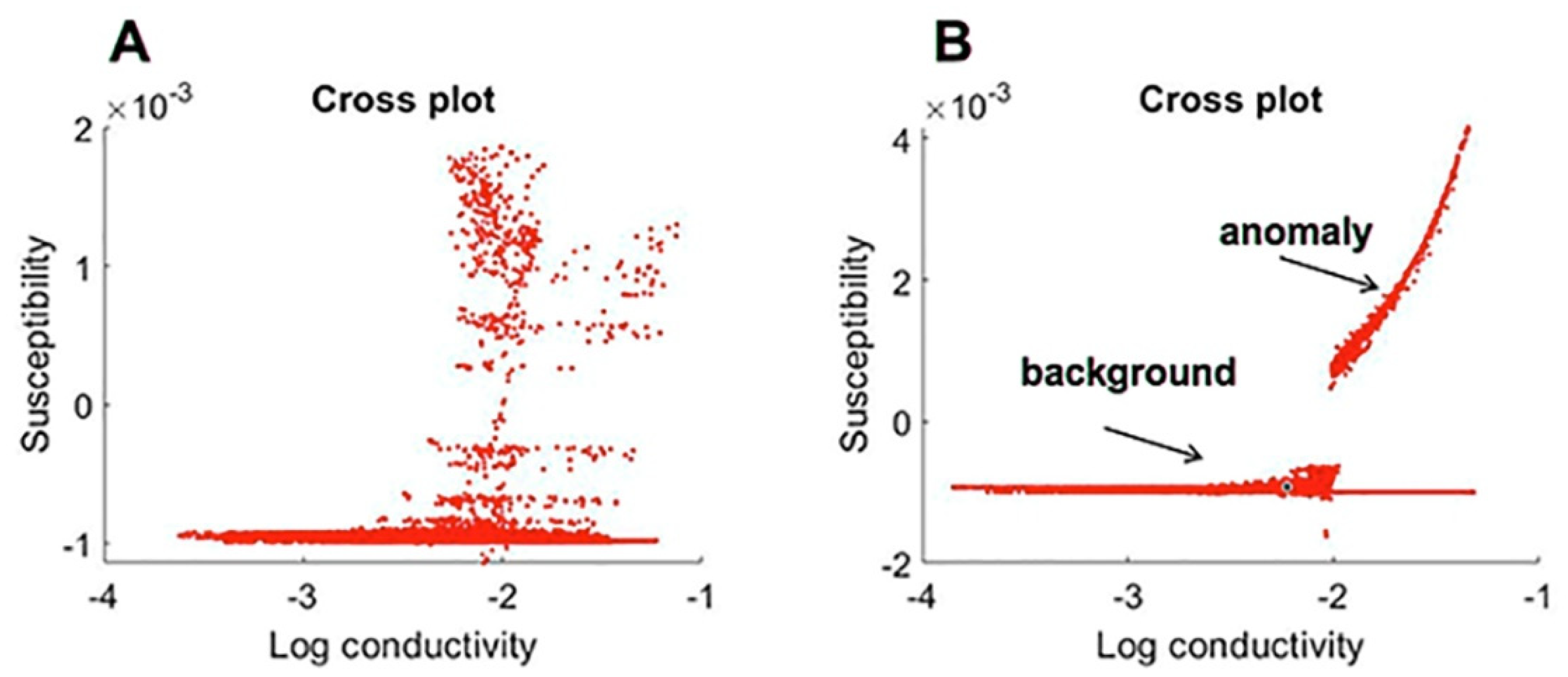
Finally,
Figure 8 shows the cross-correlation plots between susceptibility and log conductivity produced by standalone and joint inversions. The indistinct pattern representing the standalone inverted models in Panel A indicates a minimal structural correlation between the models. In Panel B, conversely, a parabolic trend is apparent. This trend indicates a high degree of structural correlation between the jointly inverted models. Interestingly, we can see two distinct trends in correlations corresponding to background models and the anomalous zone with massive sulfide (VMS) mineralization, respectively.


