Proceeding Paper

Tracking Control for Piezoelectric Actuators with Advanced Feed-Forward Compensation Combined with PI Control †

1
System Engineering and Automation Department, Faculty of Engineering of Vitoria-Gasteiz, Basque Country University (UPV/EHU), 01006 Vitoria-Gasteiz, Spain
2
Fundación Centro de Tecnologías Aeronáuticas (CTA), Juan de la Cierva 1, 01510 Miñano, Spain
*
Authors to whom correspondence should be addressed.
Presented at the First International Electronic Conference on Actuator Technology: Materials, Devices and Applications, 23–27 November 2020; Available online: https://iecat2020.sciforum.net/.
Proceedings 2020, 64(1), 29; https://doi.org/10.3390/IeCAT2020-08481
Published: 20 November 2020

Abstract

:
Piezoelectric Actuators (PEAs) are devices that can support large actuation forces compared to their small size and are widely used in high-precision applications where micro- and nano-positioning are required. Nonetheless, these actuators have undeniable non-linearities, the well-known ones being creep, vibration dynamics, and hysteresis. The latter originate from a combination of mechanical strain and electric field action; as a consequence, these can affect the PEA tracking performance and even reach instability. The scope of this paper is to reduce the hysteresis effect using and comparing different control strategies like feedback with a Feed-Forward (FF) structure, which is often used to compensate the non-linearities and diminish the errors due to uncertainties. In this research, black-box models are analyzed; subsequently, a classic feedback control like Proportional-Integral (PI) control is combined with the FF methods proposed separately and embedded into a dSpace platform to perform real-time experiments. Results are analyzed in-depth in terms of the error, the control signal, and the Integral of the Absolute Error (IAE). It is found that with the proposed methods, the hysteresis effect could be diminished to acceptable ranges for high-precision tracking with a satisfactory control signal.

1. Introduction

PEAs are high-precision positioning systems with a wide range of usage such as active vibration systems for vehicles [1], sensing [2], energy recovery [3], and stick-slip motors [4]. These devices not only are accurate, but also possess a broad stiffness in comparison to their size [5]. Despite the advantages, these actuators have hysteresis, which is a significant non-linearity effect that downgrades the performance. This feature occurs as a combination between the electric field and material and mechanical strain [6], which results in the PEAs having a position-error of up to 22% [7].
Over the years, the hysteresis has been reduced provided that proper control was well designed. Due to the simplicity and robustness, Sliding Mode Control (SMC) is a successful and widely used tool for PEAs [8]; for example, the authors of [9] presented an SMC with a PID-type sliding surface, which was implemented in real-time. In their study, the authors used a PEA with an asymmetrical hysteresis, and they designed the controller based on a state observer with a conventional Bouc–Wen (BW) model (which is inflexible for asymmetry [10]). Even though the accuracy was increased, SMC is naturally known for the chattering effect. Other model-based control strategies could have more accurate models like Prandtl–Ishlinskii or Preisach for state observation, but these are widely complex to implement due to the inverse calculation. For instance, a Prandtl–Ishlinskii model was used in [11], the calculation of which is purely mathematical and lacks practicality.
Authors from [12] suggested that a feedback controller can handle errors in positioning, as well as the reduction of unknown effects; also, the addition of an FF amplifies the nonlinearity compensation. Black-Box (BB) models are commonly used for FF compensation due to the mapping ability for unknown dynamic systems [13], where the common structures are Artificial Neural Networks (ANNs), Hammerstein–Wiener (HW), etc. In [14], a sophisticated FF with feedback control was used: a linear approximation was done, and it was compared with an ANN, which was used for mapping; additionally, a conventional PI and a neural PID were embedded for the whole combination. The outcomes showed that a neural PID with an FF-ANN could improve accuracy. Even though ANNs could give satisfactory results for mapping, other BB strategies could be used. HW is an approach that uses both authors’ theories to identify non-linear dynamic models [15], where the structure consists of non-linear peripheral blocks and a central linear one. An application with an HW was implemented in [16], where the author used the HW block to model the non-linearities of a piezoelectric pad, which was combined with a Kalman filter to estimate the position that was controlled by a fuzzy-PID. The results showed an increment in the accuracy due to the complex structure.
In this research, we use a PI controller whose parameters are optimized by the reduction of the IAE; moreover, an ANN and HW are designed in MATLAB/Simulink, contrasted, and tested individually in a control architecture with a PI. In Section 2, the hardware configuration is explained within the PEA specifications followed by a shallow description of the hysteresis and the control structures used during the experiments. Section 3 provides the results of the hysteresis fitting that the ANN and HW provide; also, the errors and actuation signals are interpreted for the control architectures. Finally, Section 4 provides a summarize of the whole research and which future strategies could be analyzed.

2. Methods

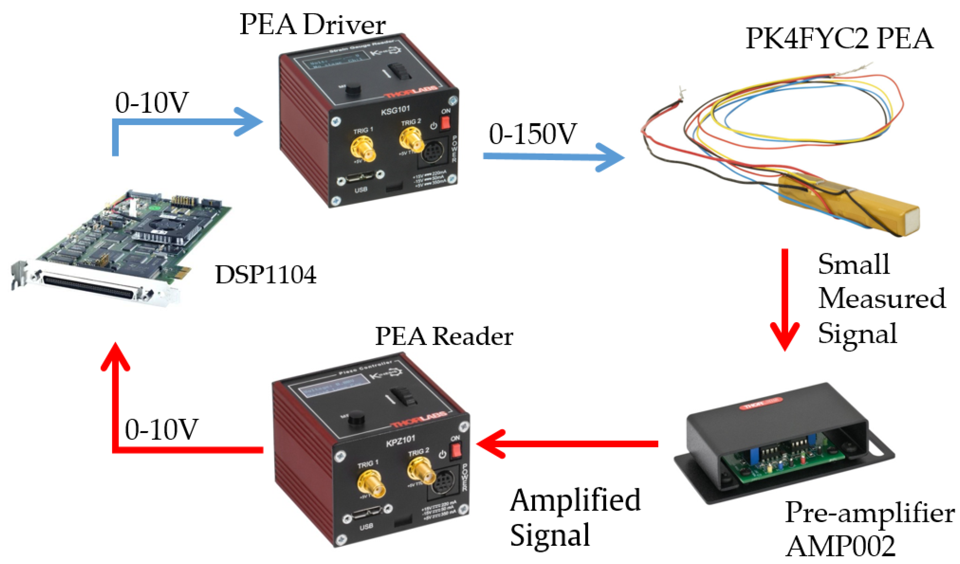
2.1. Hardware Description
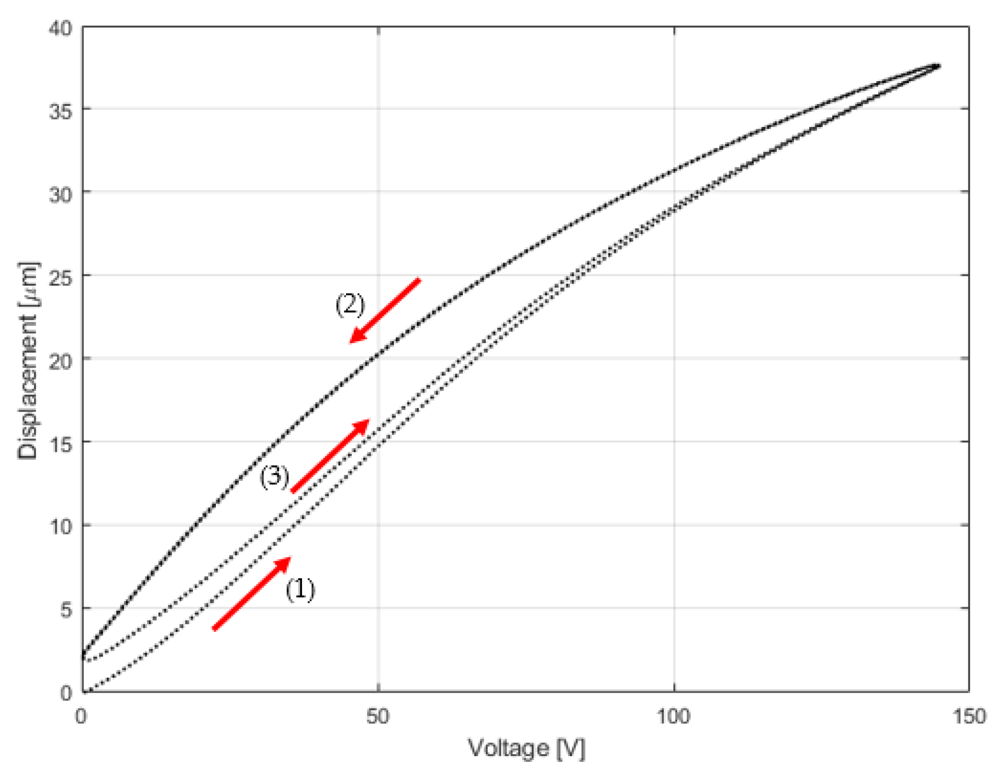
This study was based on commercial hardware from Thorlabs, which was used for the experiments. The PEA PK4FYC2 is a discrete stack actuator where the measurement is done by a full-bridge Wheatstone circuit. A technical description is provided in Table 1.
Figure 1 shows the hardware architectures in which the control strategies were embedded in a dSpace DSP1104 that provided a 0–10 V signal, which is sent to the PEA driver cube (KPZ101 by Thorlabs); this hardware amplifies the signal of 0–150 V straight into the PEA. The measurement is done in two steps: the strain gauge measurement is augmented in a pre-amplifier AMP002 and linked to a strain gauge reader KPZ101 by Thorlabs. The latter provides a 0–10 V measurement signal, which is used in the DSP1104 hardware for control purposes.

2.2. PEA Hysteresis

The hysteresis was obtained through a triangle wave as the input voltage; also, mathematically, it represents the sum of infinite harmonics, which implies that any proposed controller needs to grant high performance to tracking [17]. According to [14], the PEA used reflects a prominent hysteresis effect at the maximum driving voltage, so for the tests and to avoid damage, it was configured at 145 V, and the period was set at 1 second. The sampling time was configured at 1 kHz, which reflects a suitable balance between acquisition and hardware limitation.
Figure 2 is the PK4FY2 PEA hysteresis graph for two cycles at the start. Usually, the hysteresis tends to converge the loop between (2) and (3) since the position only begins at zero whenever calibration is done before any operation.

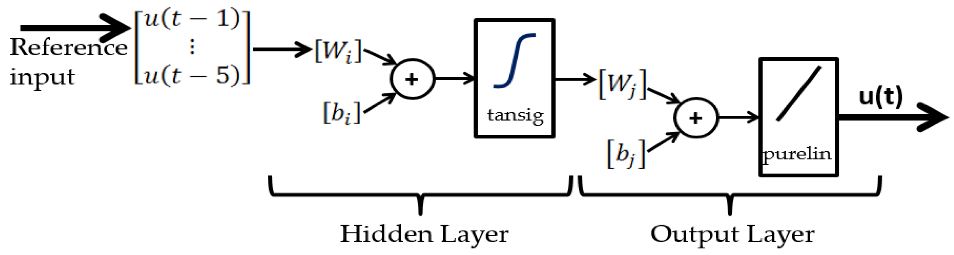
2.3. ANN Configuration

The first architecture used for mapping the PEA non-linearity was a Time Delay Neural Network (TDNN), which is a recurrent ANN [18] type. The structure implies that the predicted output depends on the past values of the input (which was set as 5 by default) and merged with a non-linear function f, as shown in Equation (1). The function f was approximated by a non-linear combination of a hidden and output layer with its activation functions and weights. Figure 3 displays the architecture of the TDNN where both layers have different weights and biases (in terms of i and j). The configuration of the ANN was disposed as the one used by the author in [14] where the number of neurons in the hidden layer was 22. The training information was set as 10 seconds of triangle waves, which reflected the PEA displacement and voltage as the input and output, respectively. Furthermore, the data were divided into 70% for training, 15% for validation, and the rest for testing. The training algorithm used was Levenberg–Marquardt (LM) as the MATLAB ANN Toolbox suggests; the calculation was carried until acceptable values of the Mean Squared Error (MSE) were achieved.
y ( t ) = f ( u ( t 1 ) , , u ( t 5 ) )

2.4. Hammerstein–Wiener Configuration

As Figure 4 shows, HW consists of three blocks in series where the outer ones are used to map the input and output non-linearities, whereas the middle block is a linear function (Equation (2)) in terms of the time shift operator q 1 , such that q 1 u ( t ) = u ( t T ) . The parameters n b , n f , and n d represent the degree of B, F, and the delay, respectively.
B F = q n d i = 1 n b b i q i + 1 1 + j = 1 n f b j q j
The parameters of the HW block were estimated with the MATLAB System Identification Toolbox, which uses a loss function based on the error reduction between the model output and the measured response as a metric. The approximation algorithm was set to the automatic choice according to the toolbox criterion. The non-linear blocks can be estimated with different functions (such as piece-wise functions, polynomial, wavelet, etc) where the criterion used to determine which could suit it best was the fit percent, which defines the quality of the model likeness to the measured data.

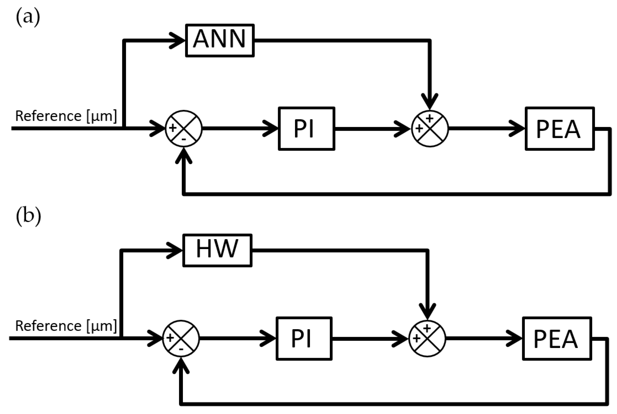
2.5. Control Structure

The experiments were done with two control structures that had the same PI, but with an FF-ANN and an FF-HW (Figure 5). The PI tuning was based on the IAE (Equation (3)) in real time and aiming to reach the best performance. For a fair comparison, the constants K p and K i were the same in both architectures.
I A E = 0 | e ( t ) | d t

3. Results and Discussion

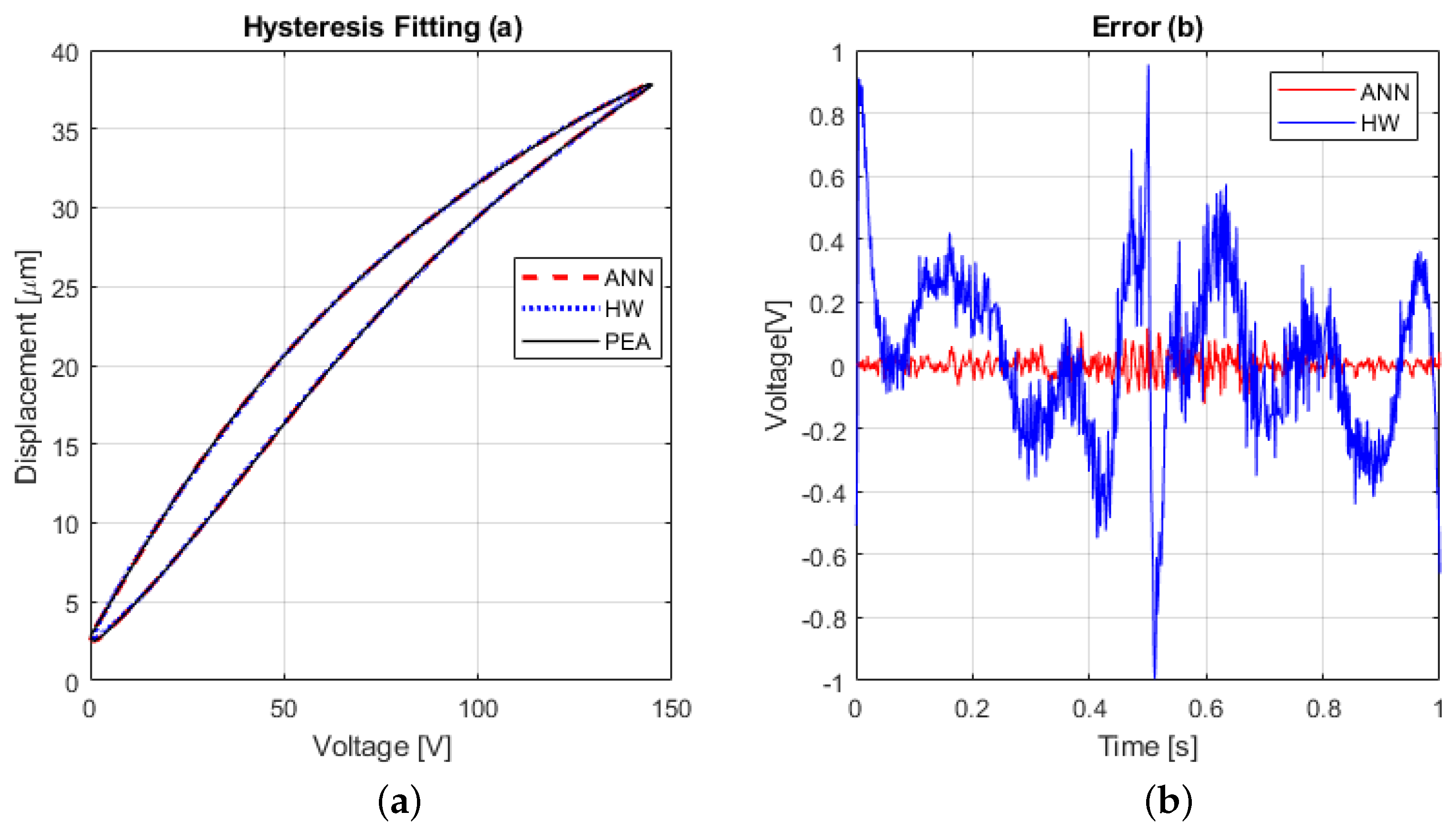
3.1. Hysteresis Fitting Results

Before testing the control structures, the accuracy of each FF block was tested and contrasted. The ANN provided a satisfactory MSE during the training; the HW fitting architecture chosen was a sixth-degree polynomial input-output (Equation (4)) to represent the non-linearities since it contributes the best fit percent in comparison with the other methods.
F ( x ) = c ( 1 ) x n + c ( 1 ) x n 1 + + c ( n ) x + c ( n + 1 )
Figure 6a shows the hysteresis graph with the interpolation of the ANN and HW, which overlap, and for that reason, Figure 6b displays the error in terms of voltage so that the comparison can be appreciated. The ANN behaves significantly better than HW, which has enough distortion. At the peak moment (which occurs at 0.5 s), HW has a sudden behavior that resembles a sign change; this is expected due to the radical change of slope at the peaks. On the other side, the ANN could manage to fit the hysteresis with only a slight noise during the peak, but it can be seen that the error stands on average around the null value.

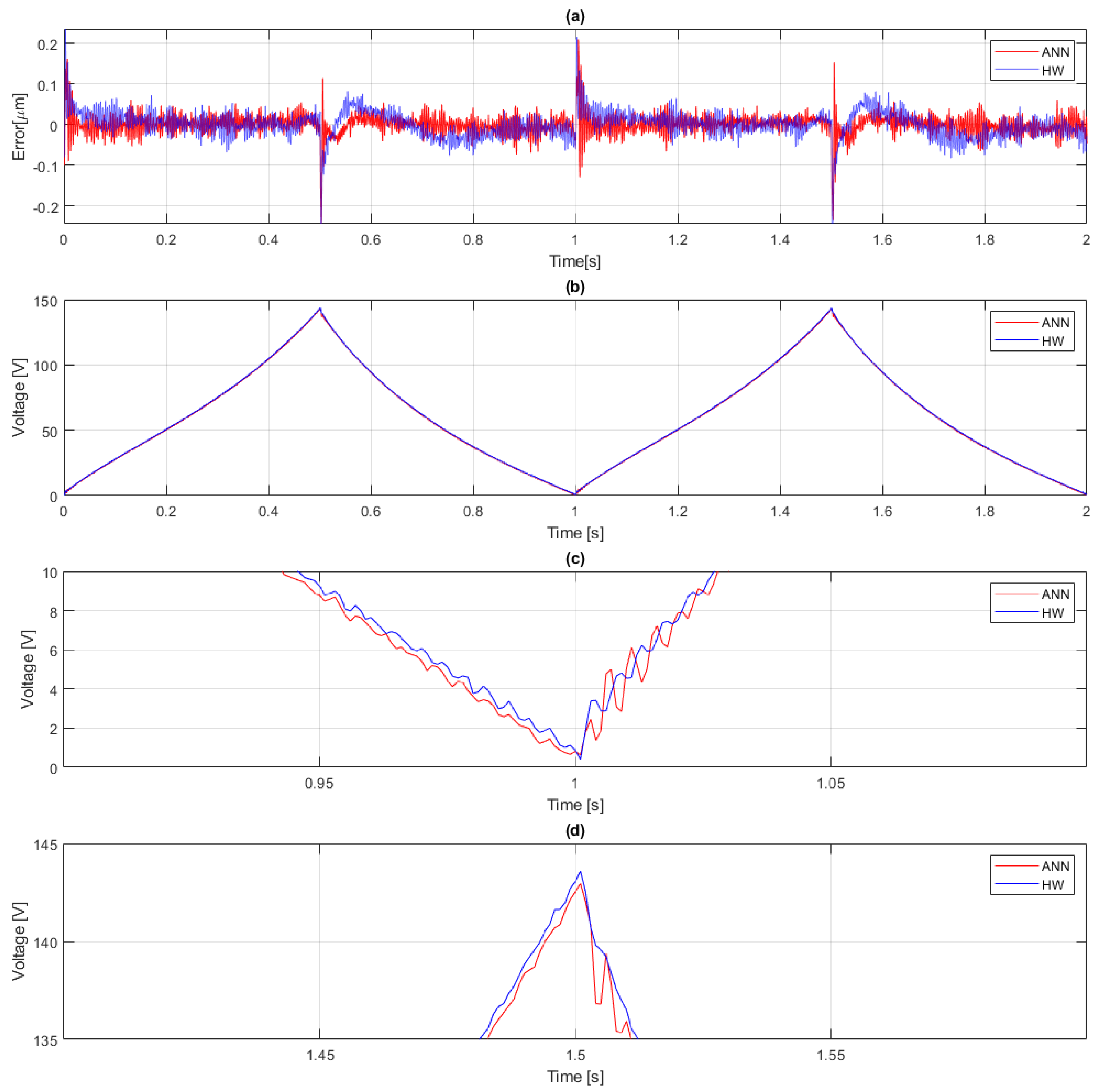
3.2. Guidance Control Results

Despite that HW provided a low-grade hysteresis fit, an objective contrast needs to be made with a control loop so that the control signal can be a metric as well. The PI parameters were tuned to K p and K i equal to 10 and 100, respectively. The IAE showed values of 0.0384 and 0.0486, which belong to the FF-ANN and FF-HW (both with PI control), respectively. This resembles the difference being 26% higher when the ANN was used; however, the in-depth analysis is presented in the following section.
Figure 7a is the error contrast between the models: the control loop with the FF-HW resulted in less accurate results where the main differences could be seen in special places of the graph. During the first rise, both models managed to behave with a modest difference, but at the first peak where the slope shifts, a soaring error increment for FF-HW was provoked. During the decline, the framework with FF-HW compensated the error faster, although it had more overshoot and a later undulation. The lower peak at one second behaved reciprocally for both models where the one compensated with the ANN had more noise.
Although the control signal from Figure 7b looks similar in both cases, Figure 7c,d displays an amplified view during both peaks. Even if the FF-HW model was less accurate, during the control signal, it showed an improvement since the variation was less than the FF-ANN. During the rise, the control signal of the framework with HW had a lower amplitude compared to the ANN , and the same happened after the descent.

4. Conclusions

In this research, we analyze different mapping alternatives to be used in a feedback FF control architecture. It is found that the hysteresis is an undesirable effect and complex to model with conventional tools due to the asymmetry (which was present in the PEA used), and thus, alternative solutions such as a BB can deal with this problem.
The PEA hysteresis is obtained with a triangle wave, which is a complex signal and implies that the control design has to be robust enough. Therefore, a comparison between HW and the ANN is done to verify the mapping accuracy. HW shows low performance in comparison with the ANN since the error has more fluctuation and could carry the peak with certain difficulties. The ANN has an increment in the accuracy that is near the null value of error on average.
However, the control tests show a different situation, since the architecture with the FF-HW has an advantage compared to the FF-ANN. The latter achieves a lower error (which is reflected in the IAE) and performs better than the FF-HW. However, the one with FF-HW shows that the control signal is superior: the signal has less undulation and is smoother as well. This implies that the actuation effort is less, so that the life-span of the PEA could increase even though the accuracy is lower. Therefore, with this research, the designer has two options to choose, which have pros and cons depending on the requirements.
Regarding the options for future research, several combinations can be made. For instance, the PI controller can be replaced with a Fractional-Proportional-Derivative-Integral (FPID) so that the complexity is higher. Another option is the usage of a neural PID with advance learning rules. In terms of the FF block, different ANN architectures can be used like Long-Short-Term Memory (LSTM); also an optimization of the HW block can be done by a study using a Hammerstein or a Wiener block so that the calculation is reduced, as well as the complexity.

Author Contributions

Conceptualization, O.B. and C.N.; methodology, O.B., I.C., and C.N.; software, C.N.; validation, C.N.; formal analysis, O.B. and C.N.; investigation, O.B. and C.N.; resources, C.N.; writing, original draft preparation, C.N. and M.D.; writing, review and editing, O.B., C.N., M.D., and M.Y.S.; supervision, O.B. and I.C.; project administration, O.B. and J.V. All authors read and agreed to the published version of the manuscript.

Funding

This research was funded by the Basque Government and the UPV/EHU projects.

Acknowledgments

The authors wish to express their gratitude to the Basque Government through the project SMAR3NAK (ELKARTEK KK-2019/00051), to the Diputación Foral de Álava (DFA) through the project CONAVAUTIN 2, and to the UPV/EHU for supporting this work.

Conflicts of Interest

The authors declare no conflict of interest.

Abbreviations

The following abbreviations are used in this manuscript:
PEAPiezoelectric Actuator
FFFeed-Forward
PIProportional-Integral
IAEIntegral of the Absolute Error
SMCSliding Mode Control
BWBouc–Wen
BBBlack-box
ANNArtificial Neural Networks
HWHammerstein–Wiener
TDNNTime Delay Neural Network
LMLevenberg–Marquardt
MSEMean Squared Error

References

  1. Gäbel, G.; Millitzer, J.; Atzrodt, H.; Herold, S.; Mohr, A. Development and Implementation of a Multi-Channel Active Control System for the Reduction of Road Induced Vehicle Interior Noise. Actuators 2018, 7, 52. [Google Scholar] [CrossRef]
  2. Toledo, J.; Ruiz-Díez, V.; Hernando-García, J.; Sánchez-Rojas, J.L. Piezoelectric Actuators for Tactile and Elasticity Sensing. Actuators 2020, 9, 21. [Google Scholar] [CrossRef]
  3. Ai, R.; Monteiro, L.L.S.; Monteiro, P.C.C., Jr.; Pacheco, P.M.C.L.; Savi, M.A. Piezoelectric Vibration-Based Energy Harvesting Enhancement Exploiting Nonsmoothness. Actuators 2019, 8, 25. [Google Scholar] [CrossRef]
  4. Hunstig, M. Piezoelectric Inertia Motors—A Critical Review of History, Concepts, Design, Applications, and Perspectives. Actuators 2017, 6, 7. [Google Scholar] [CrossRef]
  5. Huang, Y.; Xia, Y.X.; Lin, D.H.; Lim, L.-C. High-Bending-Stiffness Connector (HBSC) and High-Authority Piezoelectric Actuator (HAPA) Made of Such. Actuators 2018, 7, 61. [Google Scholar] [CrossRef]
  6. Bertotti, G.; Mayergoyz, I.; Damjanoivc, D. Hysteresis in Piezoelectric and Ferroelectric Materials. In The Science of Hysteresis; Elsevier: Riverport Lane, MD, USA, 2006; Volume 3, pp. 338–448. [Google Scholar]
  7. Frederik, F.; Minorowicz, N. Open loop control of piezoelectric tube transducer. Mech. Technol. Mater. 2018, 38, 23–28. [Google Scholar]
  8. Velasco, J.; Barambones, O.; Calvo, I.; Zubia, J.; Ocariz, I.; Chouza, A. Sliding Mode Control with Dynamical Correction for Time-Delay Piezoelectric Actuactor Systems. Materials 2019, 13, 132. [Google Scholar] [CrossRef] [PubMed]
  9. Chouza, A.; Barambones, O.; Calvo, I.; Velasco, J. Sliding Mode-Based Robust Control for Piezoelectric Actuators with Inverse Dynamics Estimation. Energies 2019, 12, 943. [Google Scholar] [CrossRef]
  10. Song, J.; Der Kiureghian, A. Generalized Bouc–Wen Model for Highly Asymmetric Hysteresis. J. Eng. Mech. 2006, 132, 610–618. [Google Scholar] [CrossRef]
  11. Tan, X.; Iyer, R.; Krishnaprasad, P.S. Control of hysteresis: Theory and experimental results. Proc. SPIE 2001, 4326, 101–112. [Google Scholar]
  12. Peng, J.; Chen, J. A Survey of Modeling and Control of Piezoelectric Actuators. Mod. Mech. Eng. 2013, 3, 1–20. [Google Scholar] [CrossRef]
  13. Sjöberg, J.; Zhang, Q.; Ljung, L.; Benveniste, A.; Delyon, B.; Glorennec, P.; Hjalmarsson, H.; Juditsky, A. Nonlinear black-box modeling in system identification: A unified overview. Automatica 1995, 31, 1691–1724. [Google Scholar] [CrossRef]
  14. Napole, C.; Barambones, O.; Calvo, I.; Velasco, J. Feedforward Compensation Analysis of Piezoelectric Actuators Using Artificial Neural Networks with Conventional PID Controller and Single-Neuron PID Based on Hebb Learning Rules. Energies 2020, 13, 3929. [Google Scholar] [CrossRef]
  15. Wills, A.; Schön, T.; Ljung, L.; Ninness, B. Identification of Hammerstein–Wiener Models. Automatica 2012, 49, 70–81. [Google Scholar] [CrossRef]
  16. Wang, Y.; Ho, J.; Jiang, Y. A self-positioning linear actuator based on a piezoelectric slab with multiple pads. Mech. Syst. Signal Process. 2021, 150, 107245. [Google Scholar] [CrossRef]
  17. Qin, Y.; Duan, H. Single-Neuron Adaptive Hysteresis Compensation of Piezoelectric Actuator Based on Hebb Learning Rules. Micromachines 2020, 11, 84. [Google Scholar] [CrossRef] [PubMed]
  18. Waibel, A.; Hanazana, T.; Hinton, G.; Shikano, K.; Lang, K.J. Phoneme recognition using time delay neural networks. IEEE Trans. Acoust. Speech Signal Process 1989, 37, 328–339. [Google Scholar] [CrossRef]
Figure 1. Hardware architecture.
Proceedings 64 00029 g001
Figure 2. Piezoelectric hysteresis graph.
Proceedings 64 00029 g002
Figure 3. TDNN explicit architecture.
Proceedings 64 00029 g003
Figure 4. HW architecture.
Proceedings 64 00029 g004
Figure 5. Control architectures where (a) uses an FF-ANN and (b) an FF-HW.
Proceedings 64 00029 g005
Figure 6. Hysteresis fitting accuracy where (a) corresponds to both models in the fitting and (b) is the error for both models.
Proceedings 64 00029 g006
Figure 7. Error comparison and control signal architectures with PI combined with FF-ANN and FF-HW. (a) Error; (b) control signal; (c) control signal at the lower peak; (d) control signal at the top peak.
Proceedings 64 00029 g007
Table 1. Thorlabs PK4FYC2 technical specifications.
PropertiesValuesUnits
Physical dimensions7.3 × 7.3 × 36mm
Nominal max displacement38.5 μ m
Max force1000N
Drive voltage range0–150V
Error due to hysteresis15%
Publisher’s Note: MDPI stays neutral with regard to jurisdictional claims in published maps and institutional affiliations.

