Prediction of Wind Speed Using Hybrid Techniques

 , ,
, ,
Abstract
1. Introduction
- Least-squares support vector machine (LSSVM)
- Empirical mode decomposition (EMD)
- Wavelet transform (WT)
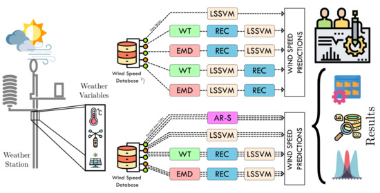
2. Materials and Methods: Wind Speed Prediction
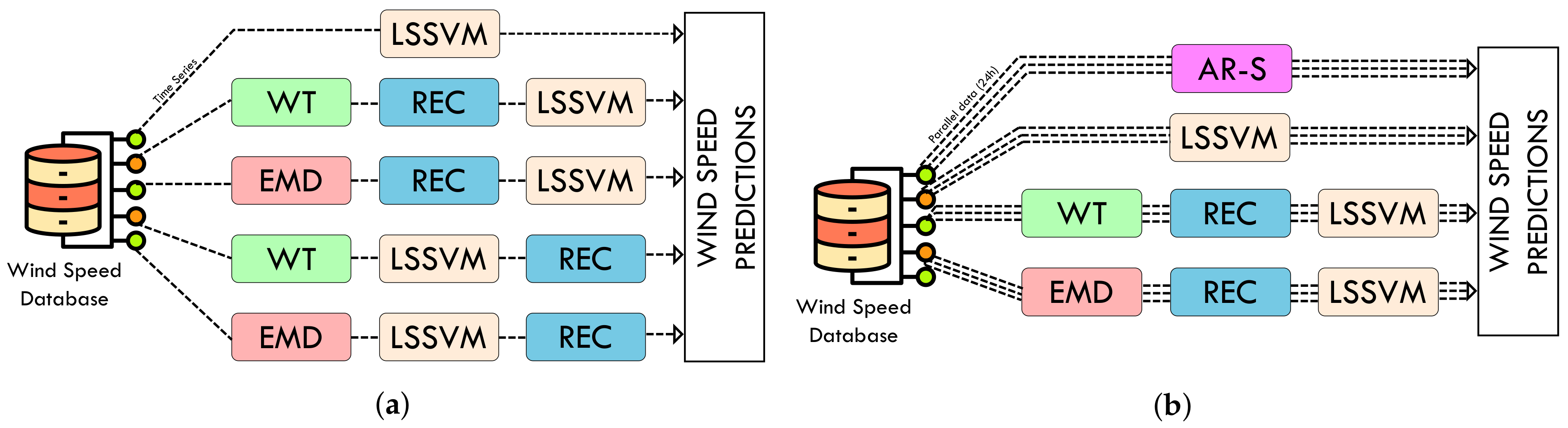
- Method I (series prediction): SER-LSSVM.
- Method II (series prediction): EMD with WT, elimination of high variability component, signal reconstruction (REC) and then use of LSSVM (SER-WT-REC-LSSVM).
- Method III (series prediction): EMD, elimination of high variability component, signal reconstruction and then use of LSSVM (SER-EMD-REC-LSSVM).
- Method IV (series prediction): Decomposition with WT, elimination of high variability component, use of LSSVM to estimate each WT component and then signal reconstruction. (SER-WT-LSSVM-REC).
- Method V (series prediction): EMD, elimination of high variability component, use of LSSVM to estimate each EMD component and then signal reconstruction (SER-EMD-LSSVM-REC).
- Method VI (parallel prediction): Autoregressive model that estimates the wind in one hour using the simple average of the wind at that same time for previous days (PAR-AVE).
- Method VII (parallel prediction): LSSVM at hourly winds for several days (PAR-LSSVM).
- Method VIII (parallel prediction): Decomposition with WT at hourly winds for several days, eliminating the high variability component and then signal reconstruction. Subsequently, LSSVM is used to estimate winds in each of the 24 h (PAR-WT-REC-LSSVM).
- Method IX (parallel prediction): EMD at hourly winds for several days, elimination of the high variability component and then signal reconstruction. Subsequently, LSSVM is used to estimate winds in each of the 24 h (PAR-EMD-REC-LSSVM).
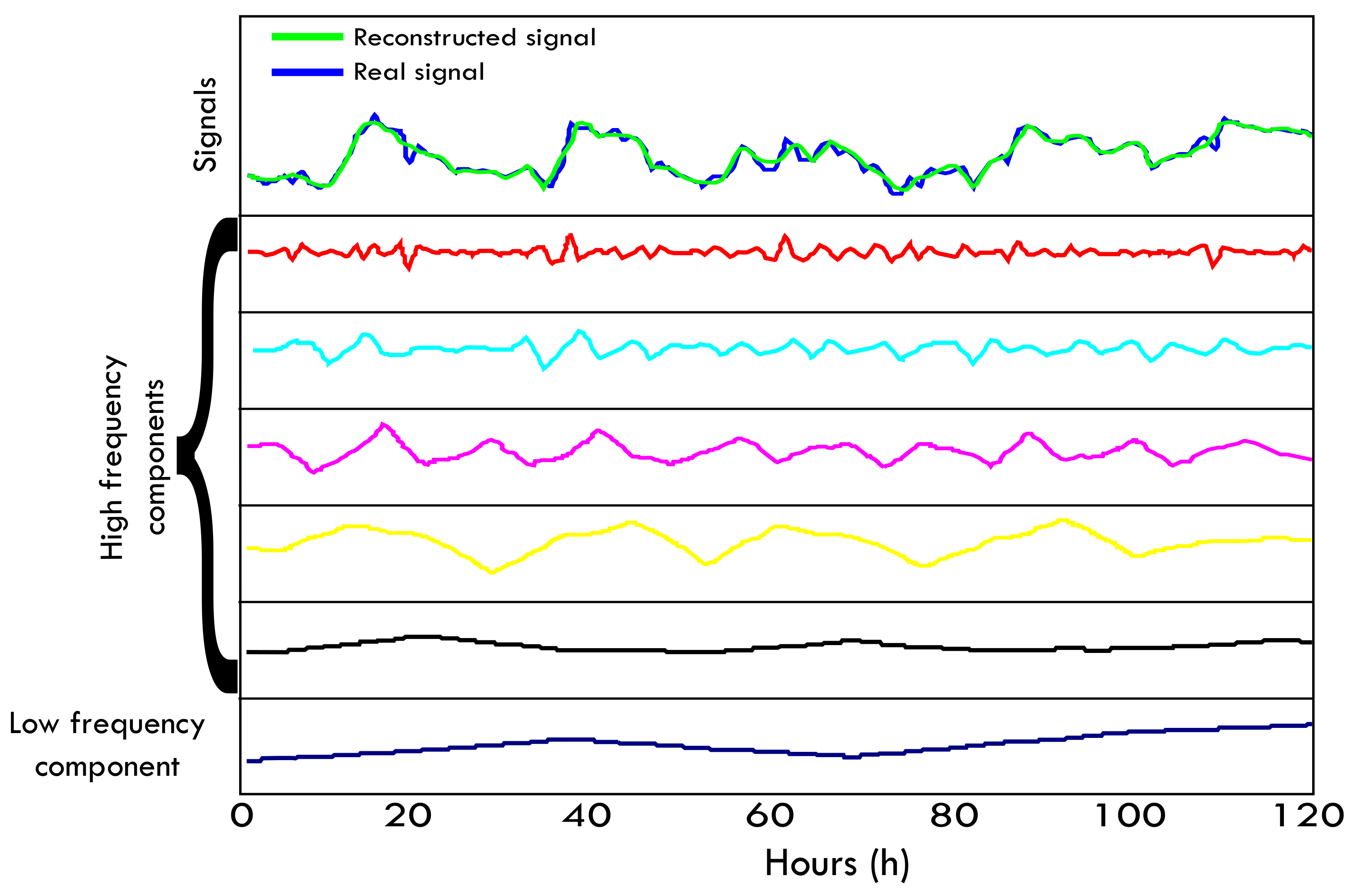
2.1. Wavelet Transform (WT)
2.2. Empirical Mode Decomposition (EMD)
2.3. Least Square Support Vector Machine (LSSVM)
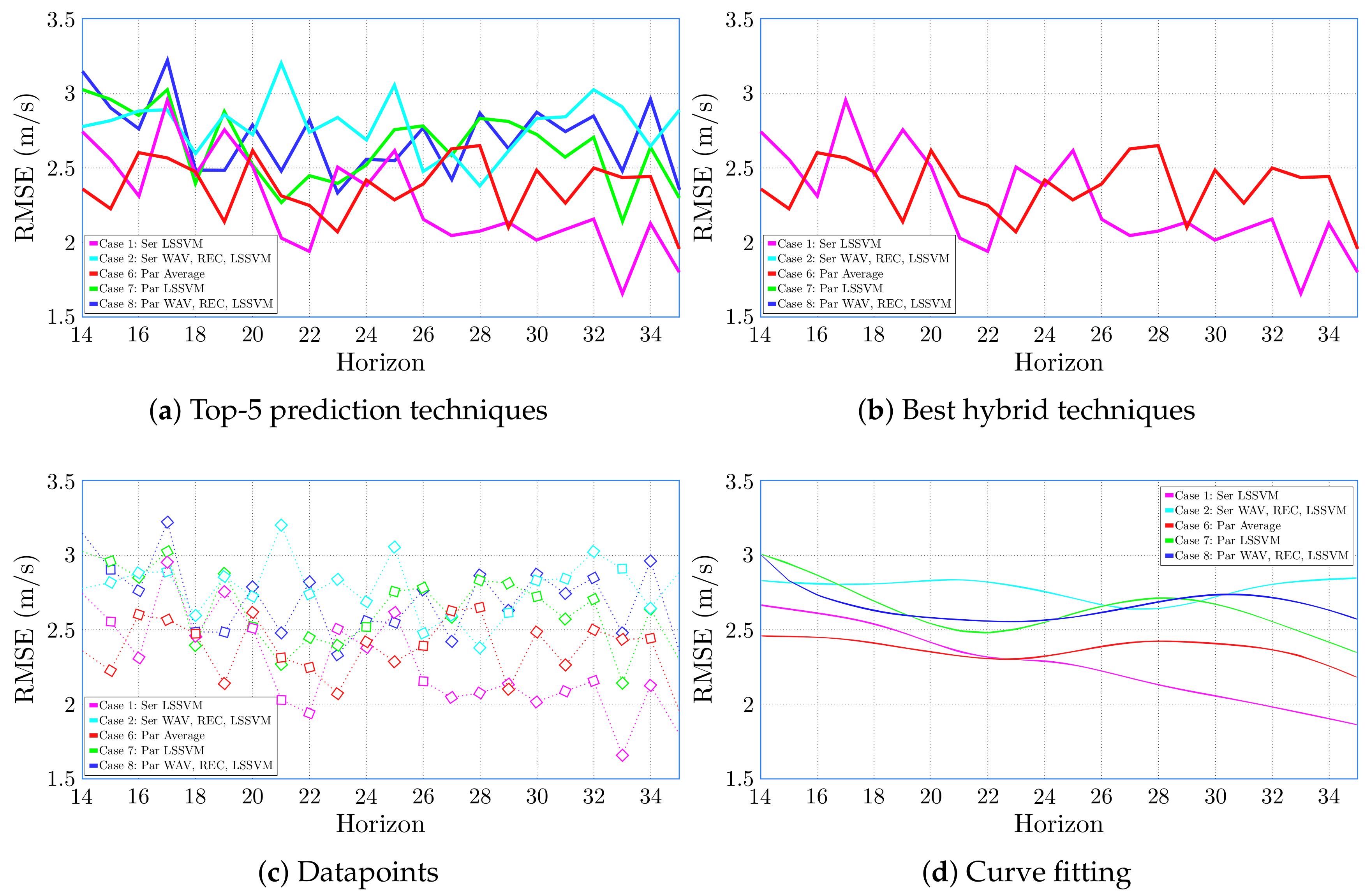
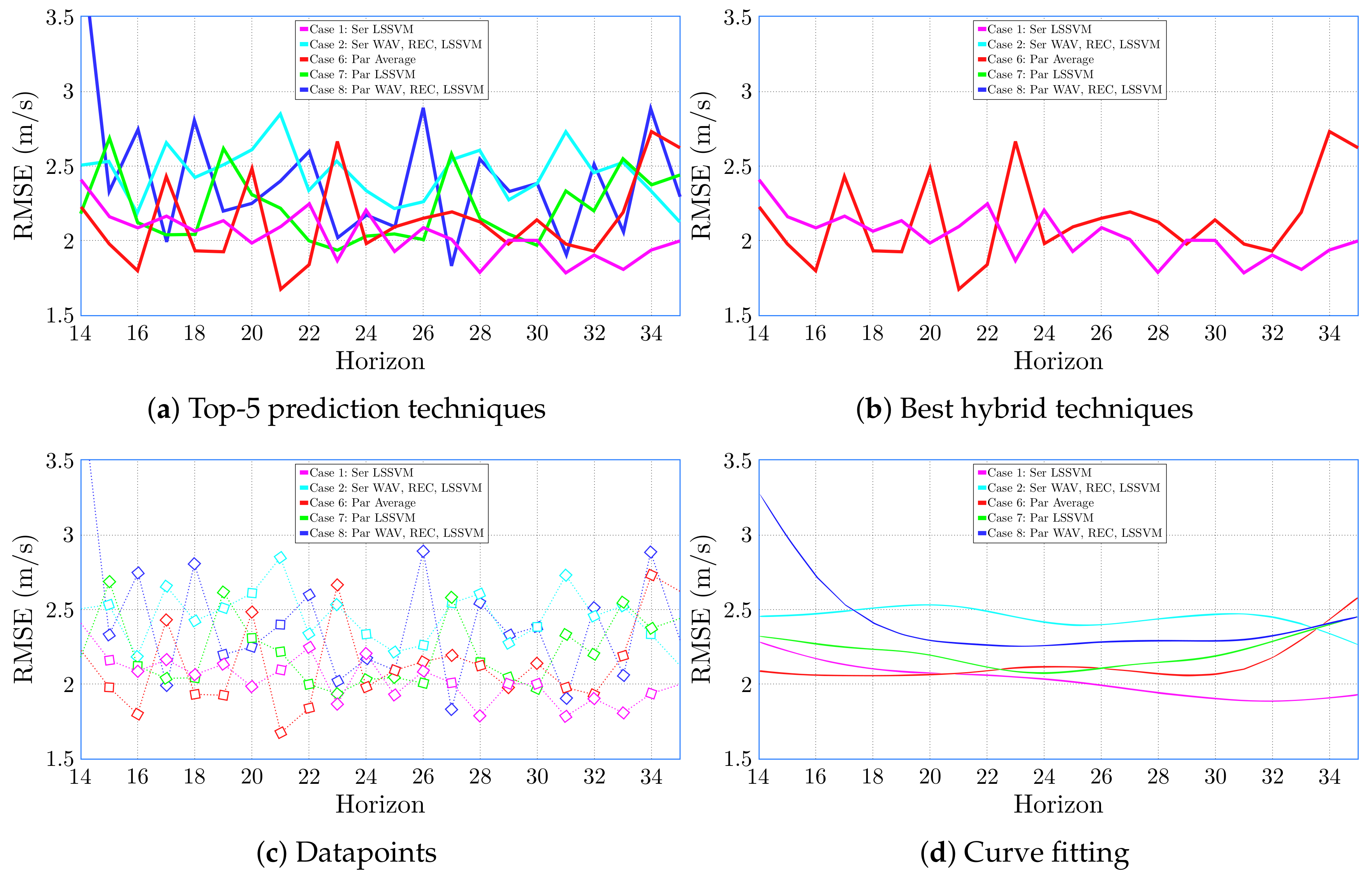
3. Test and Results
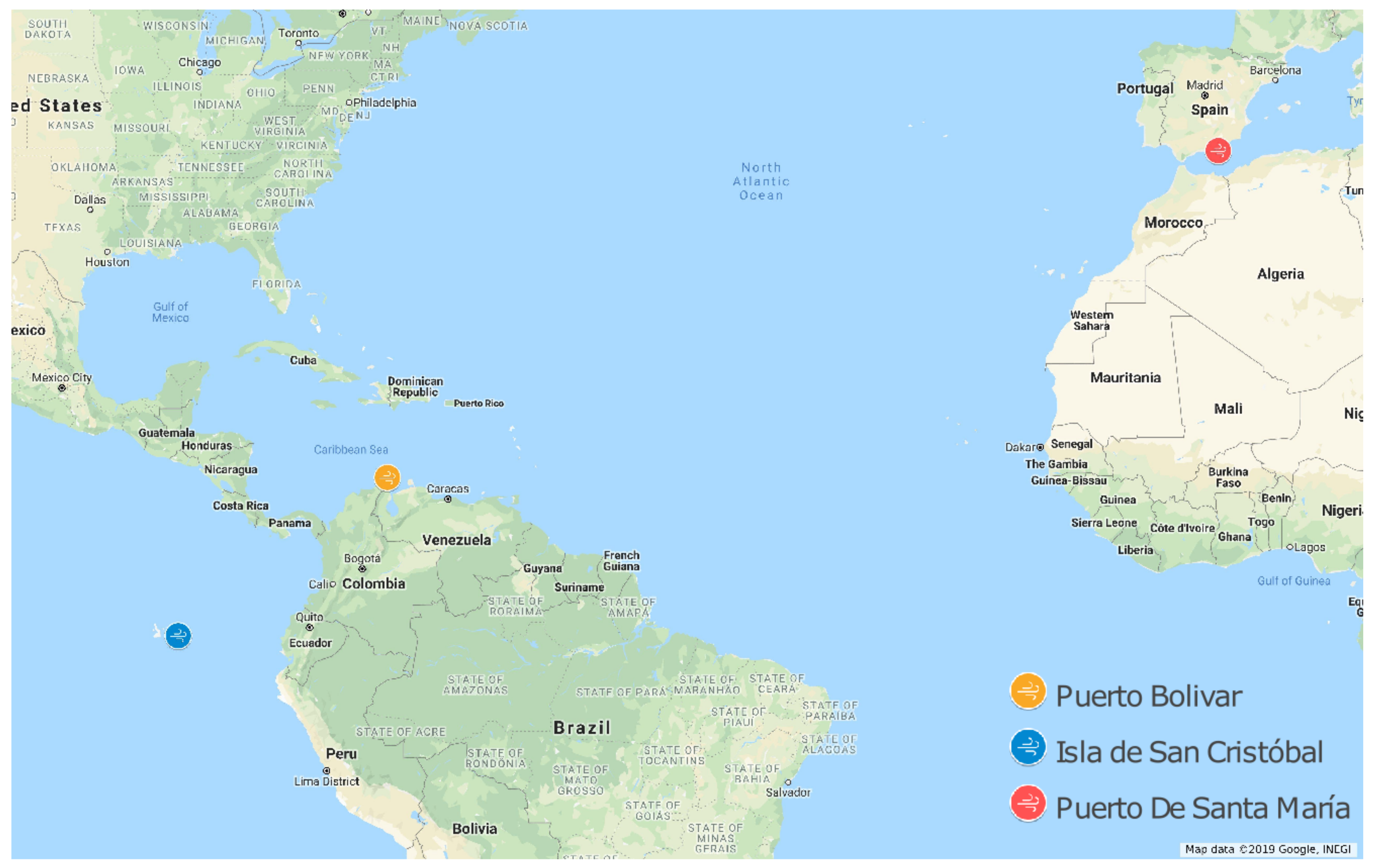
3.1. Test Case
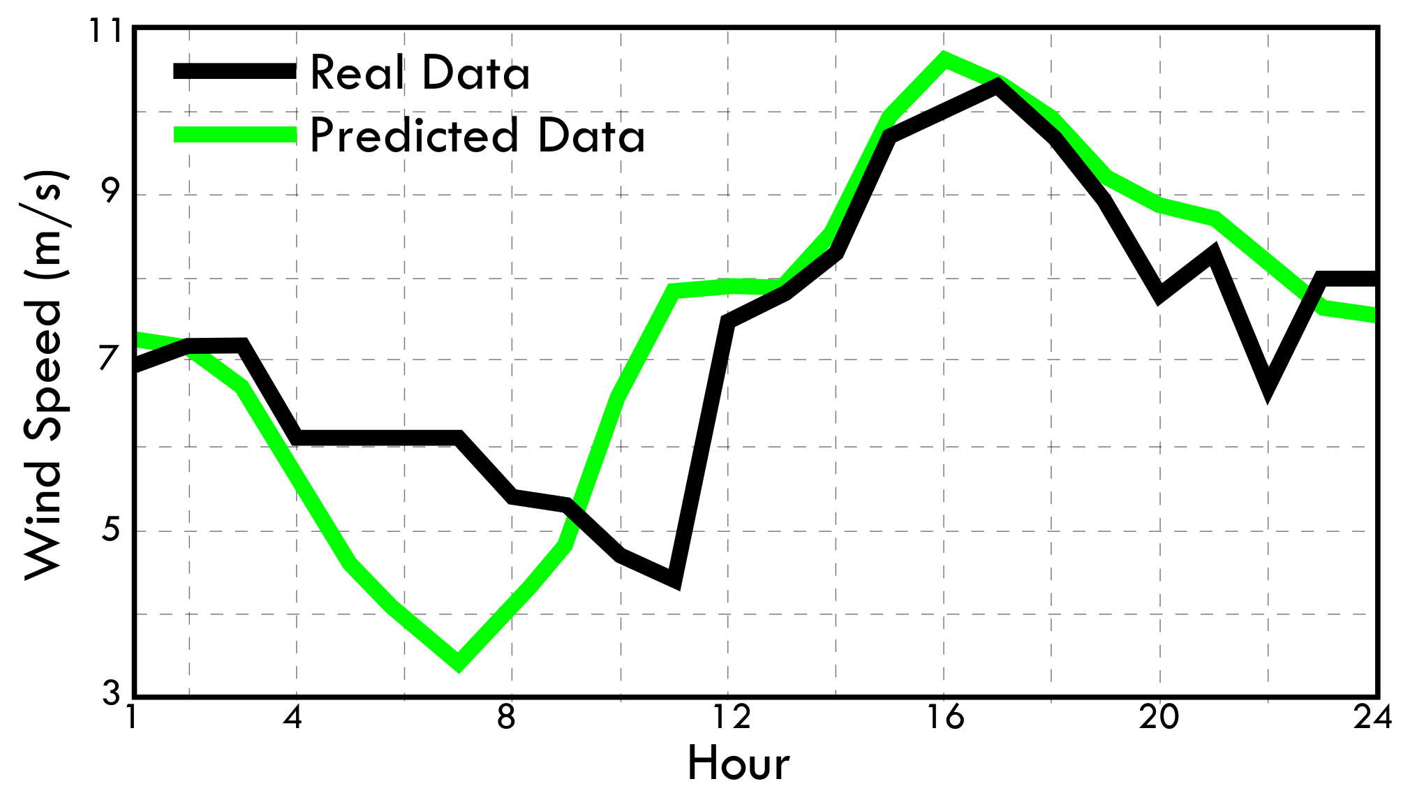
3.2. Results
- Method I: LSSVM
- Method II: WT-LSSVM-REC
- Method VI: Autoregressive simple
- Method VII: LSSVM
- Method VIII: WT-REC-LSSVM
4. Conclusions
Author Contributions
Funding
Acknowledgments
Conflicts of Interest
References
- Perea-Moreno, M.A.; Hernandez-Escobedo, Q.; Perea-Moreno, A.J. Renewable energy in urban areas: Worldwide research trends. Energies 2018, 11, 577. [Google Scholar] [CrossRef]
- Hache, E.; Palle, A. Renewable energy source integration into power networks, research trends and policy implications: A bibliometric and research actors survey analysis. Energy Policy 2019, 124, 23–35. [Google Scholar] [CrossRef]
- Kumar, Y.; Ringenberg, J.; Depuru, S.S.; Devabhaktuni, V.K.; Lee, J.W.; Nikolaidis, E.; Andersen, B.; Afjeh, A. Wind energy: Trends and enabling technologies. Renew. Sustain. Energy Rev. 2016, 53, 209–224. [Google Scholar] [CrossRef]
- Wind, G.; Council, E. Global Wind Report 2019. Available online: https://gwec.net/global-wind-report-2019/ (accessed on 20 November 2020).
- The World Bank. Jepirachi Carbon Off Set Project in Colombia (2002–2024). Available online: https://projects.worldbank.org/en/projects-operations/project-detail/P074426 (accessed on 13 February 2020).
- Ochoa Suárez, M. Energía EóLica: Un Tema de Alto Voltaje para los Wayú. Press Article. Semana. 14 January 2020. Available online: https://sostenibilidad.semana.com/impacto/articulo/energia-eolica-un-tema-de-alto-voltaje-para-los-wayu/47189 (accessed on 13 February 2020).
- UPME. Unidad de Planeación Minero-Energética—Ministerio de Minas y Energía de Colombia. Available online: https://www1.upme.gov.co (accessed on 13 February 2020).
- UPME. Guía Práctica para la Aplicación de los Incentivos Tributarios de la Ley 1715 de 2014. Available online: https://www1.upme.gov.co/Documents/Cartilla_IGE_Incentivos_Tributarios_Ley1715.pdf (accessed on 20 April 2020).
- Comision de Regulacion de Energia y Gas. Código de Redes; CREG Online. Available online: http://apolo.creg.gov.co/Publicac.nsf/Indice01/Resoluci%C3%B3n-1995-CRG95025 (accessed on 20 November 2020).
- Perera, A.T.; Wickramasinghe, P.U.; Scartezzini, J.L.; Nik, V.M. Integrating renewable energy technologies into distributed energy systems maintaining system flexibility. In Proceedings of the 5th International Symposium on Environment-Friendly Energies and Applications, EFEA, Rome, Italy, 24–26 September 2018; IEEE: Piscataway, NJ, USA, 2019; pp. 1–5. [Google Scholar] [CrossRef]
- Huang, C.J.; Kuo, P.H. A short-term wind speed forecasting model by using artificial neural networks with stochastic optimization for renewable energy systems. Energies 2018, 11, 2777. [Google Scholar] [CrossRef]
- Dolatabadi, A.; Jadidbonab, M.; Mohammadi-Ivatloo, B. Short-Term Scheduling Strategy for Wind-Based Energy Hub: A Hybrid Stochastic/IGDT Approach. IEEE Trans. Sustain. Energy 2019, 10, 438–448. [Google Scholar] [CrossRef]
- Ackermann, T. Wind Power in Power Systems; Wiley Online Library: Hoboken, NJ, USA, 2005; Volume 140. [Google Scholar]
- Fallis, A. Developing wind power projects: Theory and Practice. J. Chem. Inf. Model. 2013, 53, 1689–1699. [Google Scholar]
- Famoso, F.; Brusca, S.; D’Urso, D.; Galvagno, A.; Chiacchio, F. A novel hybrid model for the estimation of energy conversion in a wind farm combining wake effects and stochastic dependability. Appl. Energy 2020, 280, 115967. [Google Scholar] [CrossRef]
- Borunda, M.; Rodríguez-Vázquez, K.; Garduno-Ramirez, R.; de la Cruz-Soto, J.; Antunez-Estrada, J.; Jaramillo, O.A. Long-term estimation of wind power by probabilistic forecast using genetic programming. Energies 2020, 13, 1885. [Google Scholar] [CrossRef]
- Hu, H.; Wang, L.; Tao, R. Wind speed forecasting based on variational mode decomposition and improved echo state network. Renew. Energy 2021, 164, 729–751. [Google Scholar] [CrossRef]
- Bai, Y.; Tang, L.; Fan, M.; Ma, X.; Yang, Y. Fuzzy First-Order Transition-Rules-Trained Hybrid Forecasting System for Short-Term Wind Speed Forecasts. Energies 2020, 13, 3332. [Google Scholar] [CrossRef]
- Aly, H.H. An intelligent hybrid model of neuro Wavelet, time series and Recurrent Kalman Filter for wind speed forecasting. Sustain. Energy Technol. Assessments 2020, 41, 100802. [Google Scholar] [CrossRef]
- Chang, W.Y. A Literature Review of Wind Forecasting Methods. J. Power Energy Eng. 2014, 2, 161–168. [Google Scholar] [CrossRef]
- Liu, D.; Niu, D.; Wang, H.; Fan, L. Short-term wind speed forecasting using wavelet transform and support vector machines optimized by genetic algorithm. Renew. Energy 2014, 62, 592–597. [Google Scholar] [CrossRef]
- Catalão, J.P.; Pousinho, H.M.; Mendes, V.M. Short-term wind power forecasting in Portugal by neural networks and wavelet transform. Renew. Energy 2011, 36, 1245–1251. [Google Scholar] [CrossRef]
- Wang, J.; Qin, S.; Zhou, Q.; Jiang, H. Medium-term wind speeds forecasting utilizing hybrid models for three different sites in Xinjiang, China. Renew. Energy 2015, 76, 91–101. [Google Scholar] [CrossRef]
- Liu, H.; wei Mi, X.; fei Li, Y. Wind speed forecasting method based on deep learning strategy using empirical wavelet transform, long short term memory neural network and Elman neural network. Energy Convers. Manag. 2018, 156, 498–514. [Google Scholar] [CrossRef]
- Liu, Y.; Guan, L.; Hou, C.; Han, H.; Liu, Z.; Sun, Y.; Zheng, M. Wind power short-term prediction based on LSTM and discrete wavelet transform. Appl. Sci. 2019, 9, 1108. [Google Scholar] [CrossRef]
- Gomez-Luna, E.; Aponte Mayor, G.; Pleite Guerra, J.; Silva Salcedo, D.F.; Hinestroza Gutierrez, D. Application of wavelet transform to obtain the frequency response of a transformer from transient signals—Part 1: Theoretical analysis. IEEE Trans. Power Deliv. 2013, 28, 1709–1714. [Google Scholar] [CrossRef]
- Bokde, N.; Feijóo, A.; Villanueva, D.; Kulat, K. A review on hybrid empirical mode decomposition models for wind speed and wind power prediction. Energies 2019, 12, 254. [Google Scholar] [CrossRef]
- Huang, N.E.; Shen, Z.; Long, S.R.; Wu, M.C.; Snin, H.H.; Zheng, Q.; Yen, N.C.; Tung, C.C.; Liu, H.H. The empirical mode decomposition and the Hubert spectrum for nonlinear and non-stationary time series analysis. Proc. R. Soc. A Math. Phys. Eng. Sci. 1998, 454, 903–995. [Google Scholar] [CrossRef]
- Cherkassky, V.; Ma, Y. Practical selection of SVM parameters and noise estimation for SVM regression. Neural Netw. 2004, 17, 113–126. [Google Scholar] [CrossRef]
- Kuh, A.; Manloloyo, C.; Corpuz, R.; Kowahl, N. Wind prediction using complex augmented adaptive filters. In Proceedings of the 1st International Conference on Green Circuits and Systems, ICGCS, Shanghai, China, 21–23 June 2010; pp. 46–50. [Google Scholar] [CrossRef]
- Wang, X.; LI, H. Multiscale prediction of wind speed and output power for the wind farm. J. Control Theory Appl. 2012, 10, 251–258. [Google Scholar] [CrossRef]


Publisher’s Note: MDPI stays neutral with regard to jurisdictional claims in published maps and institutional affiliations. |
© 2020 by the authors. Licensee MDPI, Basel, Switzerland. This article is an open access article distributed under the terms and conditions of the Creative Commons Attribution (CC BY) license (http://creativecommons.org/licenses/by/4.0/).
Share and Cite
Lopez, L.; Oliveros, I.; Torres, L.; Ripoll, L.; Soto, J.; Salazar, G.; Cantillo, S. Prediction of Wind Speed Using Hybrid Techniques. Energies 2020, 13, 6284. https://doi.org/10.3390/en13236284
Lopez L, Oliveros I, Torres L, Ripoll L, Soto J, Salazar G, Cantillo S. Prediction of Wind Speed Using Hybrid Techniques. Energies. 2020; 13(23):6284. https://doi.org/10.3390/en13236284
Chicago/Turabian StyleLopez, Luis, Ingrid Oliveros, Luis Torres, Lacides Ripoll, Jose Soto, Giovanny Salazar, and Santiago Cantillo. 2020. "Prediction of Wind Speed Using Hybrid Techniques" Energies 13, no. 23: 6284. https://doi.org/10.3390/en13236284
APA StyleLopez, L., Oliveros, I., Torres, L., Ripoll, L., Soto, J., Salazar, G., & Cantillo, S. (2020). Prediction of Wind Speed Using Hybrid Techniques. Energies, 13(23), 6284. https://doi.org/10.3390/en13236284