Improving Convergence in Therapy Scheduling Optimization: A Simulation Study


1
Lab. Simulación y Modelado, Centro de Investigación en Computación (CIC) del Instituto Politécnico Nacional, IPN, Av. Miguel Othon de Mendizabal s/n. Col. La Escalera, Ciudad de México CP 07738, Mexico
2
Área de Física de Procesos Irreversibles, Departamento de Ciencias Básicas, Universidad Autónoma Metropolitana, U-Azcapotzalco, Av. San Pablo 180, Col. Reynosa, Ciudad de México CP 02200, Mexico
*
Author to whom correspondence should be addressed.
Mathematics 2020, 8(12), 2114; https://doi.org/10.3390/math8122114
Submission received: 29 September 2020
/
Revised: 10 November 2020
/
Accepted: 12 November 2020
/
Published: 26 November 2020
(This article belongs to the Special Issue Dynamical Systems and Optimal Control)
Abstract
:The infusion times and drug quantities are two primary variables to optimize when designing a therapeutic schedule. In this work, we test and analyze several extensions to the gradient descent equations in an optimal control algorithm conceived for therapy scheduling optimization. The goal is to provide insights into the best strategies to follow in terms of convergence speed when implementing our method in models for dendritic cell immunotherapy. The method gives a pulsed-like control that models a series of bolus injections and aims to minimize a cost a function, which minimizes tumor size and to keep the tumor under a threshold. Additionally, we introduce a stochastic iteration step in the algorithm, which serves to reduce the number of gradient computations, similar to a stochastic gradient descent scheme in machine learning. Finally, we employ the algorithm to two therapy schedule optimization problems in dendritic cell immunotherapy and contrast our method’s stochastic and non-stochastic optimizations.
1. Introduction
Therapy schedules comprise previously planned protocols of injection times with their respective vaccine quantity. Such protocols are proposed usually following therapist traits such as intuition and experience. We aim to provide a rational therapy planning that relies on mathematical modeling, optimal control, and simulations.
Optimal control is a popular tool to improve schedules for tumor treatment, and it is frequently used to rationalize issues like infusion times and drug quantities. For instance, in [1], they address the optimal control for a model with mixed immunotherapy and chemotherapy. Numerical and analytic control techniques for continuous and bang-bang controls can be consulted in [2]. Therapeutic protocol improvement by simulations have been made in [3] for Cytotoxic T Cell (CTL) and in [4] for dendritic cell transfections.
Apart from immunotherapy applications, optimal control is used in a variety of medical applications such as control of Dengue Fever [5] time valuation in chronic myeloid leukemia [6], for finding the best therapy schedule for metastatic castrate-resistant prostate cancer using abiraterone [7]. In [8], an optimal control scheme aids the effector cells and Interleukin-2 (IL-2) intensity while lessening the tumor cells. A mathematical model for Chronic myeloid leukemia and optimal control are used in [9] to obtain optimal piecewise-constant regimens. For a combination of therapies, optimal control can be used to find the optimal treatment between several drug options, in [10] dominant treatment is found for the combination of chemotherapy, IL-2, and tumor-infiltrating lymphocyte, considering the tumor size. Ref. [2] discuss several numerical and analytic control techniques for continuous and bang-bang controls. The works [8,11,12], study models for tumor growth, the immune system, and controlled drug therapies given in a Bang-Bang manner.
Standard procedures for taking anti-tumor medicament is to have an intramuscular shot or an intravenous injection. In both cases, the periods for drug intake is on the order of minutes or hours for intravenous intake. Hence, to implement continuous and bang-bang controls that usually need the treatment to stay continually over days is unrealistic. In this paper, we do not consider a continuous-infusion therapy, but pulse-like doses of short period (bolus injection) that can be considered instantaneous. This resembles more accurately the procedure following real immunotherapy treatments. Periodically pulsed immunotherapy is studied on [13,14] where the bolus injections have very small time-span in comparison with the overall therapy. A therapy-optimizing algorithm for pulsed dendritic immunotherapy is given in [15]; also, they give the foundation for computing the gradient of a cost function that measures tumor outgrowth. Schedule optimization for pulsed dendritic immunotherapy that encounters several impediments in the host environment, such as immunosuppression and poor transference to the lymph nodes is addressed on [16]. Then, deciding when and how much of such doses is a typical question when dealing with immunotherapy.
Gradient descent (GD) optimization algorithm is commonly used for schedule optimization when there are pulsed controls [15,16]. The algorithm has many good qualities, but speed convergence is not one of them. Considering that, we change the GD design in our method and use adaptive optimizations that are well known in the area of deep learning and we show that they can be useful too in the area of therapy scheduling for speeding up convergence. It was possible since such approaches rely on the gradient calculation given in [15]. Moreover, we included a stochastic step for decrease the number of gradient computations.
The road-map for this work is as follows. The explanation of the Gradient descent and its variants are in Section 2. Section 3 contains the optimal control problem and the optimization algorithm, followed by Section 4, that has a comparison between the GD variants for an application to a dendritic vaccine schedule model. Also, Section 4 has a comparison between the deterministic case and stochastic cases of the optimization algorithm. Section 5 applies the algorithm for a model calibrated to match the tumor growth in mice. It shows that the stochastic case can give reasonable results with a less computational cost. Finally, on Section 6 have some conclusions and future work.
2. Gradient Descent Optimization Algorithms
In this section, we describe the background for the gradient descent algorithm and some well know optimization algorithms, each version aims to speed up the convergence.
Gradient descent (GD) is an algorithm to find a minimum of a smooth function J using the iterative process:
that take small steps in the gradient . The updating of vector follows the opposite direction of the gradient, and the parameter h gives the step amount the update. For a sufficiently small h and a convex function J, Equation (1) will converge to a global minimum, and for non-convex function is only guaranteed to converge in a local minimum. Step size h plays a vital role in the optimization process; h must give a balance between speed and convergence in the optimization. The procedure includes to test some value for for a few optimizations steps if the loss function decreases fast enough is elected, if not, h is increased a little. Usually, h is small initially, values such as are common in the literature; nevertheless, the range of h differs between different problems. For example, in Section 4 we found that provides us an acceptable convergence in our problem.
For its versatility and simplicity, GD is the workhorse algorithm for a vast number of applications in areas such as mechanics, economics, physics, and machine learning. Equation (1) sometimes is also called vanilla GD for its simplicity.
2.1. Variants
Next, we summarize some adaptive optimization techniques that aim to improve the speed convergence of the GD algorithm. Most of them are thoroughly used and identified in deep learning to fit the parameters of a neural network. The following GD variants (or usually called optimizers) have helped deep learning to improve the state-of-the-art of computer vision, speech recognition, and drug discovery [17]. All of them tweak the GD algorithm to speed up and smooth convergence in distinct forms. We use ⊙ (Hadamard Product) for element-wise vector multiplication; and, square root and division operation on vectors are element-wise operations for the sake of simplicity.
2.1.1. Momentum
GD has difficulty to reach an optimum because of its inclination to oscillate on steep surface curves [18]. Momentum intends to add inertia and speed while also dampening oscillations; like a snowball that passes through minor bumps but stays on the valley. The method of momentum [19] accelerates iterations in such cases. Now, the gradient affects position indirectly through a so-called velocity vector v,
In practical terms, the updated position now depends on the past iteration of v and on the current gradient . The term has a dampening and speeding up effect on s similar to a snowball down a valley. When the snowball is rolling in a pronounce slope, the velocity increases until it reaches the bottom where the velocity decays.
2.1.2. Nesterov
Similar to momentum, this method not only looks at the past velocity but also into the possible next iteration of the momentum update, this takes the form
The reasoning is, that since momentum is about to push s by , then, it make sense to approximate on the direction .
2.1.3. Adagrad
Adagrad optimizer adapts the step size to use past gradient values. At each step a buffer variable b accumulates the squared sum of past gradients,
Now each element s will experience different step size, elements with high gradients will have their step size reduced, and those with smaller gradients will have increased. It has been observed that using the square in the denominator make the algorithm to perform better [19]. Also, serves as a smoothing term for preventing division by zero. Notice that at each optimization step, b adds a positive term which could make b to grow so big that the current step size becomes too small and prevent further advance.
2.1.4. RMSprop
To cope with diminishing step size of Adagrad optimizer the buffer variable includes a decay rate to smooth the impact from big gradients and the accumulative sum,
popular default values for the decay rate are . Now the active step size does not get monotonically smaller [19].
2.1.5. Adam and Adam-Bias
These optimizers combine a smooth version of momentum with RMSprop to adjust the update step h element-wise. Now we have a decaying mean (first moment) of past gradients,
The RMSprop part is the same,
and relates to the uncentered variance (second moment). The Adam optimizer is usually presented as,
and the one called Adam-bias optimizer as
where the variables are for correcting potential bias toward zero of . The name Adam comes from Adaptive Moment Estimator [20] in which they proposevalues of for and for .
2.1.6. GD-Normalized
In our experiments, the elements of tend to differ several orders of magnitude, so, step size h could be either significant or negligible in the updating. To smooth that effect, we include a version that normalizes the gradient before making the schedule update;
we call this GD-Normalized. For further discussion on the above methods, we refer to [21].
3. The Optimal Control Algorithm for Optimizing Therapy Schedules
In this section, we define the optimal control problem for therapy scheduling and an algorithm for optimizing therapy schedules using GD. This algorithm includes a stochastic step that only updates a random part of the schedule at each iteration. This simple technique gives us similar results on minimizing a cost function J in comparison with updating the entire schedule at each step. The advantage is that it has less computational cost.
3.1. The Optimal Control Problem Definition
The clinical effectiveness of immunotherapy vaccines by simulations of mathematical representations is a theme of open-ended research in mathematical oncology [22]. One of the most used tools for modeling the complex interactions between the immune system, tumor cells, and external therapies is ordinary differential equations (ODEs). With the mathematical model, hypothetical protocols simulation can proceed with several therapy combinations of dose timing and size. Such protocols could lead to new therapy dosing programs [4]. For this section we improve such hypothetical protocols using an optimization algorithm based on optimal control.
The treatment is modeling by a system of ODEs that depends in the control u,
where x is the state variable and u measures the therapy effect. For this work, u will act only in one of the independent variables of (20). Also, let be defined as the coordinate vector with i equal to the index of such independent variable. For example we would have for the system (24)–(28). Now, let us consider a schedule of injections be given as,
such that , with as the therapy fixed starting point and, is the therapy fixed end. It is considered that a therapeutic protocol consists of n doses of size V given by the times on s. Let be the space of schedules, then for a particular schedule the control variable takes the form:
Notice, we are approximating the doses as an impulse given by the Dirac function . For this work, we will focus on a cost function of the form,
where L measures how effective is the running therapy and measure the cost at the end of the therapy. The optimal control problem consists in:
- (P) Determine the schedule of n injectionsthat solves;
3.2. Optimization Algorithm
The Algorithm 1 uses the same method reported in [15] to compute the gradients of J. Since the methods in Section 2 are guaranteed to converge for convex problems and the applications in this work are for nonlinear dynamics (non-convex) the Algorithm 1 acts as a heuristic. Additionally, we also study the case when a schedule is randomly chosen from s.
| Algorithm 1: Schedule Optimization with stochastic step |
|
In step S3 of Algorithm 1, the correct decision of h is essential. If h is very big, we could not see progress, if h is too insignificant, the optimization could develop slowly. The S3 step is the vanilla GD indicated by (1). Step S3 can be interchanged for any optimization algorithm of Section 2 The choice of those optimization algorithms has a significant impact on the number of optimization steps needed to reach the minimum, as we will observe in the next section. Vanilla GD is the optimization algorithm found in the literature for schedule optimization using optimal pulsed control [15,23].
Notice that for each optimization step (S1–S3) we are letting time injection values with no updating. That lightens the number of gradient computations on each step. From our simulations, whenever Algorithm 1 converges to a minimum using it will also converge with , but further exploration is needed to define the lower bound for p to make certain minimum reaching. Using and vanilla GD equation, we restore the algorithm used in [15,16]. Also, Algorithm 1 resembles the Stochastic Gradient Descent (SGD) algorithms adopted in deep learning applications. SGD involves updating a parameter vector from a subset of training samples randomly chosen (mini-batch) instead of the whole training set. A drawback of SGD is that the cost function shows high fluctuations while is updating; the smallest the mini-batch, the higher the fluctuations. We discover analogous behavior in our schedule evolution.
4. Application to a Dendritic Vaccine Schedule for Tumor Cells Model
This section has the optimization of two initial therapy schedules, one with a few injections times and another with daily doses over six months. We compare the gradient descent variants presented in Section 2 with attention on convergence speed-up. Algorithm 1 use the next mathematical model which accounts for tumor-immune and dendritic vaccine interactions, further details and parameters can be found in [23],
which has 5 state variables:
- T, the tumor cells.
- H, the T helper cells.
- C, the T or cytotoxic cells.
- D, the antigen loaded dendritic cells.
- I, the Interleukin-2 cytokine.
In this section, Algorithm 1 aims to minimize the cost function,
where is the solution of (24)–(28). Notice that the running cost,
measure how much cancer cells T goes beyond the threshold , and the final cost measures the number of cancer cells at the end. Then, the optimizer penalizes schedules that let go above while making as small as possible.
4.1. Optimization and Comparison of GD Variants
In this subsection, we compare the GD extensions from Section 2 on Algorithm 1 to minimize the cost function in Equation (29).
We do two optimization runs, one for (Figure 1) and other for (Figure 2) with the initial schedule;
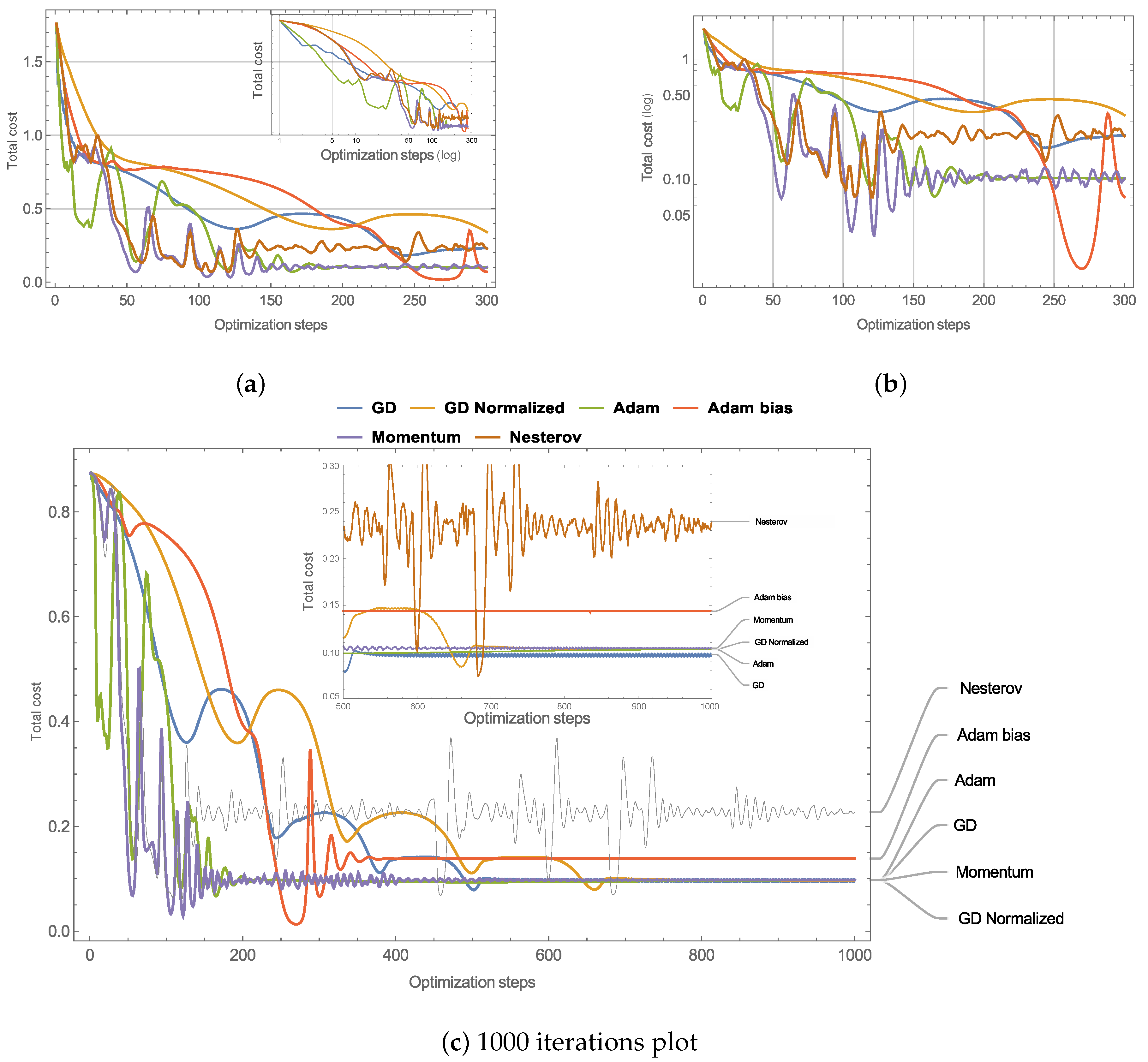
with doses of . From Figure 1a miniature GD has faster first decay but Adam variant quickly outperforms it. Most of the optimizers oscillate after step 50 except for GD and GD-Normalized which has a slower convergence. The first to converge is Adam to the minimum , and momentum to converge to too but stays in a decreasing oscillatory behavior. Adam-bias has a moderate initial convergence, but after step 225 it decreases fast going below , although it converges to approximately until step 400 (Figure 1c). From Figure 1b, we can appreciate that Adam and Momentum converge to a local minimum of roughly .
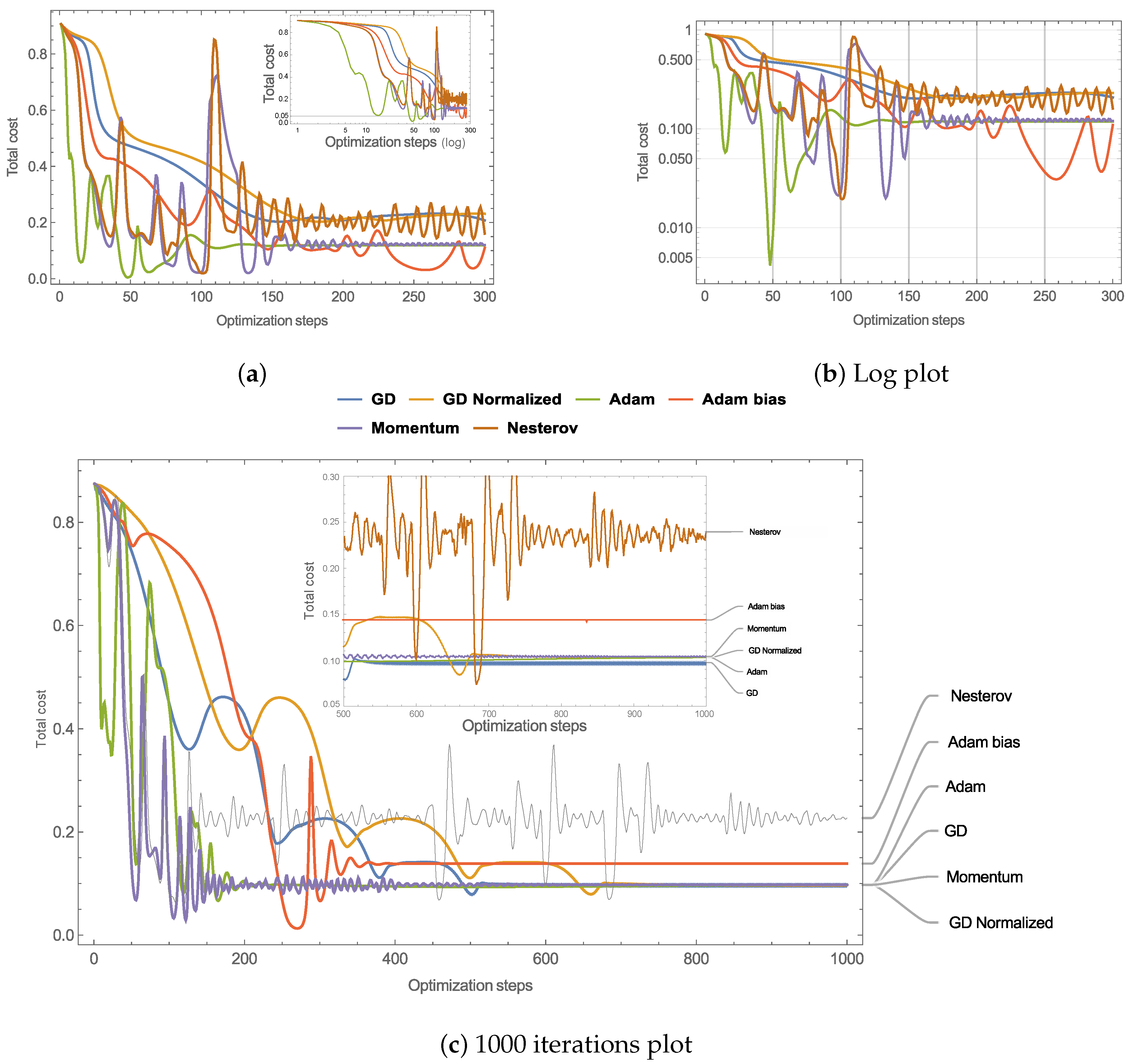
For the case Figure 2 shows similar results than the case . Adam has the faster initial decay, goes below on about 15 optimization steps but oscillates back and forth several times, then goes below on about 50 optimization steps (Figure 2b). The miniature of (Figure 2c) shows Momentum and Adam variants converging to the same value . Nesterov variant oscillates around and never settles down. The variant GD-Normalized converges to until 650 optimizations steps where it shows small fluctuations. On the other hand, GD converges to until 800 optimization steps.
Cases and presents many oscillations which are very common in algorithms using momentum-like optimization [18], and this probably can be adjusted with a different parameter choice for Adam, Momentum, and Nesterov. Vanilla GD and GD-Normalized do not present prominent oscillations but present a slower convergence. Table 1 shows the parameter election for each optimization variant.
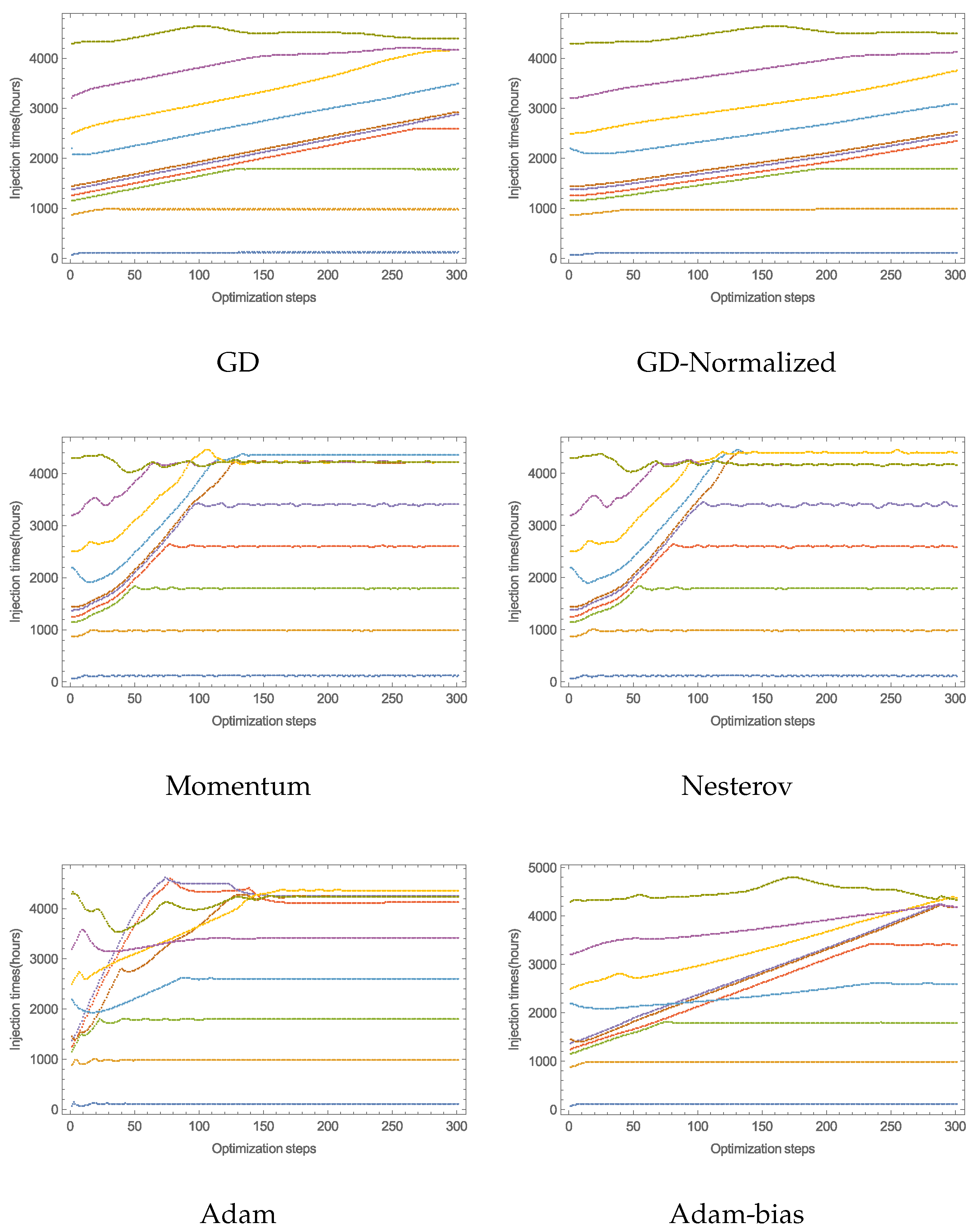
Figure 3 shows the schedule evolution for each GD variant. At each iteration, each optimizer moves to try to minimize the cost function J. The abscissa shows the number of optimization steps, and the ordinate shows the administration times in hours. On the whole, each GD variant favors an accumulation at the end of the therapy for minimization; also, there are equally spaced injections that contribute to decreasing the running cost. When two or more injection times collapse at roughly the same value, can be interpreted as a single injection with dose size as the sum of every collapsing dose. Figure 3 also reveals the difference between the convergence of the GD variants, Adam variant moves a lot faster the injection times to the end of the therapy. Conversely GD and GD-Normalized have little effect on the initial schedule; nonetheless, they also show a tendency to move injection times to the end. Nesterov and Momentum have a similar evolution, expected as they are very similar. Unexpectedly, Adam-bias evolve a lot slower than Adam, probably Equations (12) and (13) do not start biased towards zero, and the adaptive step size coming from dividing by hinders the convergence. Next, it is explored the case for daily doses for six months.
Daily Doses over Six Months
Now, we optimize a more extensive first schedule over six months (4320 h). It comprises daily injections of dose size , with a total dose of 3 roughly. Here we use the same cost function of Equation (29). We use Algorithm 1 deterministically with and stochastically with . Also, it is run for 300 optimizations steps using Adam variant with , , .
Notice that smaller values for p mean less computational cost. Let N be the fixed number of optimizations steps and . Then the total number of gradient calculations are given by;
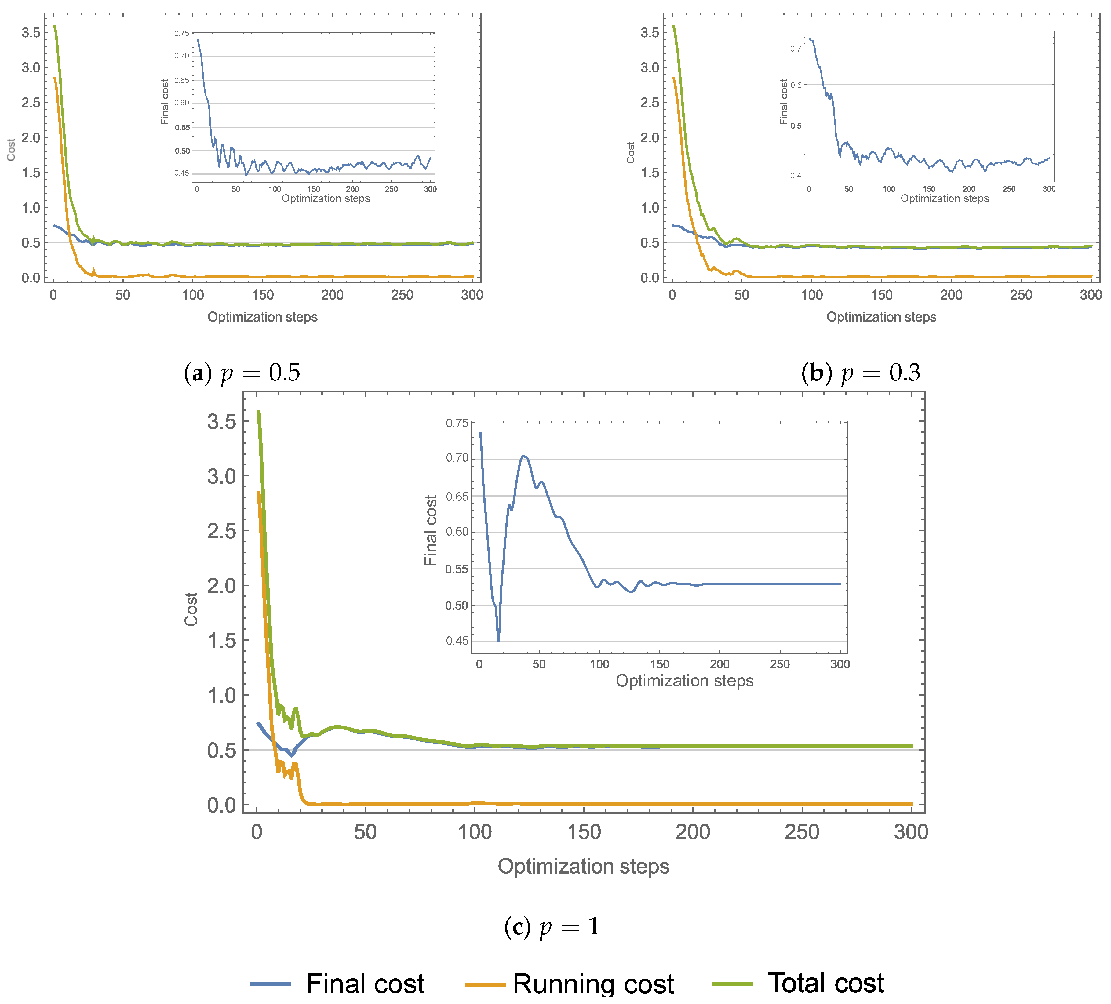
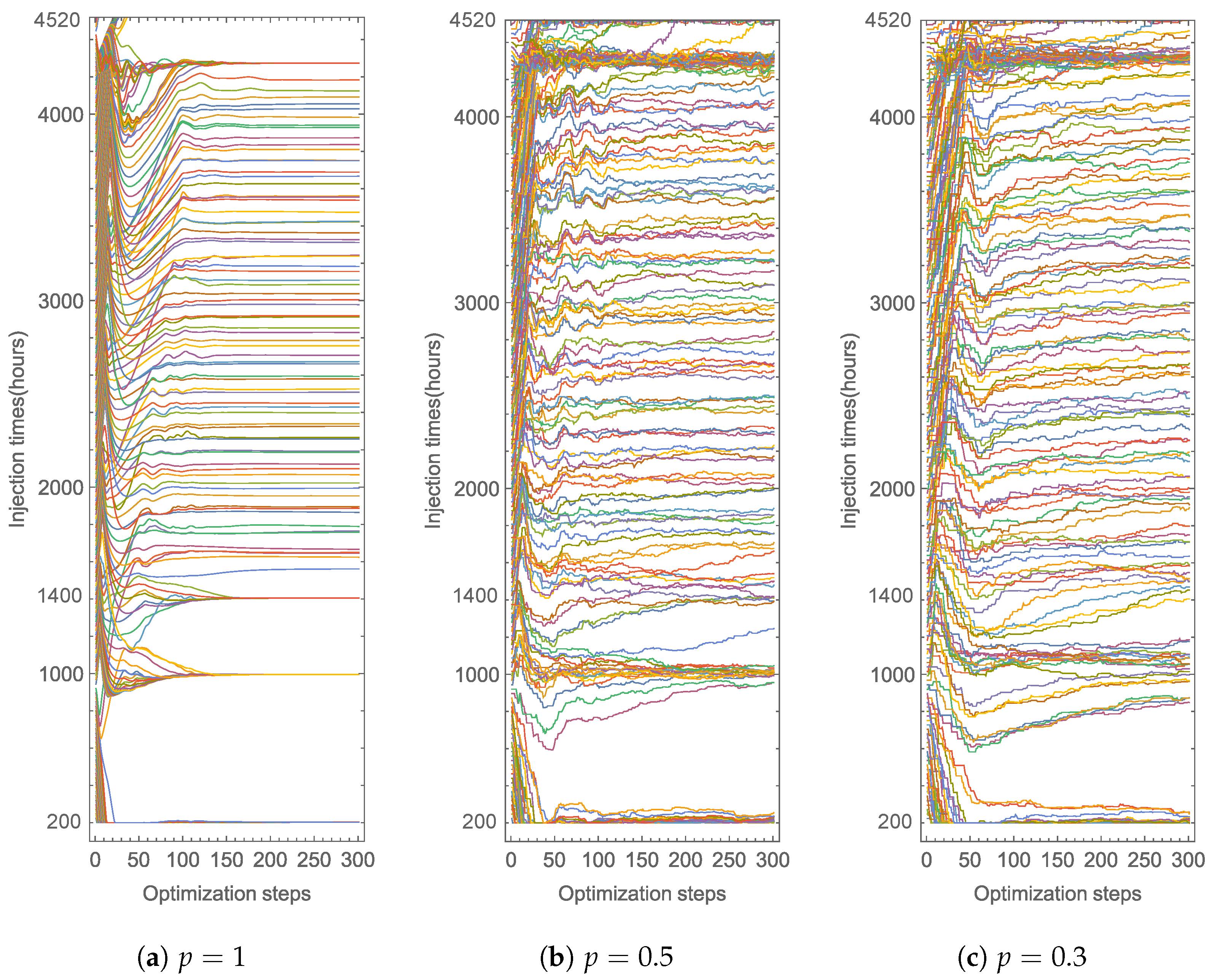
For this example, using make cost function to converge to the same minima. Figure 4 displays the plots of minimization for cost functions J using . For the three cases the running cost and the total cost looks very similar, on the other hand, the final cost (the miniatures) does not. The running cost for each instance decays quickly to . But, for case running cost fluctuate at the 10–20 optimization steps, then converges near to until step 100. The final cost causes these fluctuations (better shown in the miniatures), jumping up when it reaches and stabilizing until step 150 onto . Random cases in contrast, final cost for decays and fluctuates inside the interval and for inside interval . Consequently, stochastic instances display slightly better total cost, because their final cost is below deterministic case final cost. Furthermore, random instances have fewer gradient computations. For instance, since gives = 54,000, gives = 27,000, and for we have = 16,200. Hence, the stochastic versions only compute the and of the gradients when .
Figure 5 displays the corresponding schedule dynamics for the three cases. Therapy starts at t = 200 h and ends after six months at t = 4520 h. For the deterministic case () displays a well defined initial movement towards t = 200 h, 1000 h, 1400 h, 4300 h, 4520 h which continues to accumulate until collapsing into a single time point. Not all injection times combine; between [1400 h, 4300 h] some injection times stay uncombined until the optimization ends. Although Interval [1400 h, 4300 h] presents an accumulation of injections in fewer quantities, in general shows low and frequent doses similar to what is called a metronomic therapy [24]. The accumulation at the start (t = 200 h) and end (t = 4320 h) is because Algorithm 1 let injections to go neither above the fixed end nor below the start. Such restriction was required to obtain successful optimization; Algorithm 1 failed to converge to a minimum when the therapy start and end were variable. So, to optimize a schedule with variable period requires further analysis.
For the stochastic cases in Figure 5a,b, the schedule evolution is less smooth, and in comparison, looks like a perturbed version of the deterministic one. At injection times t = 200 h, 1000 h, 1400 h, 4300 h, 4520 h, there is a tendency to accumulate; and further steps could show a single injection. Notice that inside [1400 h, 4300 h] stochastic and deterministic optimizations have sparse injection times of frequent and low dose. Also, both cases accumulate injections but the deterministic case appears very plain. Notice that both optimization cases present injection times that move in the same direction forming groups, for stochastic versions, that movement looks messy and delayed. That can be explained, considering that some injection times have a deferred update; at each optimization step Algorithm 1 only picks to update % of the injection times from the schedule, for the not chosen, the system is in a different state that if they were updated at once.
Since the deterministic and stochastic variant yields similar schedules, then perhaps the schedule from the deterministic variant is stable to small perturbations.
5. Application for Therapy Schedule Improvement in Murine Model
In this section, we examine a murine mathematical model that deals with the effects of dendritic cell bolus doses, and obstacles in the host environment; such as immunosuppression, and vaccine effect reduction generated by insufficient transference to the lymph nodes. The analyzed model is;
which has 8 state variables:
- T, the tumor cells.
- H, the T helper cells.
- C, the T or cytotoxic cells.
- D, the antigen loaded dendritic cells.
- I, the Interleukin-2 cytokine.
- , the T cell inhibitor.
- , the which up-regulates class 1.
- , is the number class 1 receptors per melanoma cell.
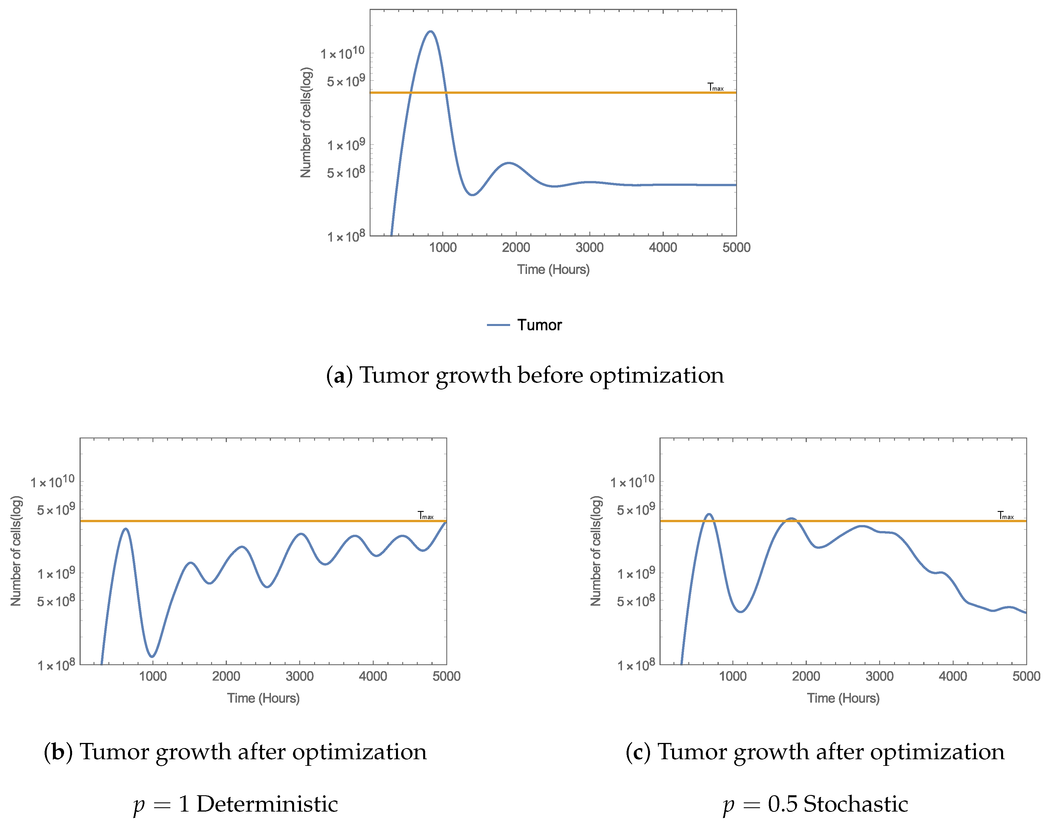
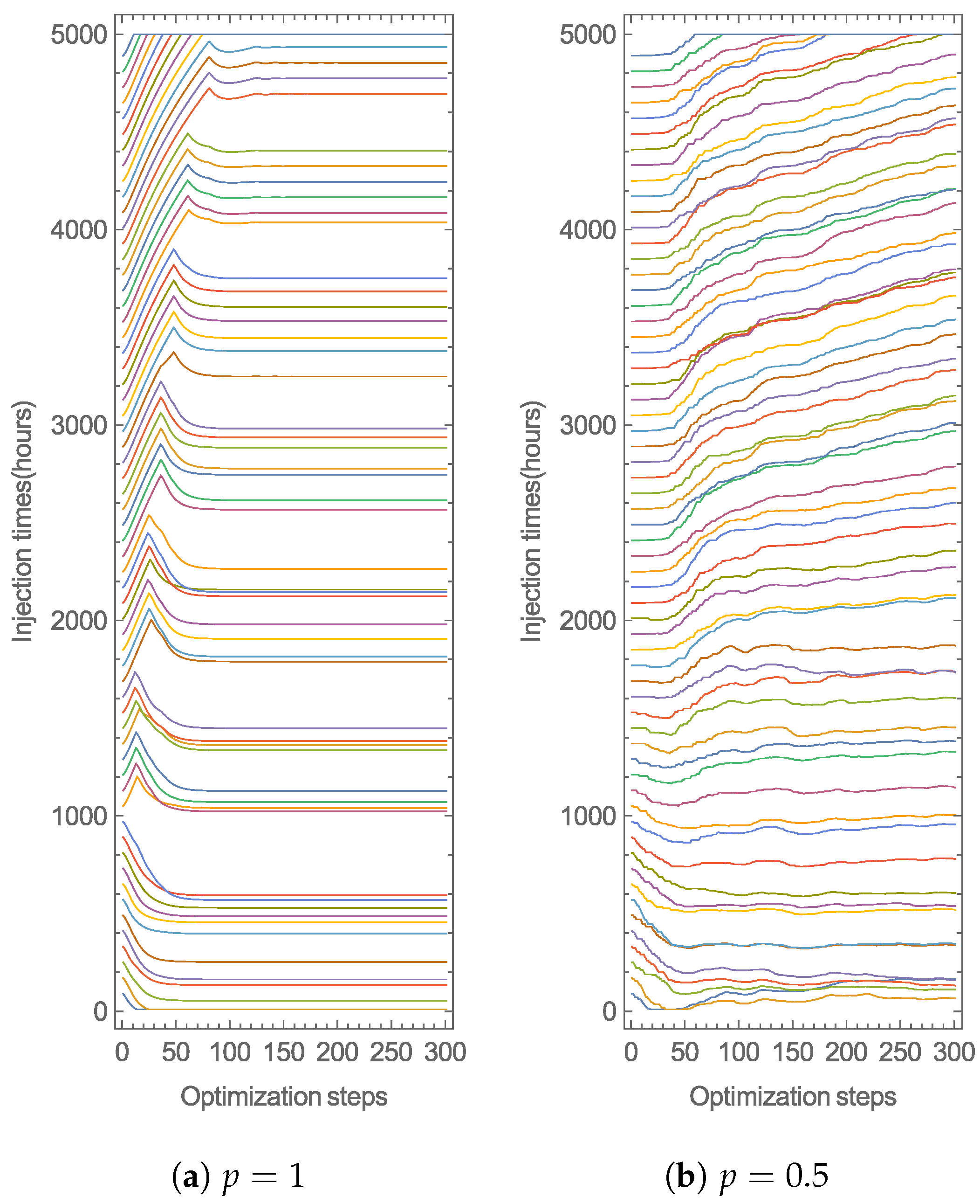
We have calibrated the parameters of this model to the tumor growth data of mice imbued with melanoma cells [25], such parameters and deeper discussion are on [16]. We apply Algorithm 1 to improve a starting schedule , so that the eventual schedule drives the tumor mass to stay under threshold . Figure 6c have 300 optimizations steps using Adam variant with , , and a fixed horizon h. We start with the schedule with injection times every 80 days of amount and overall dosage , where is the portion of dendritic cells that reach to the lymph nodes. Figure 7 indicates the deterministic and stochastic schedule evolution. Deterministic case renews the full schedule in every optimization step, and the stochastic form percent of the time points (). Both optimizations distribute the injections times, so the therapy keeps the number of tumor cells below (Figure 6).
For the deterministic case, the first optimization steps in Figure 7a illustrates a trend for point times to advance to late times, and for move to a early times. This tendency remains until injection times stop evolving, and the following schedule has cycles of frequent doses and periods without doses. For stochastic optimization (Figure 7b), the initial evolution is like the deterministic one, but with tinier updates. After 300 optimization steps, the doses do not stay fix, the injection times can further evolve. The resulting schedule comprises scattered doses over the treatment duration and a few doses of fusions.
Figure 6a displays the tumor expansion for the first dose protocol. There is a considerable tumor growth that surpasses in the period [0 h, 1000 h], later when therapy influence; the tumor decreases and stays about . Figure 6b illustrates tumor growth, reacting to the therapy after schedule optimization with . The optimized schedule drives T to stay below ; however, T stay rising and fluctuating towards the therapy end. Figure 6c (the stochastic optimization) shows that T resides mostly below , except for two instances about t = 600 h, 1800 h. Nonetheless, tumor growth progresses decreasing towards the end. In contrast, the stochastic optimization computed half the gradients computed by the deterministic optimization.
6. Concluding Remarks
In this study, we introduce a stochastic gradient descent technique for optimization problems with pulsed controls and a comparison between several gradient descent extensions. The comparison shows different convergence speeds between optimizers. These methods are well known but have convergence guarantees only for convex problems. However, the problems in Section 4 and Section 5 involve nonlinear dynamics, thus they are non-convex, which makes it difficult to make a rigorous convergence study. We aim to highlight the importance of using adaptive optimization algorithms in these kinds of applications empirically. In Section 4 and Section 5 we show that not every optimization approach will perform as expected, for example, Adam-bias has slower convergence than Adam, when regularly, Adam-bias converges faster on machine learning applications.
In the applications, we employed the method to identify therapy schedules that control tumor volume to stay under a threshold while minimizing tumor volume towards the therapy end. For both applications, the stochastic variant uses fewer gradient computations than the deterministic variation, with comparable results. We apply this method in the cancer treatment scope, but it can be transferred to ODE models with pulsed control that intends to minimize a cost function in the form of Equation (23).
The method presented in this manuscript rationalize the construction of immunotherapy schedules, which could complement therapist intuition and experience in therapy planning. Future work continues the technique for real clinical practice. We aim to optimize dosage and to introduce a penalty term that accounts for timing restrictions, such as weekends and holidays. Experiments on non-fixed time boundaries fail to converge, which calls for further research.
Author Contributions
Conceptualization, J.C.C.-E. and J.C.R.-R.; Formal analysis, J.C.C.-E. and J.C.R.-R.; Investigation, J.C.C.-E.; Methodology, J.C.R.-R.; Software, J.C.R.-R. and R.T.P.-H.; Validation, J.C.C.-E. and J.C.R.-R.; Visualization, J.C.R.-R.; Writing—original draft, J.C.R.-R.; Writing—review and editing, J.C.C.-E. and R.T.P.-H. All authors have read and agreed to the published version of the manuscript.
Funding
Comisión de Operación y Fomento de Actividades Académicas del Instituto Politécnico Nacional (COFAA-IPN, project number 20200606).
Acknowledgments
The authors wish to thank “Consejo Nacional de Ciencia y Tecnología” (CONACyT), “Comisión de Operación y Fomento de Actividades Académicas del Instituto Politécnico Nacional” (COFAA-IPN, project number 20200606) and “Estímulos al Desempeño de los Investigadores del Instituto Politécnico Nacional” (EDI-IPN) for the support given for this work.
Conflicts of Interest
The authors declare no conflict of interest.
References
- De Pillis, L.G.; Fister, K.R.; Gu, W.; Head, T.; Maples, K.; Neal, T.; Murugan, A.; Kozai, K. Optimal control of mixed immunotherapy and chemotherapy of tumors. J. Biol. Syst. 2008, 16, 51–80. [Google Scholar] [CrossRef]
- Schättler, H.; Ledzewicz, U. Optimal control of cancer treatments: Mathematical models for the tumor microenvironment. In Analysis and Geometry in Control Theory and Its Applications; Springer: Cham, Switzerland, 2015; pp. 209–235. [Google Scholar] [CrossRef]
- Kronik, N.; Kogan, Y.; Schlegel, P.G.; Wölfl, M. Improving T-cell immunotherapy for melanoma through a mathematically motivated strategy: Efficacy in numbers? J. Immunother. 2012, 35, 116–124. [Google Scholar] [CrossRef] [Green Version]
- Castillo-Montiel, E.; Chimal-Eguía, J.C.; Tello, J.I.; Piñon-Zaráte, G.; Herrera-Enríquez, M.; Castell-Rodríguez, A.E. Enhancing dendritic cell immunotherapy for melanoma using a simple mathematical model. Theor. Biol. Med. Model. 2015, 12, 1–14. [Google Scholar] [CrossRef] [PubMed] [Green Version]
- Onyejekwe, O.O.; Tigabie, A.; Ambachew, B.; Alemu, A. Application of Optimal Control to the Epidemiology of Dengue Fever Transmission. J. Appl. Math. Phys. 2019, 7, 148–165. [Google Scholar] [CrossRef] [Green Version]
- Gutiérrez-diez, P.J. The effects of time valuation in cancer optimal therapies: A study of chronic myeloid leukemia. Theor. Biol. Med. Model. 2019, 16, 10. [Google Scholar] [CrossRef] [PubMed] [Green Version]
- Cunningham, J.J.; Brown, J.S.; Gatenby, R.A.; Stankova, K. Optimal control to develop therapeutic strategies for metastatic castrate resistant prostate cancer. J. Theor. Biol. 2018, 459, 67–78. [Google Scholar] [CrossRef] [PubMed] [Green Version]
- Ghaffari, A.; Naserifar, N. Optimal therapeutic protocols in cancer immunotherapy. Comput. Biol. Med. 2010, 40, 261–270. [Google Scholar] [CrossRef] [PubMed]
- Moore, H. How to mathematically optimize drug regimens using optimal control. J. Pharmacokinet. Pharmacodyn. 2018, 45, 127–137. [Google Scholar] [CrossRef] [Green Version]
- Head, T.; Maples, K.; Neal, T.; Murugan, A.; Kozai, K. Optimal Control of Mixed Immunotherapy. Optim. Control. Mix. Immunother. 2008, 16, 51–80. [Google Scholar]
- de Pillis, L.G.; Radunskaya, A. A Mathematical Tumor Model with Immune Resistance and Drug Therapy: An Optimal Control Approach. J. Theor. Med. 2001, 3, 79–100. [Google Scholar] [CrossRef] [Green Version]
- De Pillis, L.G.; Radunskaya, A. The dynamics of an optimally controlled tumor model: A case study. Math. Comput. Model. 2003, 37, 1221–1244. [Google Scholar] [CrossRef]
- Wei, H.C. A modified numerical method for bifurcations of fixed points of ODE systems with periodically pulsed inputs. Appl. Math. Comput. 2014, 236, 373–383. [Google Scholar] [CrossRef]
- Wei, H.C.; Yu, J.L.; Hsu, C.Y. Periodically Pulsed Immunotherapy in a Mathematical Model of Tumor, CD4 T Cells, and Antitumor Cytokine Interactions. Comput. Math. Methods Med. 2017, 2017, 2906282. [Google Scholar] [CrossRef] [PubMed] [Green Version]
- Castiglione, F.; Piccoli, B. Optimal control in a model of dendritic cell transfection cancer immunotherapy. Bull. Math. Biol. 2006, 68, 255–274. [Google Scholar] [CrossRef] [PubMed]
- Rangel-Reyes, J.C.; Chimal-Eguía, J.C.; Castillo-Montiel, E. Dendritic Immunotherapy Improvement for an Optimal Control Murine Model. Comput. Math. Methods Med. 2017, 2017. [Google Scholar] [CrossRef] [PubMed] [Green Version]
- LeCun, Y.; Bengio, Y.; Hinton, G. Deep learning. Nat. Methods 2015, 13, 35. [Google Scholar] [CrossRef] [PubMed]
- Goh, G. Why Momentum Really Works. Distill 2017. [Google Scholar] [CrossRef]
- Hinton, G.E. Optimization: How to make the learning go faster. Coursera 2012, 4, 26–31. Available online: https://www.coursera.org/learn/neural-networks/lecture/YQHki/rmsprop-divide-the-gradient-by-a-running-average-of-its-recent-magnitude (accessed on 1 September 2018).
- Kingma, D.P.; Ba, J. Adam: A Method for Stochastic Optimization. arXiv 2014, arXiv:1412.6980. [Google Scholar]
- Goodfellow, I.; Bengio, Y.; Courville, A.; Bengio, Y. Deep Learning; MIT Press: Cambridge, MA, USA, 2016; Volume 1. [Google Scholar]
- Eftimie, R.; Gillard, J.J.; Cantrell, D.A. Mathematical Models for Immunology: Current State of the Art and Future Research Directions. Bull. Math. Biol. 2016, 78, 2091–2134. [Google Scholar] [CrossRef] [Green Version]
- Piccoli, B.; Castiglione, F. Optimal vaccine scheduling in cancer immunotherapy. Phys. A Stat. Mech. Its Appl. 2006, 370, 672–680. [Google Scholar] [CrossRef]
- Scharovsky, O.G.; Mainetti, L.E.; Rozados, V.R. Metronomic chemotherapy: Changing the paradigm that more is better. Curr. Oncol. 2009, 16, 7–15. [Google Scholar] [CrossRef] [PubMed] [Green Version]
- Piñón-Zárate, G.; Herrera-Enríquez, M.Á.; Hernández-Téllez, B.; Jarquín-Yáñez, K.; Castell-Rodríguez, A.E. GK-1 improves the immune response induced by bone marrow dendritic Cells Loaded with MAGE-AX in Mice with Melanoma. J. Immunol. Res. 2015, 2015, 176840. [Google Scholar] [CrossRef] [PubMed]
Figure 1.
Panel (a) The linear plots of the total cost (running cost + final cost) vs optimization steps, using different GD variants and . The miniature is the log plot in the x-axis and shows a detailed view of the first steps. Panel (b) is the logarithmic plot on the y-axis. Panel (c) shows the optimization for 1000 steps. The miniature shows a detailed view of the last 500 steps.

Figure 2.
Panel (a) The linear plots of the total cost (running cost + final cost) for each optimization using several GD variants when . Panel (b) the logarithmic plot. Adam variant shows the faster initial decay and also reaches the smaller minimum at roughly 50 steps. Panel (c) iterations up to 1000 steps.

Figure 3.
Comparison between the distinct schedule evolution of each GD variant ().

Figure 4.
(a) The minimization of the cost function computing of the gradients () at each optimization step. (b) Using () of gradients. (c) Using 30% () of gradients. The smaller figures show the final cost.
Figure 4.
(a) The minimization of the cost function computing of the gradients () at each optimization step. (b) Using () of gradients. (c) Using 30% () of gradients. The smaller figures show the final cost.

Figure 5.
Schedule evolution for . Panel (a), the deterministic case, have Algorithm 1 using . Panel (b) stochastic case is done with Algorithm 1 using , so at each optimization step, the algorithm draws of the doses from the schedule to update. Panel (c) stochastic case made with Algorithm 1 using . The schedule shows fluctuations for the stochastic cases.

Figure 6.
Panel (a) shows the tumor growth using a initial 80-day periodic schedule with dose size over 5000 h using a total dose of . Panel (b) the tumor growth after the optimization of the cost function using , the optimized schedule makes the tumor cells count to stay below . Panel (c) the tumor growth after the optimization of the cost function using the optimized schedule makes the tumor cells count go below for most of the 5000 h. The stochastic case has less final tumor cell count.

Figure 7.
Panel (a), the deterministic case, considers Algorithm 1 using . Panel (b) shows the stochastic case using , so, at each optimization step, the algorithm picks of the injection times from the schedule to update. The deterministic case progresses to well-marked schedules. The stochastic version produces a more scattered schedule than the deterministic.


Table 1.
Parameter selection for each optimization variant.
| Method | Parameters |
|---|---|
| GD | |
| GD Normalized | |
| Adam | , , |
| Adam bias | , , |
| Momentum | , |
| Nesterov Normalized | , |
Publisher’s Note: MDPI stays neutral with regard to jurisdictional claims in published maps and institutional affiliations. |
© 2020 by the authors. Licensee MDPI, Basel, Switzerland. This article is an open access article distributed under the terms and conditions of the Creative Commons Attribution (CC BY) license (http://creativecommons.org/licenses/by/4.0/).
Share and Cite
MDPI and ACS Style
Chimal-Eguia, J.C.; Rangel-Reyes, J.C.; Paez-Hernandez, R.T. Improving Convergence in Therapy Scheduling Optimization: A Simulation Study. Mathematics 2020, 8, 2114. https://doi.org/10.3390/math8122114
AMA Style
Chimal-Eguia JC, Rangel-Reyes JC, Paez-Hernandez RT. Improving Convergence in Therapy Scheduling Optimization: A Simulation Study. Mathematics. 2020; 8(12):2114. https://doi.org/10.3390/math8122114
Chicago/Turabian StyleChimal-Eguia, Juan C., Julio C. Rangel-Reyes, and Ricardo T. Paez-Hernandez. 2020. "Improving Convergence in Therapy Scheduling Optimization: A Simulation Study" Mathematics 8, no. 12: 2114. https://doi.org/10.3390/math8122114
Note that from the first issue of 2016, this journal uses article numbers instead of page numbers. See further details here.