Multi-Year Index-Based Insurance for Adapting Water Utility Companies to Hydrological Drought: Case Study of a Water Supply System of the Sao Paulo Metropolitan Region, Brazil

Abstract

The sustainability of water utility companies is threatened by non-stationary drivers, such as climate and anthropogenic changes. To cope with potential economic losses, instruments such as insurance are useful for planning scenarios and mitigating impacts, but data limitations and risk uncertainties affect premium estimation and, consequently, business sustainability. This research estimated the possible economic impacts of business interruption to the Sao Paulo Water Utility Company derived from hydrological drought and how this could be mitigated with an insurance scheme. Multi-year insurance (MYI) was proposed through a set of “change” drivers: the climate driver, through forcing the water evaluation and planning system (WEAP) hydrological tool; the anthropogenic driver, through water demand projections; and the economic driver, associated with recent water price policies adopted by the utility company during water scarcity periods. In our study case, the evaluated indices showed that MYI contracts that cover only longer droughts, regardless of the magnitude, offer better financial performance than contracts that cover all events (in terms of drought duration). Moreover, through MYI contracts, we demonstrate solvency for the insurance fund in the long term and an annual average actuarially fair premium close to the total expected revenue reduction.

1. Introduction

The link between climate change and the economic impact of natural disasters is a fact that can hardly be contradicted [1]. According to a report published by the World Meteorological Organization [2], from 1971 to 1980 and 2001 to 2010, the number of reported disasters and amount of economic losses by decade increased by factors of 4.7 and 5.5, respectively, despite policy and adaptation actions against climate change that were adopted [3]. The report specified that approximately 11% of natural disasters reported from 1971 to 2012 were related to severe drought and extreme temperature. Moreover, these events accounted for 34% of all deaths and approximately USD 286.88 billion in economic losses [2].

A drought is generally established from a serious rainfall deficiency that propagates to the next components of the hydrological cycle [4]. If this water deficiency extends over a long period of time, it can lead to a low availability of surface and groundwater, constituting a hydrological drought [5,6]. A hydrological drought, along with a consistent water demand, can generate a water supply deficit in urban environments, resulting in a large financial impact on water utility companies in terms of business interruption.

Drought causes severe impacts by limiting economic and social development, especially in low-income countries [7]. For example, the last drought experienced from 2013 to 2015 in the Sao Paulo Metropolitan Region (SPMR), Brazil—the largest metropolitan region in South America—triggered considerable economic impacts on the population and productive sectors that are highly dependent on water [8,9]. Though the SPMR has a water storage system called Cantareira that was implemented in the mid-1970s to meet growing water demands, rationing and increased water prices were introduced during the last drought for a large part of the population to control consumption [10,11]. As a result of the low supply of water and the price policies adopted, the Sao Paulo State Water Utility Company (SABESP) witnessed the worst water and financial crisis in its history [12].

To deal with the economic losses derived from low-frequency hydrological hazards, instruments such as insurance, catastrophe bonds, and contingency funds are being promoted and adopted [13]. Though risk transfer effectively intervenes in post-disaster financial recovery, it is also a useful tool for understanding the policyholder’s risk level. However, these risk transfer schemes must consider problems related to adverse selection, e.g., when the premium price is not risk-level adjusted [14,15]. Adverse selection generally derives from a lack of information about the disaster’s impact, especially in low-income countries, the uncertain nature of a hazard, and the insured’s behavior [16,17].

In this study, we analyzed how three drivers of uncertainty can lead to a high degree of ambiguity when determining an appropriate premium for an insurance scheme against the business interruption of a water utility company. The three considered drivers are climatic, anthropogenic, and economic drivers, represented as climate change scenarios, water demand scenarios, and the company’s tariff strategy during drought events, respectively, taken in the context of the SABESP.

The proposed approach supposed a direct relationship between surface water availability in urban environments and sectoral demand, a lack of information about hydric-deficit impacts, and the uncertainty of the future climate. The novel approach is based on the ex-ante evaluation of the financial impact through a risk-based multi-year hydrological drought insurance scheme influenced by climatic, anthropogenic, and economic drivers. The insurance scheme was developed based on the integrated approach of the Modelo de Transferência de Riscos Hidrológicos of the Department of Hydraulics and Sanitation at Sao Paulo University (MTRH-SHS) [18,19], further described below. The financial impact was estimated using a synthetic (“what-if”) simulation exercise that included several insurance design scenarios under a set of drought duration (Dd) coverages and event return periods (Rps). The results are shown as an ensemble of actuarially fair premiums of annual payment, contracted in periods of n years delimited by regional climate model (RCM) output time slices.

In Section 2, we present the area served by the SABESP and a recent, severe hydrological drought that led to high financial losses. In Section 3, we present the methodological framework split among the three drivers of change. Each subsection describes the respective numerical model used and its setting, as well as how it links to the proposed insurance scheme. In Section 4, we present the estimation of the actuarially fair premium for each scenario, an analysis of its ambiguity, and the proposed insurance fund’s performance indices. Finally, in Section 5, we discuss the limitations of this analysis and lessons learned on the usefulness of the adopted framework.

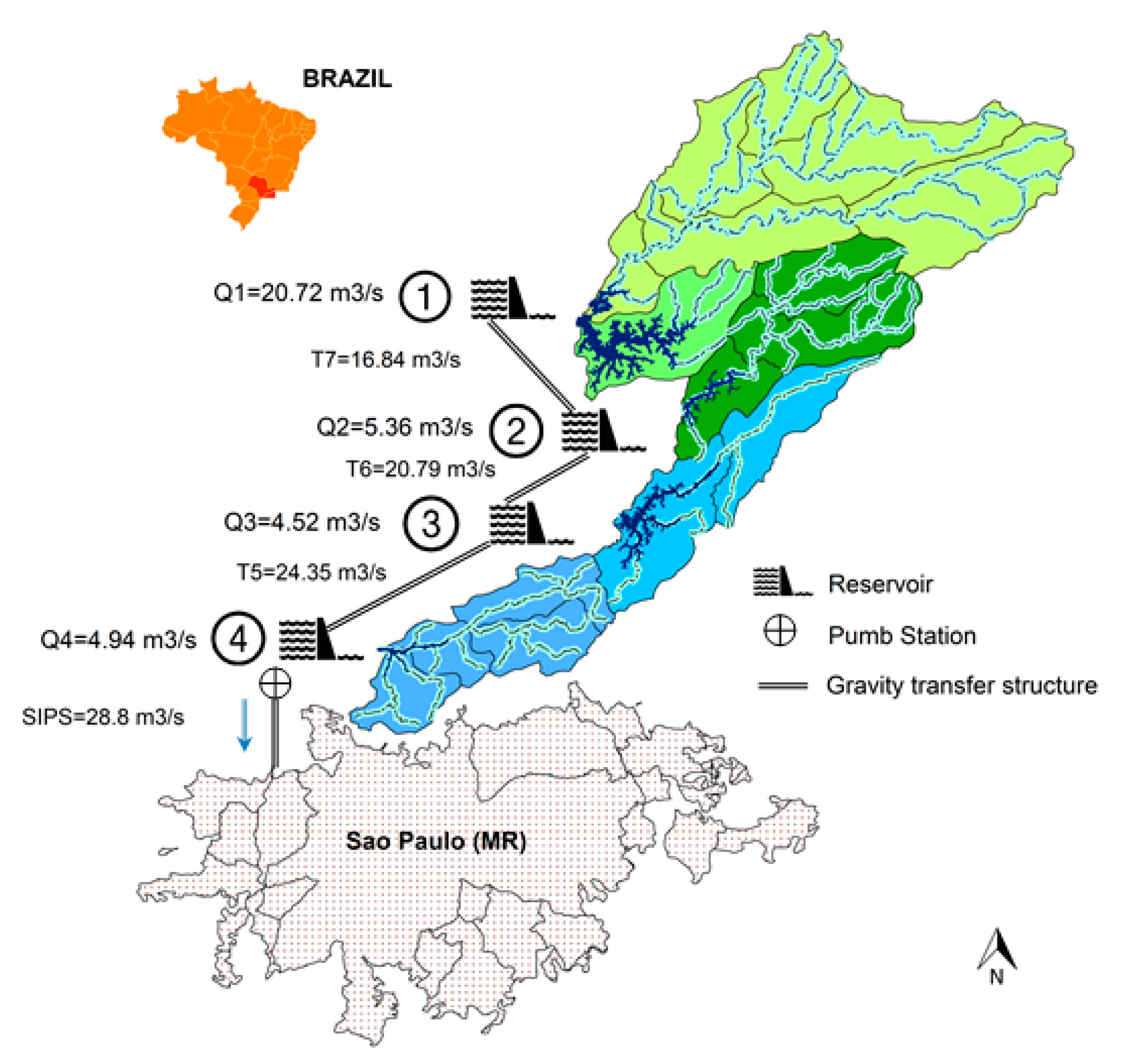
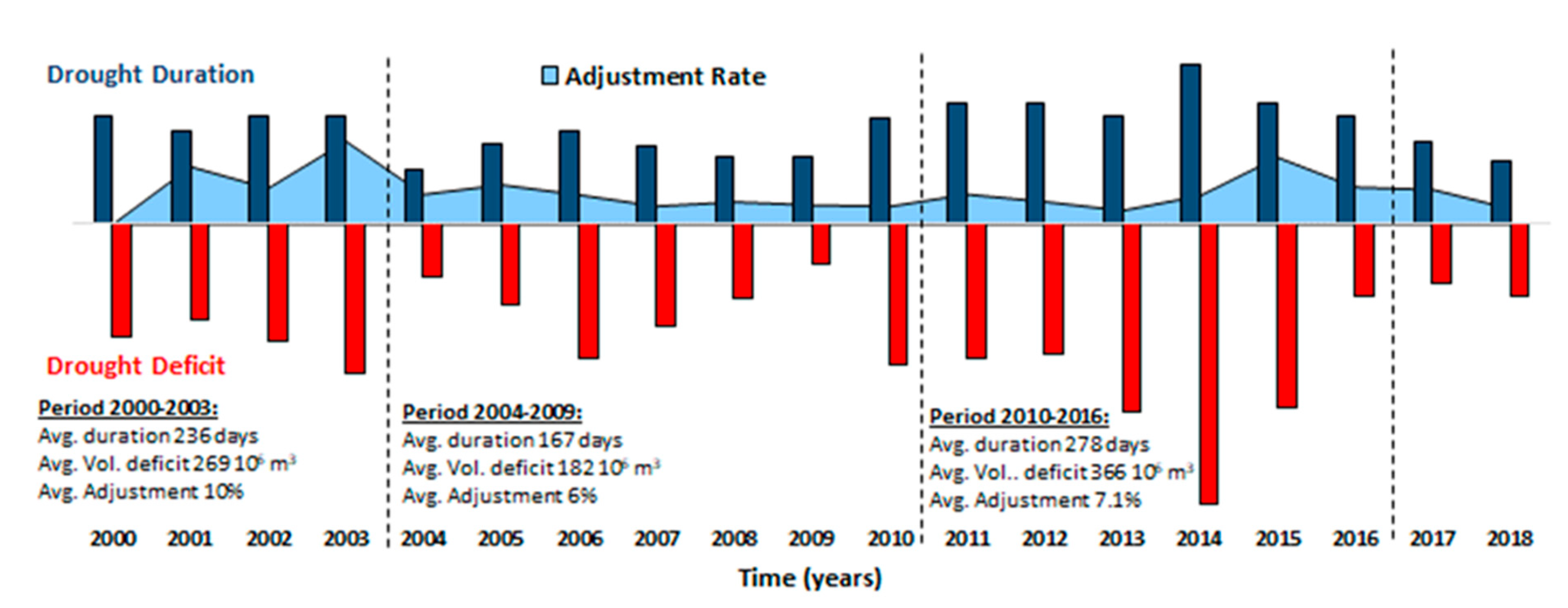
2. Study Area and Water Utility Financial Crisis Context

The SPMR, located in the State of Sao Paulo in southeast Brazil with a population of over 21 million people, is considered the fourth-largest urban agglomeration in the world. Accounting for approximately 10% of the Brazilian population according to Instituto Brasileiro de Geografia e Estatistica (IBGE), its gross domestic product (GDP) represents almost 19% of the national economy [20]. To supply the growing demand for water in the urban and industrial center, the Cantareira water supply system operation has gradually been introduced since the mid-20th century. The system currently has estimated water withdrawal of 28.8 m³·s⁻¹ to supply nine million people in the SPMR [21].

The system consists of four interconnected major reservoirs installed in four sub-watersheds of the Piracicaba River (Jaguarí–Jacareí, Cachoeira, Atibainha, and Paiva Castro) and a pumping station (see Figure 1). The Jaguarí–Jacareí sub-basins account for approximately 58% of the total water produced in the Cantareira, a percentage close to the total water withdrawn for the SPMR [21]. The water withdrawn by the SABESP for the SPMR supply system is mainly distributed for human consumption (domestic use), followed by industrial and agricultural production [22].

In recent decades, some drought events were recorded in the SPMR [23], but there were none like the 2013–2015 event that caused a water crisis with severe socioeconomic impacts in the region [24]. The event, characterized by rainfall anomalies during 2012–2015 in southeastern Brazil [9], resulted in a severe water deficit in 2014 and 2015 [25]. Throughout the deficit period, it was necessary to implement contingency measures such as rationing and water policy prices to control water consumption. The reduced water availability and price policies had consequences for water utilities, such as partial or total business interruption [26,27]. For example, the 2017 SABESP administrative report showed the net margin and net profits before, during, and after the drought period of 2012–2017 (see

Table 1. Sao Paulo Water Utility Company (SABESP) net margin and net profits under the last drought condition scenario [12,28].

Index	2012 (Before)	2013 (During)	2014 (During)	2015 (During)	2016 (After)	2017 (After)
Net margin (%)	17.8	17.0	8.1	4.6	20.9	17.2
Net profit (106 USD) *	479.2	481.9	226.24	134.3	738.3	631.2

* Present value (Jan 2018; foreign exchange R$ to USD).

). The net margin and net profits affected by the drought showed a reduction close to 60% during 2014 and 2015. It is worth mentioning that this water deficit caused direct and indirect economic losses in other sectors, such as households, industry, and peri-urban agriculture, that are highly dependent on the water supplied by the SABESP.

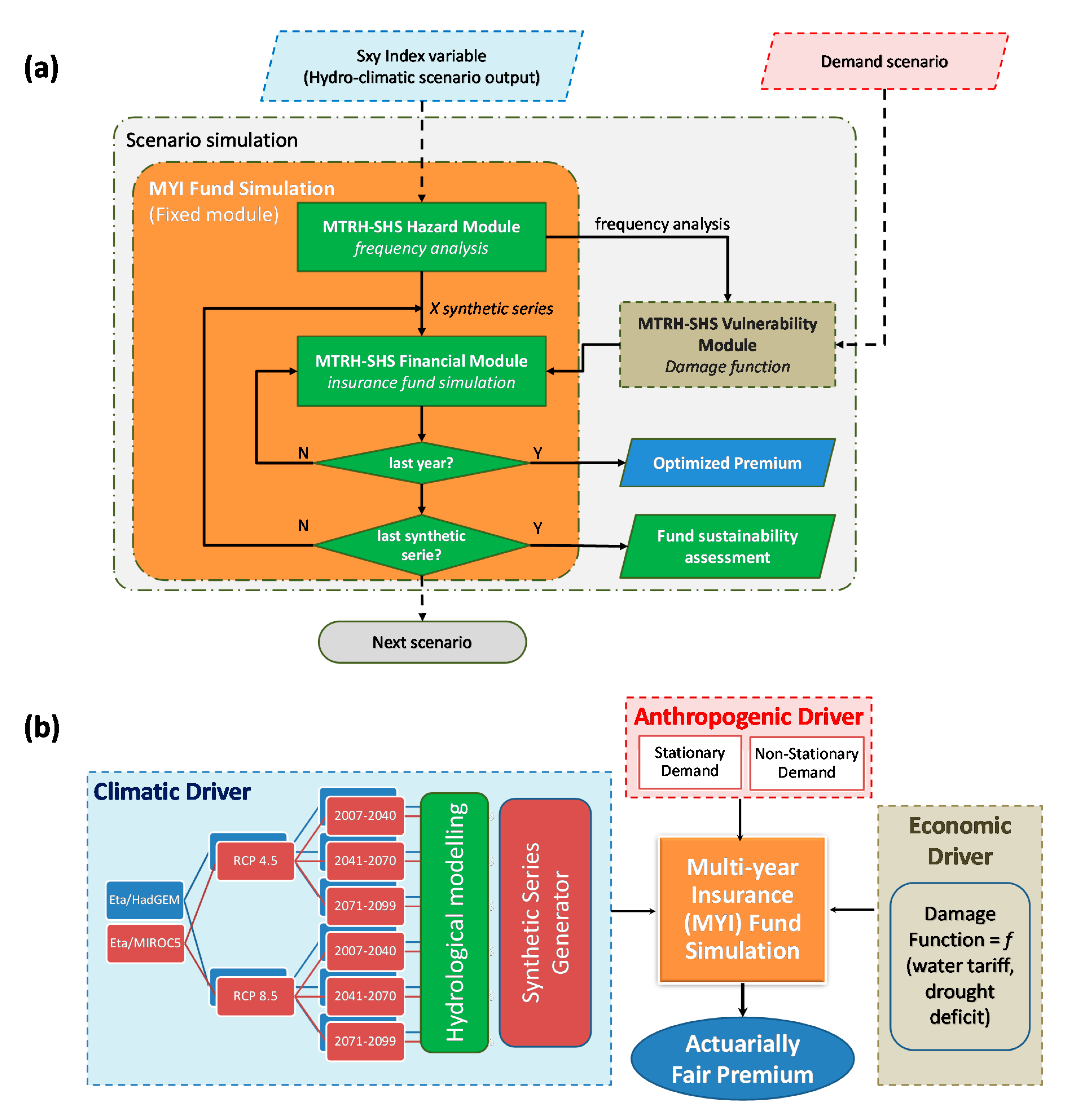
3. Materials and Methods

The framework of this application revolved around our hydrologic risk transfer model, the MTRH-SHS, which is an integrated hydrological hazard insurance fund simulation model [19]. Through sequential calculation steps, the model estimates the actuarially fair premium of a multi-year insurance contract under given scenarios.

The model structure comprises three modules (Figure 2a; detailed in Section 3.2): the hazard module, which defines and statistically describes the index variable or temporal hydrological variable under study (e.g., rainfall, water level, or drought deficit); the vulnerability module, which comprises a (set of) suitable damage function(s) (empirical or synthetic); and the financial module, which calculates the optimal insurance premium (actuarially fair premium) based on simulations of x series of the set index variable (using a synthetic generator). The model is conditioned to a multi-year contract scheme (of n years), and its financial performance is evaluated at the end of each contractual period through the loss ratio, efficiency index, and solvency index, each of which are defined in the figure below [29].

The framework was structured to simultaneously analyze the three drivers (Figure 2b), defined as follows:

First, the climatic driver, implemented in the framework through the water evaluation and planning system (WEAP), incorporates a structured hydrological model for analysis [30]. The WEAP is driven by the outputs of the RCM Eta with a grid size of 20 × 20 km and a domain over South America [31]. The Eta is nested within three global climate models (GCMs)—HadGEM2-ES, MIROC5, and BESM—used for the assessment of climate change projections in the region. Comparisons between the Eta simulations and historical observed values showed, in general, that the nested simulations represent the major features of the South America climatology and Brazil [32]. According to Chou et al. [33], Eta models nested in HADGEM2-ES presented better spatial correlations with the maximum temperature observations and mean precipitation, while those nested in MIROC5 showed better correlations with minimum temperature [33]. For this study, the projections based on Eta models HadGEM2-ES and MIROC5 forced by two representative concentration pathways (RCPs), scenarios 8.5 and 4.5, that describe pessimistic and optimistic greenhouse gas emissions, respectively, were selected [34]. The projections are given in future time slices of approximately 30 years (2007–2040, 2041–2070, and 2071–2099), adopted as multi-year insurance scheme contractual periods (defined as n). Based on the results of Chou et al. [34], although warming is projected in the entire continent, Eta model HadGEM2-ES forced by the RCP 8.5 scenario describes a larger amplitude compared to the other scenarios. While a major change in precipitation is given by reduced rain in southeast Brazil, this intensifies toward the end of the century in both emission scenarios of the Eta HadGEM simulations. Despite this reduction of precipitation, during the rainy season, heavy precipitation events become more frequent in future time slices, suggesting mixed precipitation changes in the southeast of Brazil [34].

Second, the anthropogenic driver is implemented through the variability in water demand projections. We propose a water demand scenario as stationary demand (SD), equal to 31 m³·s⁻¹, which is calculated as the average of the natural water production of the equivalent system (ES) with a 95% supply guarantee [22,28]. Another water demand scheme is defined as non-stationary demand (NSD), ranging from 31 to 36 m³·s⁻¹. The NSD was estimated as the relationship between the present population in the SPMR, the assumption of current demand for 2007–2040 (95% supply guarantee), and the demand projection as a function of population increase (IBGE database, Population Projection of Brazil and the Federation Units and Municipalities) for 2041–2070 and 2071–2099 with an 83% supply guarantee.

Third, the economic driver associates the water price policies adopted by the SABESP under the last drought period, 2013–2015 [35], to a damage function. Each simulation scenario was carried out through 100 equiprobable discharge series for each climate scenario, RCP, temporal projection, demand (SD–NSD), magnitude of drought (Rp), and insurance coverage based on Dd to finally evaluate a total of 43,500 scenarios (see Figure 2b).

We accessed several databases to feed each specific driver in MTRH-SHS processing modules (see Figure 2b). The Cantareira system soil map and land use information to define the hydrological model were adopted from [36,37]. To calibrate and validate the hydrological model’s WEAP, we used observed hydrologic data taken from HIDROWEB (the National Water Agency (ANA) database), the SABESP, and the São Paulo State Water and Electricity Department (DAEE). The dataset of climate change projections over South America was consulted through the model Eta on the Center for Weather Forecast and Climatic Studies of the Brazilian National Institute for Space Research (CPTEC/INPE) platform [38]. Finally, to define the annual increase rate variations in annual water tariffs, the SABESP’s (SABESP annual percentage increase rate 2001–2018 database) tariff readjustment and tariff cost per cubic meter of water open databases were consulted.

3.1. Risk Transfer Scheme Features

In our proposed scheme, an insurance contract will be mandatory for the water company during the three contractual periods delimited by the RCM outputs (2007–2040, 2041–2070, and 2071–2099).

Table 2. Features of adopted drought insurance design under the MTRH-SHS approach (adapted from [39]).

Feature	Description
Insurance regulations	Administration of private insurance (SUSEP) in Brazil: - National private insurance council (CNSP), Legal Resolution No. 343 of 26 December 2016 - SUSEP Circular No. 256 of 16 June 2004
Hazard approach	Hydrological drought
Insurance sector	Private insurance (disaster coverage for businesses)
Coverage (what and who)	What: Business interruption cost [26]; revenue losses related to selling water in household and industrial sectors during hydrological deficit until 100-year return period (Rp) [40,41] Who: Public services (water utility company revenue losses)
Coverage scale	Meso-scale (the Sao Paulo Metropolitan Region (SPMR)), lumped as watershed system model
Insurance planning scenarios	- Hydrological drought severity between 2-, 20-, and 100-year Rp scenarios and two water withdrawal scenarios (stationary demand–non-stationary demand (SD–NSD)) - Residual risk related to storage deficit under drought severity of 100-year Rp and two water withdrawal scenarios
Purchase requirement	Compulsory under an MYI contract scheme
Premium setting	Risk actuarially fair premium (free of administrative costs)
Hydrological variable *	Intra-annual droughts: 0 days < drought duration (Dd) < 365 days, from the monthly threshold level method (TLM) analysis
Loss function *	Empirically based curves as a function of annual maximum drought duration (days) and tariff policy price adopted during deficit periods (USD)
Insurance performance indexes	Loss ratio, efficiency, and solvency coefficients

* These features evolved from the previous version of the model by Mohor and Mendiondo [40] as follows: (a) Hydrological variable: In the former version the index variable was annual minimum 7-day streamflow, indexed by return period only; in the current version, the index variable is based on both the return period and drought duration and is developed on a monthly step; additionally, in the previous version, the index variable was fitted to a Gumbel distribution, while in the current version, values were fitted to generalized extreme value (GEV) models of all three types as the complexity of different drought durations and frequencies are considered (see Section 3.2.1). (b) Loss function: In the former version, sectoral loss functions were developed as synthetic (“what-if”) functions based on interrupted production (revenue loss) or equivalent water price (to meet water supply); in the current version, an empirical curve was developed according to observed water tariff adjustments of the water utility company.

shows descriptions of the main features adopted by the MTRH-SHS approach under the current Brazilian insurance regulations. Therefore, the premium is based on a multi-year insurance policy against risk of water shortage covering only losses by business interruption. Moreover, during a water deficit period, the insurance coverage only implies economic compensation to the water company and not the supply guarantee to user sectors. However, the company must provide the vital minimum level of water in homes and, ideally, a basic volume for industries that rely on water for their production, assuming that this can happen under a scenario of financial liquidity of the water company.

The MTRH-SHS parameters were defined as follows. First, the initial storage capital was established from the minimum solvency capital, in this case without considering assets of the insurance company. Hence, the minimum solvency capital was defined as one-third the value of the average annual loss per coverage scenario and the premium amount collected in the first period [42]. Next, loan and saving interest rates were assumed according to Central Bank of Brazil rates at 13% and 8.5% (annual percentage rate (APR)), respectively. Later, to control the high premium values during the optimization process, Graciosa [43] defined a maximum insurance fund storage limit. This value is limited to twice the loss value corresponding to the maximum hydric deficit in each simulation. Finally, it was proposed that the surplus fund, a result of hydrologically-convenient scenarios, be stored at an intermediate interest rate equal to 9% (APR).

3.2. MTRH-SHS Module Structure Descriptions

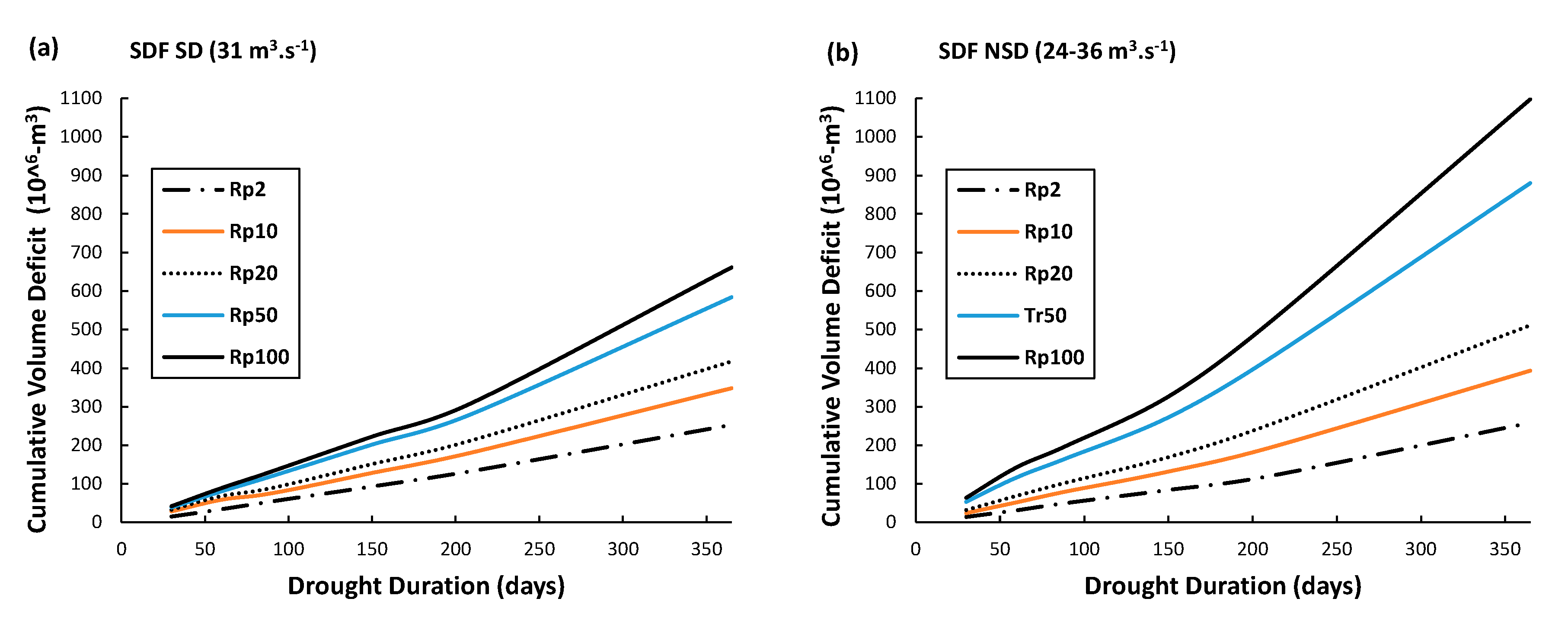
3.2.1. Hazard Module

In the event of a hydrological drought, when water demand is not controlled for or management solutions such as reservoirs are not enough, water utility companies are highly financially affected. In order to link hydrological drought with the financial impact, a hydric deficit measure was incorporated in our insurance scheme based on the traditional approaches of the threshold level method (TLM) and severity–duration–frequency (SDF) curves [44]. The SDF approach is based on the main drought characteristics under study, such as deficit and duration, to project probable events through frequency analysis [45].

Following the methodological structure based on the proposed hydrological risk transfer model, future water supply scenarios were developed through hydrological modeling with the WEAP driven by the RCM Eta outputs [46] in monthly time steps from 2004 to 2015. As criteria for model performance, we calculated the Nash–Sutcliffe efficiency index (NSE) and volumetric error in terms of percent bias (PBIAS), which presented mean values between 0.9 and 0.95 and between −12.36 and −3.4, respectively [18].

Based on the historical monthly discharge of the Cantareira system (1930–2016), a reconstructed series for the analysis of water concession authorization of the system and reservoir operation [22], and the current projected water withdrawal authorization and maximum, the SDF curves were constructed [47,48,49,50]. The SDF curves were defined from two water withdrawal assumptions (thresholds): stationary demand (SD = 31 m³·s⁻¹) and non-stationary demand (NSD = 24–36 m³·s⁻¹, gradually increasing over the period); three drought magnitude scenarios of 2-, 10-, 20-, 50-, and 100-year Rp estimated through generalized extreme value (GEV) distribution, which are widely used in studies of hydrometeorological extremes; and negative log-likelihood (maximum likelihood estimation—MLE) as a location (µ),scale (σ) and shape (ξ) parameter estimation method (see Figure 3). The SDF curves were developed from six intra-annual drought durations (30, 60, 90, 150, 210, and 365 days), and return periods of 2, 20, and 100 years were selected because these frequencies represent the envelope and central values of the intensity and duration of hydrological drought. The GEV parameters for stationary and non-stationary water withdrawal and longer droughts showed a better fit to type I or Gumbel extreme distribution functions, while shorter droughts were better adjusted to type III and II functions (Weibull and Frechet) in the stationary and non-stationary cases, respectively. The diagnostic fit plots can be reviewed in Supplementary Materials A.

3.2.2. Vulnerability Module

During the 2013–2015 drought in the SPMR, reactive economic contingencies were implemented, such as increased water tariffs, extra fees, and price incentives, all of which had a detrimental effect on the SABESP’s profit margin [12,21]. Since the SDF curves do not include the economic impact variable, characteristics such as drought duration and volume deficit can relate to water utility company revenue losses (see Figure 4). Thus, we established a drought revenue loss cost estimation based on the observed market price method [26]. For this, we developed an empirical relationship between the water price (impact) and drought duration based on the TLM [51,52,53]. Of the three observed variables of drought duration, severity, and price adjustment rates, we took drought duration as an indicator of water pricing, given that severity is always controlled by reservoirs and the transfer system (see Supplementary Materials A, Figure S1).

Three price adjustment vs. drought duration scenarios were established. The first was 100% water availability. In this scenario, the reservoir network is not essential to ensure water supply (drought duration between 0 and 90 days). The second was water availability with supply warranty and dependence on the storage system. In this scenario, the reservoir network provides resilience during droughts of smaller magnitude and duration (between 90 and 180 days). The third was stored water shortage and forced interruption of supply. In this scenario, the water deficit prevails, along with extra fees and other saving measures (drought duration between 180 and 365 days) (see Supplementary Materials B, Figure S4).

Since a water price formation study was not part of this work because it entails a complex microeconomic analysis [54], we adopted the average price of water [55] in the SPMR for the domestic and industrial sectors based on average price of USD 3.38 per m³ in 2018, assuming that this value considers normal supply conditions or 100% water availability. During the most severe droughts, an increase in the water tariff for the following period is expected. When smaller deficits are overcome with the water stored in the system, the increase in tariffs is a consequence of the annual Consumer Price Index (CPI) and other tariff updates according to the law [55].

From the cumulative drought duration intervals in SDF curves and three annual tariff adjustment classes (minimum 6% to maximum 17%), the water prices were established, as shown in

Table 3. Main assumptions for establishing tariff water price according to drought duration.

Drought Duration (Days) *	Water Tariff Adjustment Adopted (%)	Average Price (USD/m3)	Cantareira System Robustness Characteristic Scenarios
0 to 31	0	3.38	100% water availability base scenario
0 to 90	6	3.58	100% water availability
0 to 180	10	3.71	Water availability with storage dependency
0 to 365	17	3.95	Water deficit (multi-year droughts)

* Cumulative drought duration.

. Table 3 shows the inelastic behavior of the price elasticity of demand (PED), which shows closer intervals as water supplies are reduced due to drought and higher prices are imposed to try to reduce demand. Hence, a successful price-based rationing policy requires a progressive increase if the demand becomes predominantly inelastic [56], as the proposed hypothesis establishes in this case.

Based on the hydrological and economic information, empirical water utility company profit loss curves were constructed (see Figure 5). Figure 5 shows the drought duration vs. profit loss of the water utility company for different demand and return period scenarios. The damage curves were constructed by considering the priority supply to the household sector, with the industrial sector supplied once household consumption is satisfied. According to Brazilian law, the domestic sector has priority in the water supply; therefore, the predominance of dark bars shows that, to a greater extent, the economic impact comes from the industrial sector. The dark and dotted bars represent the average percentage of the economic effect of the water utility company for the industrial and household sectors, respectively, as estimated from water that was not billed by the consumption sectors.

3.2.3. Financial Module

The insurance financial simulation continued with the mean monthly flow equiprobable series generator by the method of Thomas and Fiering [57]. The method reproduced the original monthly discharges generated in the WEAP from assembling the climate and RCP baseline modelled scenarios. Next, the systematic analysis of each equiprobable series was carried out under the assumption of stationary and non-stationary water demand using the TLM [58], which calculates the difference between supply and demand. This calculation could result in an accumulated water deficit or supply guarantee during the analyzed period. Finally, the relationship between deficit, drought duration, and profit loss was assessed by the drought profit loss curves.

Thus, the actuarially fair premium P_x,N,y was calculated through annual step simulations from the balance storage in Equation (1), the optimization function (OF) in Equation (2), and a restriction:

$$S{A}_i=S{A}_{i-1}\left(1+t_{x1}\right)+p_i-I_i-L_i\left(1+t_{x2}\right)-{\left[A{t}_i\right]}^{*}+{\left[d_i\right]}^{*}$$

(1)

$$OF=min\left(S{A}_{nf}\right)$$

(2)

Restricted to accumulate loans L in the last period n_f, L_nf = 0. In Equation (1), SA_i is the fund storage in period i, t_x1 and t_x2 are the interest rates, p_i is the annual premium added, I_i is the indemnification or paid claims per period, L_i is the loans, At_i (concerning surtaxes imposed on the risk premium, SUSEP in Brazil, as a simplified case, suggests 10% as an administrative fee, 15% for brokerage commission, and 5% for profit [59]) is administrative taxes, d_i is the deductible ([At_i]^* and [d_i]^* are optional variables), and n_f is the final step of the contractual period.

Finally, we propose that the actuarially fair premium is calculated according to Equation (3) [56,60,61,62]:

$${\mathrm{Actuarially}\mathrm{Fair}\mathrm{Premium}}_{x,y}={\overline{P}}_{x,N,y}·\left(1-{\left(1-\frac{{\overline{C}}_{x,N,y}}{{\overline{TC}}_{x,N}}\right)}^n\right)$$

(3)

where x is the evaluation scenario under the set of drivers, N refers to the total evaluated equiprobable series, y is the drought duration scenario, and n is the number of years adopted in the contract. Furthermore, $\overline{P}$_x,N,y is the average expected actuarially fair premium, $\overline{C}$_x,N,y is the projected average number of paid claims per drought duration scenario y, and $\overline{TC}$_x,N,y is the total projected average claims per scenario x. The relationship between $\overline{C}$_x,N,y and $\overline{TC}$_x,N,y can be defined as the claim’s probability p during the successive years covered by the contract.

In order to define the actuarially fair premium with a certain level of confidence, the model estimates the ambiguity α associated with actuarially fair premium dispersion per scenario [14,17,59]. In this case, alpha was the variation coefficient, which allowed us to compare the differences between scenarios, since the average premiums will always be positive. Equation (4) shows how the actuarially fair premium ambiguity can be measured:

$${\mathrm{Risk}\mathrm{Premium}}_{x,y}^{*}={\mathrm{Risk}\mathrm{Premium}}_{x,y}·\left(1\pm {\alpha }_{\delta }\right)$$

(4)

where the asterisk (*) denotes the risk premium related to the ambiguity and α_δ is the ambiguity range (or premium uncertainty) associated with the scenario ($\delta$) drivers.

Three insurance performance indices were evaluated as the financial module outputs: loss ratio, solvency coefficient, and efficiency coefficient. The loss ratio (LR) is the ratio between paid claim summations and total collected premiums (Equation (5)). This index evaluates the relationship between the average amounts of premiums collected (${\overline{TEP}}_{x,N,y}$), which is used to cover the average claims (${\overline{PC}}_{x,N,y}$) during the contractual coverage period. Therefore, an LR value close to the unit represents a low profit level and an unattractive scheme for insurers [63].

$$L{R}_{x,y}= \left(\frac{{{\displaystyle \sum }}_1^n{\overline{PC}}_{x,N,y}}{{{\displaystyle \sum }}_1^n{\overline{TEP}}_{x,N,y}}\right)$$

(5)

To complement the LR evaluation, the solvency coefficient SC (Equation (6)), adapted by Laurentis [41], and the efficiency coefficient EC (Equation (7)), as previously defined by Graciosa [42], were adopted. The SC index assesses the insurance fund’s capacity to cover its financial commitments—in this case, through the initial defined capital and the annually collected premiums. The EC index appraises the probability of occurrence of a favorable scenario [41].

$$S{C}_{x,y}= \frac{Risk Premiu{m}_{x,y}-{\overline{C}}_{x,N,y}}{{\overline{C}}_{x,N,y}}$$

(6)

$$E{C}_{x,y}= \frac{TE{S}_{x,N,y}}{T{S}_{x,N,y}}$$

(7)

where $TE{S}_{x,N,y}$ is the total number of efficient series in each scenario (x and y) in the N generated equiprobable series. The TES calculation is defined by the account expression $\left({\overline{P}}_{x,N,y}-P_{x,N,y}\right)>0$, with $P_{x,N,y}$ as each expected actuarially fair premium. Likewise, $T{S}_{x,N,y}$ is the total of N evaluated series. Therefore, the index results will be better for higher EC values, i.e., there is more likely to be a favorable scenario for the insurance implementation. Finally, this index is mostly influenced by RCM projections and the covered risk magnitude.

4. Results

4.1. Actuarially Fair Premiums

The results are shown as a set of average premiums under the multi-year contract scheme that considers the drivers of change (climate, anthropogenic, and economic) analyzed in the MTRH-SHS simulation. Each drought insurance coverage set consisted of a combination of 24 driver scenarios, each one assessed from 100 equiprobable series. Figure 6 shows boxplots of average premiums for each time period vs. different insurance coverages, i.e., contracts that cover all drought durations (short and long), partial coverage, or contracts that exclusively cover long durations.

It was expected that a wider coverage level (i.e., coverage of low-duration droughts, Dd > 0, or longer droughts, Dd > 120 days or more) would lead to higher premiums compared with coverage that is restricted to events with a lower recurrence probability (i.e., longer durations, Dd > 300 days). In this way, the premium magnitude increases with the greater frequency of claims or the greater coverage of the insurance fund, a relationship that led to the final compensation paid in our model (see Figure 6). The largest boxes can be observed in the climate scenarios for 2007–2040 and 2071–2099, while the period of 2041–2070 shows the lowest average and dispersion of premium values.

In general, premiums based on the Eta-MIROC 4.5 model outputs showed higher average values than the other implemented climate scenarios, especially for the range of drought coverage of 0 or 180 days onwards, while the Eta-HadGEM 8.5 model outputs showed the lowest values for the coverage range. Throughout the simulated time periods, the results showed that premium values based on NSD, RCM Eta/MIROC, RCP 4.5, and 100-year Rp presented greater magnitudes. On the other hand, for drought duration coverage over 300 days (extreme), it was not possible to establish a significant difference in the average premium values between the evaluated scenarios, even when considering the Rp drought magnitude scenario (see Supplementary Materials C).

Though there was no clear trend in average precipitation in the Eta future projections, the annual cycle of precipitation showed that the Eta simulations driven by MIROC5 produced more precipitation than that driven by HadGEM2-ES during the rainy season and generally less during the dry season [33], which may explain the trend toward higher insurance premium values for the simulated scenarios under this climate model.

Based on the administrative and financial report of the SABESP [12], the average net profit of the company before (2012) and after (2016) the drought was USD 759 million dollars per year; however, from 2013 to 2015 (during the drought period), this average liquid net value lowered to USD 350 million per year (see Table 1). This suggests a revenue reduction of approximately USD 409 million per year for the water utility company. Based on these loss values, it would be convenient for the company to contract a multi-year insurance scheme with premiums below the average revenue reductions.

Table 4. Insurance scheme results under main analysis drivers.

Hydroclimatological Scenario x	Avg. Annual Premium (106 USD)	Demand Scenarios (%) *	Avg. Annual Premium (GDP %) **	Potential Annual Bonus Discount (106 USD)	Avg. Loans (106 USD)
Rp 100–365 > 0, 2007–2099   SD–NSD
4.5 Eta/MIROC5	938–1636	42	0.27–0.47	268–1133	20–43
4.5 Eta/HadGEM	779–1362	43	0.22–0.40	161–1044	70–127
8.5 Eta/MIROC5	889–1408	37	0.25–0.42	405–1408	8–49
8.5 Eta/HadGEM	701–1128	38	0.20–0.33	141–479	26–149
Rp 100–365 > 180, 2007–2099   SD–NSD
4.5 Eta/MIROC5	578–1198	52	0.16–0.35	27–86	204–517
4.5 Eta/HadGEM	378–980	61	0.11–0.29	2–208	310–551
8.5 Eta/MIROC5	458–951	51	0.13–0.28	9–137	289–666
8.5 Eta/HadGEM	356–570	38	0.11–0.16	3–14	342–520
Rp 100–365 > 300, 2007–2099   SD–NSD
4.5 Eta/MIROC5	21–110	81	0.005–0.04	0–0	99–315
4.5 Eta/HadGEM	36–269	87	0.01–0.07	0–3.5	131–593
8.5 Eta/MIROC5	9–82	89	0.002–0.02	0–0.3	51–244
8.5 Eta/HadGEM	29–93	69	0.009–0.02	0–0	117–275
Rp 2–365 > 0, 2007–2099   SD–NSD
4.5 Eta/MIROC5	427–584	27	0.13–0.16	117–394	10–14
4.5 Eta/HadGEM	352–484	27	0.10–0.14	59–497	35–46
8.5 Eta/MIROC5	403–505	20	0.11–0.15	185–560	3–17
8.5 Eta/HadGEM	316–409	23	0.09–0.11	47–231	13–48
Rp 2–365 > 180, 2007–2099   SD–NSD
4.5 Eta/MIROC5	269–425	38	0.07–0.13	8–48	100–186
4.5 Eta/HadGEM	176–345	49	0.05–0.11	0.4–71	150–202
8.5 Eta/MIROC5	212–338	37	0.06–0.09	2–87	133–239
8.5 Eta/HadGEM	166–203	18	0.04–0.05	1.2–8	158–181
Rp 2–365 > 300, 2007–2099   SD–NSD
4.5 Eta/MIROC5	10–38	74	0.002–0.011	0–0	48–109
4.5 Eta/HadGEM	18–92	80	0.005–0.02	0–1.2	63–203
8.5 Eta/MIROC5	5–28	82	0.0015–0.009	0–0.1	25–83
8.5 Eta/HadGEM	14–32	56	0.004–0.010	0–0	56–94

* Premium difference between stationary and non-stationary interval demand scenarios in column 2. ** Average premium as % of Sao Paulo Metropolitan Region GDP, 2016.

shows the average annual risk premium and other important results of the proposed insurance scheme scenarios, where it is clear that extensive coverage against drought events is financially unsustainable. These results suggest a financial convenience of insurance coverage for only the most unlikely events, which in this case may be droughts lasting longer than 240 days. Among the other results shown in Table 4, we found the average difference between stationary and non-stationary water demand scenarios, as presented in column 3, which are shown to increase as insurance coverage decreases to less frequent events of longer duration. Column 4 shows the average annual risk premium based on the SPMR’s gross domestic product in 2016, with the clarification that in this case, only the profit loss from the company’s losses were considered and other SPMR economical representative sectors were not. Finally, columns 5 and 6 show the potential discount on the annual risk premium value and the average loans the insurance fund would have to resort to in case of illiquidity, respectively. These characteristics of the insurance fund showed that the higher the premium, the higher the discount and the lower the loans. However, coverage only for greater magnitude drought events was found to show different loan behavior, since the average loans were reduced in such cases, probably indicating better convergence in the premium optimization process.

4.2. Premium Ambiguity

To estimate the uncertainty degree associated with insurance simulation, we analyzed insurance premium ambiguity across the coverage contracts and time slices. Figure 7 shows the average risk premium, represented by a solid line, and the range of variation that the average insurance premium could have for each simulated time period (2007–2099) and contract coverage event (Dd), represented by dashed lines. The results confirmed that insurance coverage only for the residual risk of most unlikely events has a lower ambiguity grade, while broader insurance coverage to protect against a broader range of drought durations can be economically unfavorable due to the high cost of premiums [27]. On the one hand, the ambiguity values were also found to be relatively lower and more stable during the projected period of 2041–2070 for drought coverage longer than 180 days compared with the results for 2007–2040 and 2071–2099. On the other hand, during the period of 2071–2099, the longest drought events showed higher ambiguity and insurance premium values than the other periods, possibly because the Eta simulations driven by HadGEM2-ES and MIROC5 intensified the reduction of precipitation toward the end of the century [33].

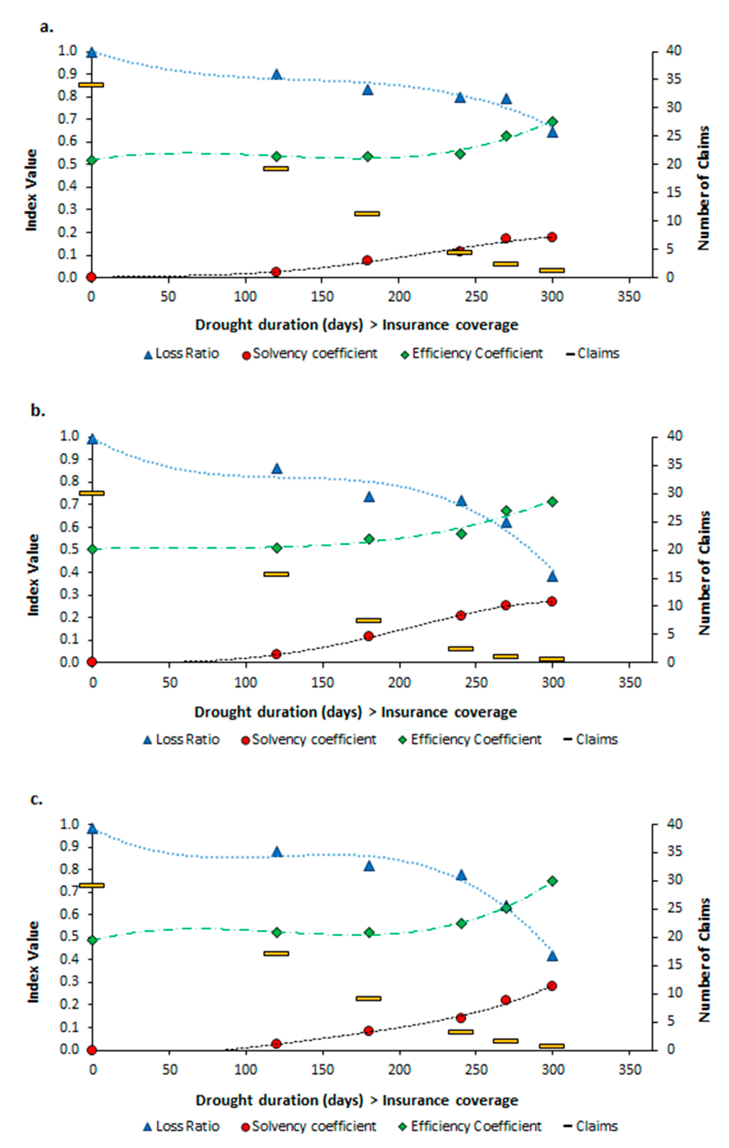
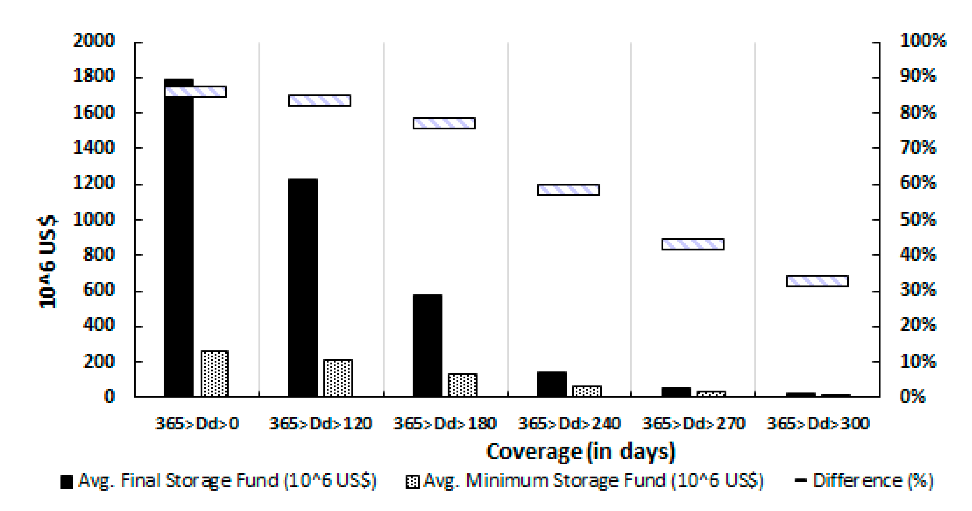
4.3. Insurance Fund Performance Indices

In order to have a comprehensive view of the insurance fund performance in each projected period, the EC, SC, and LR indicators and the number of claims were evaluated. Figure 8 shows the average value of each index as a function of insurance coverage through the analyzed scenarios. Based on the estimated LR, used to measure the economic stability of the insurance fund economic (the lower the value of LR, the greater the financial sustainability) [63,64], it was found that for less probable event coverage, the LR index line showed an inflection point that favored the collection of premiums and paid indemnities of events that recur less (Dd > 300 days). In the same way as LR, the efficiency and solvency coefficients showed improved performance under exclusive coverage conditions of greater magnitude events that consequently presented fewer claims during the contractual period.

Based on the insurance fund optimization function, defined as the minimization of the final step stored balance SA_nf (see Section 3.2.3), a comparison was made between SA_nf and the minimum solvency capital required (MSCR) for the fund’s subsistence (see Figure 9). The difference between SA_nf and MSCR offers a measure of the premium optimization process, shown by as a percentage by the semi-bar in Figure 9. On the one hand, higher differences denote premiums capable of responding to fund obligations with extremely high premiums due to the sequence of claims for the wide event coverage. On the other hand, smaller differences can be explained as better convergence to the optimal premium in response to scenarios with better claims distribution over time that facilitate the optimization process. Therefore, it is not the objective to ensure coverage close to 100% of drought risk; instead, the objective should be to only transfer the risk of greater magnitude and have less probability of occurrence.

5. Discussions and Conclusions

In this paper, we proposed a multi-year insurance scheme to face the revenue losses of a water utility company during hydric deficit periods that, in recent years, have intensified in the SPMR. The insurance scheme was based on the MTRH-SHS methodology, executed mainly under the influence of climate and water-demand drivers. The approach describes how the proposed drivers influence the annual risk premium value from the medium to long term. Additionally, based on the obtained results, a premium ambiguity measure was estimated, and this is useful for defining pricing policies in the insurance sector and business interruption risk planning.

This study, besides attempting to contribute to insurance design planning, attempted to assess the impacts of climate change in different economic sectors on a regional scale. In addition, pessimistic and optimistic RCP scenarios and the Eta downscaling technique of two global models provided more possibilities and further addressed uncertainties in assessing hydrological insurance premiums.

Regarding the proposed insurance scheme results, it can be concluded that contracts for exclusive coverage of more unlikely events (that is, more severe and prolonged events), despite showing high ambiguity, present more promising financial conditions than contracts for broader coverage and thus represent an important alternative for water service companies.

On the other hand, this study shows the need to evaluate the residual risk of reservoirs that assume the risk for low-to-medium drought and should be supplemented with insurance strategies in the future. This was mainly proposed with the aim of configuring an efficient management strategy that considers the current dynamics of risk.

Indeed, these advances are valuable, especially for communicating risk insurance in developing and transitional economies, like those of some South American, African, and Asian countries, with a significant variety of factors like exposure, hazard, and vulnerability. Addressing that, violin plots (see Supplementary Materials C) show the amplitude of responses of our MYI–SDF methodology. The violin plots show how the decision-making process of choosing climate models, demand intervals, hazard ranges, and planning periods affects water risk averse premiums and potential affordability for vulnerable sectors and utilities under uncertain change scenarios.

Moreover, this version of MYI introduces distinctive advances for drought risk aversion, with theoretical and applied backgrounds that link donor basins (supply) and metropolitan water utilities (demand). This scaling condition is a spatially-distinctive boundary condition that can be flexibly adapted to other cases worldwide.

In the absence of precise information on the drought impact in different water supply sectors, the information on revenue losses due to SABESP business interruptions was used because the dataset could show a lower degree of uncertainty when the damage costs were evaluated. This implies that there needs to be an effort to collect, process, and make available useful information for varied purposes.

Alternatively, the stored surplus fund could be invested in risk-reduction strategies [65] or used to finance ecosystem services to guarantee water security. However, given the difficulty in translating such strategies into actual loss reduction at either the individual or public levels, as well as the subjectivity to know whether there could be political will to implement such strategy for the latter, this alternative scenario will be studied in future work.

This study offers a methodological foundation for further studies using recent advances in drought insurance. First, the paper shows a portable methodology for how MYI premiums, from changing drivers, might influence water users’ demand for insurance if SDF curves are included. Thus, MYI could establish new risk-averse functions (expanding the work of Leblois et al. [66]) and elicit a long-run capacity to adapt to climate change when subsidized and non-subsidized water markets are envisaged [67].

It can be concluded, based on the SABESP’s recent annual revenue losses and the average risk premium calculated here, that it would be convenient to acquire insurance to cover the economic impacts of hydrological drought in the SPMR, especially given the hypothetical market capability to offer the depicted insurance policy. Finally, the evaluation of the insurance scheme under a new driver configuration, such as longer-term multi-annual insurance contracts and the introduction of various deductible schemes, is open for future analysis.

References

1. Pichs-Madruga, Y.; Sokona, E.; Farahani, S.; Kadner, K.; Seyboth, A.; Adler, I.; Baum, S.; Brunner, P.; Eickemeier, B.; Kriemann, J.; et al. IPCC, 2014: Summary for Policymakers. In Climate Change 2014: Mitigation of Climate Change. Contribution of Working Group III to the Fifth Assessment Report of the Intergovernmental Panel on Climate Change; Cambridge University Press: Cambridge, UK; New York, NY, USA, 2014. [Google Scholar]
2. WMO. Atlas of Mortality and Economic Losses from Weather, Climate and Water Extremes; Publications Board World Meteorological Organization (WMO): Geneva, Switzerland, 2014; ISBN 978-92-63-11123-4. [Google Scholar]
3. Di Giulio, G.M.; Bedran-Martins, A.M.B.; Vasconcellos, M.D.P.; Ribeiro, W.C.; Lemos, M.C. Mainstreaming climate adaptation in the megacity of São Paulo, Brazil. Cities 2017, 72, 237–244. [Google Scholar] [CrossRef]
4. Huang, S.; Li, P.; Huang, Q.; Leng, G.; Hou, B.; Ma, L. The propagation from meteorological to hydrological drought and its potential influence factors. J. Hydrol. 2017, 547, 184–195. [Google Scholar] [CrossRef]
5. Wu, J.; Chen, X.; Yao, H.; Gao, L.; Chen, Y.; Liu, M. Non-linear relationship of hydrological drought responding to meteorological drought and impact of a large reservoir. J. Hydrol. 2017, 551, 495–507. [Google Scholar] [CrossRef]
6. Stahl, K.; Kohn, I.; Blauhut, V.; Urquijo, J.; De Stefano, L.; Acacio, V.; Dias, S.; Stagge, J.H.; Tallaksen, L.M.; Kampragou, E.; et al. Impacts of European drought events: Insights from an international database of text-based reports. Nat. Hazards Earth Syst. Sci. 2016, 16, 801–819. [Google Scholar] [CrossRef] [Green Version]
7. Schäfer, L.; Waters, E.; Kreft, S.; Zissener, M. Making Climate Risk Insurance Work for the Most Vulnerable: Seven Guiding Principles; United Nations University Institute for Environment and Human Security: Bonn, Germany, 2016. [Google Scholar]
8. Mello, K.; Randhir, T. Diagnosis of water crises in the metropolitan area of São Paulo: Policy opportunities for sustainability. Urban Water J. 2017, 15, 53–60. [Google Scholar] [CrossRef]
9. Nobre, C.A.; Marengo, J.A. Water Crises and Megacities in Brazil: Meteorological Context of the São Paulo Drought of 2014–2015; Global Water Forum: Brasilia, Brazil, 2016. [Google Scholar]
10. Soriano, E.; Torres, L.; Gregorio, D.I.; Coutinho, M.P.; Bacellar, L.; Santos, L. Water Crisis in Sao Paulo Evaluated Under the Disaster’s point of view. Ambient. Soc. 2016, 19, 21–42. [Google Scholar] [CrossRef] [Green Version]
11. Empinotti, V.L.; Budds, J.; Aversa, M. Governance and water security: The role of the water institutional framework in the 2013–15 water crisis in São Paulo, Brazil. Geoforum 2019, 98, 46–54. [Google Scholar] [CrossRef] [Green Version]
12. GESP. Relatório da Administração 2016—Companhia de Saneamento Básico do Estado de São Paulo—SABESP; Report: Companhia de Saneamento Básico do Estado de São Paulo—SABESP; SABESP: Sao Paulo, Brazil, 2016. [Google Scholar]
13. Doncaster, C.P.; Tavoni, A.; Dyke, J.G. Using Adaptation Insurance to Incentivize Climate-change Mitigation. Ecol. Econ. 2017, 135, 246–258. [Google Scholar] [CrossRef]
14. Kunreuther, H.; Michel-Kerjan, E. Economics of Natural Catastrophe Risk Insurance. In Handbooks in Economics: Economics of Risk and Uncertainty; Machina, M.J., Viscusi, K.W., Eds.; Elsevier: Amsterdam, The Netherlands, 2014; pp. 651–699. ISBN 9780444536853. [Google Scholar]
15. Savitt, A. Insurance as a tool for hazard risk management? An evaluation of the literature. Nat. Hazards 2017, 86, 583–599. [Google Scholar] [CrossRef]
16. Daron, J.D.; Stainforth, D.A. Assessing pricing assumptions for weather index insurance in a changing climate. Clim. Risk Manag. 2014, 1, 76–91. [Google Scholar] [CrossRef] [Green Version]
17. Zhu, W. A model of catastrophe risk pricing and its empirical test School of Finance. Insur. Math. Econ. 2017, 77, 14–23. [Google Scholar] [CrossRef]
18. Guzman, D.A. Hydrological Risk Transfer Planning under the Drought “Severity-Duration-Frequency” Approach as a Climate Change Impact Mitigation Strategy; Sao Paulu Univeristy: Sao Paulo, Brazil, 2018. [Google Scholar]
19. Mohor, G.S.; Mendiondo, E.M. Economic indicators of hydrologic drought insurance under water demand and climate change scenarios in a Brazilian context. Ecol. Econ. 2017, 140, 66–78. [Google Scholar] [CrossRef]
20. Haddad, E.A.; Teixeira, E. Economic impacts of natural disasters in megacities: The case of floods in Sao Paulo, Brazil. Habitat Int. 2015, 45, 106–113. [Google Scholar] [CrossRef] [Green Version]
21. SABESP. Sistema Cantareira. Available online: http://www2.ana.gov.br/Paginas/servicos/saladesituacao/v2/SistemaCantareira.aspx (accessed on 31 December 2016).
22. ANA; DAEE. Subsídios Para a Análise do Pedido de Outorga do Sistema Cantareira e Para a Definição das Condições de Operação dos Seus Reservatórios; ANA/DAEE Technical Note: Estado de São Paulo, Brazil, 2004. [Google Scholar]
23. Nobre, C.A.; Marengo, J.A.; Seluchi, M.E.; Cuartas, A.; Alves, L.M. Some Characteristics and Impacts of the Drought and Water Crisis in Southeastern Brazil during 2014 and 2015. J. Water Resour. Prot. 2016, 8, 252–262. [Google Scholar] [CrossRef] [Green Version]
24. Milano, M.; Reynard, E.; Muniz-miranda, G.; Guerrin, J. Water Supply Basins of São Paulo Metropolitan Region: Hydro-Climatic Characteristics of the 2013–2015 Water Crisis. Water 2018, 10, 1517. [Google Scholar] [CrossRef] [Green Version]
25. Taffarello, D.; Samprogna Mohor, G.; do Carmo Calijuri, M.; Mendiondo, E.M. Field investigations of the 2013–14 drought through quali-quantitative freshwater monitoring at the headwaters of the Cantareira System, Brazil. Water Int. 2016, 8060, 1–25. [Google Scholar] [CrossRef]
26. Meyer, V.; Becker, N.; Markantonis, V.; Schwarze, R.; Van Den Bergh, J.C.J.M.; Bouwer, L.M.; Bubeck, P.; Ciavola, P.; Genovese, E.; Green, C.; et al. Review article: Assessing the costs of natural hazards-state of the art and knowledge gaps. Nat. Hazards Earth Syst. Sci. 2013, 13, 1351–1373. [Google Scholar] [CrossRef]
27. Zeff, H.B.; Characklis, G.W. Managing water utility financial risks through third-party index insurance contracts. Water Resour. Res. 2013, 49, 4939–4951. [Google Scholar] [CrossRef]
28. SABESP. Relatório da Administração 2017; Technical Note; SABESP: Sao Paulo, Brazil, 2017. [Google Scholar]
29. Mohor, G.S. Seguros Hídricos como Mecanismos de Adaptação às Mudanças do Clima para Otimizar a Outorga de Uso da Água. Master’s Thesis, Sao Paulo University, Sao Paulo, Brazil, 2016. [Google Scholar]
30. World Bank. Lesotho WEAP Manual; License: Creative Commons Attribution CC BY 3.0 IGO; World Bank: Washington, DC, USA, 2017. [Google Scholar]
31. Dereczynski, C.; Chan Chou, S.; Lyra, A.; Sondermann, M.; Regoto, P.; Tavares, P.; Chagas, D.; Gomes, J.L.; Rodrigues, D.C.; Skansi, M.d.l.M. Downscaling of climate extremes over South America—Part I: Model evaluation in the reference climate. Weather Clim. Extrem. 2020, 29, 100273. [Google Scholar] [CrossRef]
32. Almagro, A.; Oliveira, P.T.S.; Rosolem, R.; Hagemann, S.; Nobre, C.A. Performance evaluation of Eta/HadGEM2-ES and Eta/MIROC5 precipitation simulations over Brazil. Atmos. Res. 2020, 244, 105053. [Google Scholar] [CrossRef]
33. Chou, S.C.; Lyra, A.; Mourão, C.; Dereczynski, C.; Pilotto, I.; Gomes, J.; Bustamante, J.; Tavares, P.; Silva, A.; Rodrigues, D.; et al. Evaluation of the Eta Simulations Nested in Three Global Climate Models. Am. J. Clim. Chang. 2014, 3, 438–454. [Google Scholar] [CrossRef] [Green Version]
34. Chou, S.C.; Lyra, A.; Mourão, C.; Dereczynski, C.; Pilotto, I.; Gomes, J.; Bustamante, J.; Tavares, P.; Silva, A.; Rodrigues, D.; et al. Assessment of Climate Change over South America under RCP 4.5 and 8.5 Downscaling Scenarios. Am. J. Clim. Chang. 2014, 3, 512–527. [Google Scholar] [CrossRef] [Green Version]
35. SABESP. COMUNICADO—03/16: Marco Tarifario RMSP. 2016. Available online: http://site.sabesp.com.br/site/uploads/file/clientes_servicos/comunicado_03_2016.pdf (accessed on 1 August 2017).
36. De Oliveira, J.B.; Camargo, M.; Rossi, M.; Filho, B.C. Mapa Pedológico do Estado de São Paulo, 1st ed.; Embrapa, IAC: Campinas, Brazil, 1999; ISBN 8585564032. [Google Scholar]
37. Molin, P.G.; Miranda, F.T.S.; Sampaio, J.V.; Fransozi, A.A.; Ferraz, S.D.B. Mapeamento de uso e Cobertura do Solo da Bacia do Rio Piracicaba, SP: Anos 1990, 2000 e 2010; Technical Report no. 207; Circular Tecnica/Instituto de Pesquisas e Estudos Florestais: Sao Paulo, Brazil, 2015. [Google Scholar]
38. Holbig, C.A.; Mazzonetto, A.; Borella, F.; Pavan, W.; Fernandes, J.M.C.; Chagas, D.J.; Gomes, J.L.; Chou, S.C. PROJETA platform: Accessing high resolution climate change projections over Central and South America using the Eta model. Agrometeoros 2019, 26, 7. [Google Scholar] [CrossRef]
39. UNISDR. Insurance Development Forum: Defining the Protection Gap “Working Group on Metrics & Indicators”. Available online: https://www.unisdr.org/files/globalplatform/591d4fcfd34e8Defining_the_Protection_Gap_Working_Paper.pdf (accessed on 1 December 2016).
40. Surminski, S.; Bouwer, L.M.; Linnerooth-Bayer, J. How insurance can support climate resilience. Nat. Clim. Chang. 2016, 6, 333–334. [Google Scholar] [CrossRef] [Green Version]
41. Paudel, Y.; Botzen, W.J.W.; Aerts, J.C.J.H.; Dijkstra, T.K. Risk allocation in a public—Private catastrophe insurance system: An actuarial analysis of deductibles, stop-loss, and premiums. J. Flood Risk Manag. 2015, 8, 116–134. [Google Scholar] [CrossRef]
42. Laurentis, G.L. de Modelo De Transferência De Riscos Hidrológicos Como Estratégia De Adaptação Às Mudanças Globais Segundo Cenários De Vulnerabilidade Dos Recursos Hídricos. Master’s Thesis, Escola de Engenharia de São Carlos, Sao Paulo, Brazil, 2012. [Google Scholar]
43. Graciosa, M.C. Modelo de Seguro Para Riscos Hidrológicos com Base em Simulação Hidráulico-Hidrológica como Ferramenta Para Gestão do Risco de Inundações. Ph.D. Thesis, University of São Paulo, Sao Paulo, Brazil, 2010. [Google Scholar]
44. Sung, J.H.; Chung, E.S. Development of streamflow drought severity-duration-frequency curves using the threshold level method. Hydrol. Earth Syst. Sci. 2014, 18, 3341–3351. [Google Scholar] [CrossRef] [Green Version]
45. Dalezios, N.R.; Loukas, A.; Vasiliades, L. Severity-duration-frequency analysis of droughts and wet periods in Greece. Hydrol. Sci. J. 2000, 45, 751–769. [Google Scholar] [CrossRef]
46. Santos, C.A.S.; Rocha, F.A.; Ramos, T.B.; Alves, L.M.; Mateus, M.; de Oliveira, R.P.; Neves, R. Using a hydrologic model to assess the performance of regional climate models in a semi-arid Watershed in Brazil. Water 2019, 11, 170. [Google Scholar] [CrossRef] [Green Version]
47. Firoz, A.B.M.; Nauditt, A.; Fink, M.; Ribbe, L. Quantifying human impacts on hydrological drought using a combined modelling approach in a tropical river basin in Central Vietnam. Hydrol. Earth Syst. Sci. 2018, 22, 547–565. [Google Scholar] [CrossRef] [Green Version]
48. Tallaksen, L.M.; Madsen, H.; Clausen, B. On the definition and modelling of streamflow drought duration and deficit volume. Hydrol. Sci. J. 1997, 42, 15–33. [Google Scholar] [CrossRef]
49. Zaidman, M.D.; Keller, V.; Young, A.R.; Cadman, D. Flow-duration-frequency behaviour of British rivers based on annual minima data. J. Hydrol. 2003, 277, 195–213. [Google Scholar] [CrossRef]
50. Rojas, L.P.T.; Díaz-Granados, M. The construction and comparison of regional drought severity-duration-frequency curves in two Colombian River basins-study of the Sumapaz and Lebrija Basins. Water 2018, 10, 1453. [Google Scholar] [CrossRef] [Green Version]
51. Bachmair, S.; Kohn, I.; Stahl, K. Exploring the link between drought indicators and impacts. Nat. Hazards Earth Syst. Sci. 2015, 15, 1381–1397. [Google Scholar] [CrossRef] [Green Version]
52. Hou, W.; Chen, Z.Q.; Zuo, D.D.; Feng, G. lin Drought loss assessment model for southwest China based on a hyperbolic tangent function. Int. J. Disaster Risk Reduct. 2018, 33, 477–484. [Google Scholar] [CrossRef]
53. Mens, M.J.P.; Gilroy, K.; Williams, D. Developing system robustness analysis for drought risk management: An application on a water supply reservoir. Nat. Hazards Earth Syst. Sci. 2015, 15, 1933–1940. [Google Scholar] [CrossRef] [Green Version]
54. Garrido, R. Price Setting for Water Use Charges in Brazil Price Setting for Water Use Charges in Brazil. Int. J. Water Resour. Dev. 2005, 21, 99–117. [Google Scholar] [CrossRef]
55. SABESP. Regulamento do Sistema Tarifário da Sabesp. Available online: http://site.sabesp.com.br/site/interna/Default.aspx?secaoId=183 (accessed on 1 December 2018).
56. Mays, L.W.; Tung, Y.-K. Economics for Hydrosystems. In Hydrosystemas Engineering and Management; McGraw-Hill: New York, NY, USA, 2002; pp. 23–50. [Google Scholar]
57. Vaghela, C.R.; Vaghela, A.R. Synthetic Flow Generation. Int. J. Eng. Res. Apl. 2014, 4, 66–71. [Google Scholar]
58. Hisdal, H.; Tallaksen, L.M.; Clausen, B.; Peters, E.; Gustard, A. Hydrological Drought Characteristics. In Developments in Water Science: Hydrological Drought, Processes and Estimation Methods for Streamflow and Groundwater; Tallaksen, L.M., Van Lanen, H.A.J., Eds.; Elsevier: Amsterdam, The Netherlands, 2004; pp. 139–198. ISBN 0-444-51767-7. [Google Scholar]
59. SUSEP. Como é Calculado o Prêmio de Seguro? Available online: http://www.susep.gov.br/setores-susep/cgpro/coseb (accessed on 1 August 2017).
60. Kunreuther, H.; Pauly, M.V.; McMorrow, S. Insurance & Behavioral Economics: Improving Desicions in the Most Misunderstood Industry, 1st ed.; Cambridge University Press: New York, NY, USA, 2013; ISBN 9781107013445. [Google Scholar]
61. Kunreuther, H.; Useem, M. Learning Fromm Catastrophes: Strategies for Reaction and Response, 1st ed.; Wharton School Publishing: Upper Saddle River, NJ, USA, 2010; ISBN 9780137044856. [Google Scholar]
62. Şen, Z. Applied Drought Modeling, Prediction, and Mitigation; Şen, Z., Ed.; Elsevier: Amsterdam, The Netherlands, 2015; ISBN 9780128021767. [Google Scholar]
63. Dionne, G. Risk Sharing and Pricing in the Reinsurance Market, 2nd ed.; Dionne, G., Ed.; Springer: Montreal, QC, Canada, 2013; ISBN 9781461401551. [Google Scholar]
64. Contador, C.R. Economia do Seguro: Fundamentos e Aplicações, 1st ed.; Atlas: Sao Paulo, Brazil, 2007; ISBN 8522448108. [Google Scholar]
65. Hudson, P.; Botzen, W.J.W.; Feyen, L.; Aerts, J.C.J.H. Incentivising flood risk adaptation through risk based insurance premiums: Trade-offs between affordability and risk reduction. Ecol. Econ. 2016, 125, 1–13. [Google Scholar] [CrossRef]
66. Leblois, A.; Le Cotty, T.; Maître d’Hôtel, E. How Might Climate Change Influence farmers’ Demand for Index-Based Insurance? Ecol. Econ. 2020, 176, 106716. [Google Scholar] [CrossRef]
67. Miao, R. Climate, insurance and innovation: The case of drought and innovations in drought-tolerant traits in US agriculture. Eur. Rev. Agric. Econ. 2020, 1–35. [Google Scholar] [CrossRef]
Figure 1. Cantareira water supply system: 1: Jaguarí–Jacareí subsystem; 2: Cachoeira subsystem; 3: Atibainha subsystem; and 4: Paiva Castro subsystem. Qx, daily average discharge of subsystem x, 2004–2016; Ty, daily average water withdrawal of tunnel y, 2004–2016; and SIPS, Santa Isabel Pump Station.
Water 12 02954 g001
Figure 2. (a) Methodology flowchart linked to multi-year insurance (MYI) Modelo de Transferência de Riscos Hidrológicos of the Department of Hydraulics and Sanitation at Sao Paulo University (MTRH-SHS) fund simulator: climatic driver related to hydrological modeling, anthropogenic driver related to demand scenarios, economic driver related to tariff cost readjustment; (b) MTRH-SHS general application and module connections. Sxy, index variable, e.g., streamflow or processed variable as water deficit.
Water 12 02954 g002
Figure 3. Severity–duration–frequency (SDF) curves under SD and NSD demand assumptions in reconstructed discharge scenarios for 1930–2016: (a) SD = 31 m3·s−1; (b) NSD = 24–36 m3·s−1.
Water 12 02954 g003
Figure 4. Empirical relationship between Cantareira system drought duration (blue bars, in days), derived from monthly average discharge analysis, drought deficit (red bars, in 106 m3), and annual price adjustment rates under variable hydrological conditions (in percentages).
Water 12 02954 g004
Figure 5. Relationships of profit loss derived from 360-day continuous drought per sector—industrial (Ind., continuous line) and household (Hou., dashed line). From top to bottom: return period (Rp) from 100, 20, and 2 years under water demand scenarios of stationary demand (SD = 31 m3 s−1) and non-stationary demand (NSD = 24–36 m3 s−1).
Water 12 02954 g005
Figure 6. Average (dots) and range (boxplots) of actuarially fair premiums per drought duration coverage at each regional climate model (RCM) output time period: (a) 2007–2040, (b) 2041–2070, and (c) 2071–2099 while considering the set of change drivers (climate, demand, and frequency; each boxplot comprises 2400 data points).
Water 12 02954 g006
Figure 7. Average insurance premium ambiguity vs. drought duration coverage: (a) 2007–2040, (b) 2041–2070, and (c) 2071–2099.
Water 12 02954 g007aWater 12 02954 g007b
Figure 8. Performance indices of insurance scheme against hydrological drought (loss ratio, solvency coefficient, efficiency coefficient, and number of claims): (a) 2007–2040, (b) 2041–2070, and (c) 2071–2099.
Water 12 02954 g008
Figure 9. Comparison between final balance stored SAnf (solid bars) and average minimum storage, initially defined as minimum solvency capital (dotted bars).
Water 12 02954 g009