Deep BLSTM-GRU Model for Monthly Rainfall Prediction: A Case Study of Simtokha, Bhutan


1
Department of IT, College of Science and Technology, Chukkha 21101, Bhutan
2
Department of Computer Science & Engineering, Indian Institute of Technology Roorkee, Uttarakhand 247667, India
3
Department of IT Engineering, Sookmyung Women’s University, Seoul 04310, Korea
*
Author to whom correspondence should be addressed.
Remote Sens. 2020, 12(19), 3174; https://doi.org/10.3390/rs12193174
Submission received: 28 August 2020
/
Revised: 20 September 2020
/
Accepted: 22 September 2020
/
Published: 28 September 2020
Abstract
:Rainfall prediction is an important task due to the dependence of many people on it, especially in the agriculture sector. Prediction is difficult and even more complex due to the dynamic nature of rainfalls. In this study, we carry out monthly rainfall prediction over Simtokha a region in the capital of Bhutan, Thimphu. The rainfall data were obtained from the National Center of Hydrology and Meteorology Department (NCHM) of Bhutan. We study the predictive capability with Linear Regression, Multi-Layer Perceptron (MLP), Convolutional Neural Network (CNN), Long Short Term Memory (LSTM), Gated Recurrent Unit (GRU), and Bidirectional Long Short Term Memory (BLSTM) based on the parameters recorded by the automatic weather station in the region. Furthermore, this paper proposes a BLSTM-GRU based model which outperforms the existing machine and deep learning models. From the six different existing models under study, LSTM recorded the best Mean Square Error (MSE) score of 0.0128. The proposed BLSTM-GRU model outperformed LSTM by 41.1% with a MSE score of 0.0075. Experimental results are encouraging and suggest that the proposed model can achieve lower MSE in rainfall prediction systems.
1. Introduction
Rainfall prediction has a widespread impact ranging from farmers in agriculture sectors to tourists planning their vacation. Moreover, the accurate prediction of rainfall can be used in early warning systems for floods [1] and an effective tool for water resource management [2]. Despite being of paramount use, the prediction of rainfall or any climatic conditions is extremely complex. Rainfall depends on various dependent parameters like humidity, wind speed, temperate, etc., which vary from one geographic location to another; hence, one model developed for a location may not fit for another region as effectively. Generally, rainfall can be predicted using two approaches. The first is by studying all the physical processes of rainfall and modeling it to mimic a climatic condition. However, the problem with this approach is that the rainfall depends on numerous complex atmospheric processes which vary both in space and time. The second approach is using pattern recognition. These algorithms are decision tree, k-nearest neighbor, and rule-based methods. For a large dataset, deep learning techniques are used to find meaningful results, and these techniques are based on the neural network. In this method, we ignore the physical laws governing the rainfall process and predict rainfall patterns based on their features. This study aims to use pattern recognition to predict precipitation. The predictive models developed in this study are based on deep learning techniques. We propose a Bidirectional Long Short Term Memory (BLSTM) and Gated Recurrent Unit (GRU)-based approach for monthly prediction and compare its results with the state-of-the-art models in deep learning.
In this study, we predict rainfall over Simtokha, a region in the capital of Bhutan, Thimphu [3]. Although much work has been done on rainfall prediction using Artificial Neural Network (ANN) [4,5,6,7,8], particularly Multi-Layer Perceptron (MLP) in different countries, there is no existing literature on the application of ANN or Deep Neural Network (DNN) for the same purpose for any of the regions in Bhutan. Weather parameters vary from region to region, and the parameters recorded also vary according to the weather stations. A model developed for one country or region does not fit for another location as effectively.
The particular area was chosen as it is located in the capital of the country and serves as the primary station for the entire Thimphu. The region, although not prone to flooding, faces constant water shortages due to ineffective water resource management. A more accurate beforehand knowledge of precipitation for the coming month will help the region to identify and mitigate water shortage problems. This work also studies the predictive capability of different DNNs for predicting rainfall based on the parameters recorded by the weather stations in the country and will serve as a baseline study. The dataset used in the study is the automatic weather station data collected from a station located in Simtokha.
Atmospheric models [9] are predominantly used for forecasting rainfall in Bhutan. Atmospheric models include atmospheric circulation models, climate models, and numerical models which simulate atmospheric operation and predict rainfall. Currently, Numeric Weather Prediction (NWP) methods are the principal mode of forecasting rainfall in Bhutan. Numerical models employ a set of partial differential equations for the prediction of many atmospheric variables such as temperature, pressure, wind, and rainfall. The forecaster based on his experience examines how the features predicted by the computer will interact to produce the day’s weather.
This work focuses on the current state-of-the-art deep learning techniques to forecast rainfall over Simtokha. The contribution of our work is as follows:
- We proposed a hybrid framework of BLSTM and GRU for rainfall prediction.
- No prior deep learning techniques have been used on the dataset. The results of this paper will serve as the baseline for future researchers.
- A detailed analysis of the proposed framework is presented through extensive experiments.
- Finally, a comparison with different deep learning models is also discussed.
The rest of the paper is organized as follows. In Section 2, we discuss the existing research work in the rainfall prediction system. In Section 3, the proposed system implemented on the dataset is discussed. Section 4 describes the experimental results and analysis. Finally, in the last Section 5 the work is concluded along with a discussion of some future possibilities.
2. Literature Review
Prediction methods have come a long way, from relying on an individual’s experience to simple numeric methods to complex atmospheric models. Although machine learning algorithms like Artificial Neural Network (ANN) have been utilized by researchers to forecast rainfall, studies on the effectiveness of existing deep learning models are limited, especially on data recorded by the sensors in a weather station. Forecasting of rainfall can be conducted over a short time, such as predicting an hour or a day into the future, or over a long time such as monthly or a year ahead. A Neural Network (NN) is a collection of neurons and multiple hidden layers, which work similar to a human brain. NNs are used to classify things and are based on the data. Recent surveys [4,5,10] show MLP as the most popular NN used for rainfall prediction.
Huang et al. [11] used 4 years of hourly data from 75 rain gauge stations in Bangkok and developed a NN to forecast 1–6 h rainfall on this data. Luk et al. [12] performed short-term (15 min) prediction using data collected from 16 gauges over the catchment area in western Sydney. Both research works recommended MLP over k-nearest neighbor, multivariate adaptive regression splines, linear regression, and support vector regression. The study also highlighted the drop in prediction capability with an increase in lag order. Kashiwao et al. [13] compared MLP with an algorithm composed of random optimization, backpropagation, and Radial Bias Function Network (RBFN) to predict short-term rainfall on the data collected by the Japan Meteorological Agency (JMA). The authors showed MLP performed better than RBFN.
Hernandez et al. [14] used a combination of autoencoder and MLP to predict the amount of rainfall for the next day using previous days’ records. The autoencoder was used to extract nonlinear dependencies of the data. Their method outperformed other naive methods but had little improvement over MLP. Khajure et al. [15] used an NN and a fuzzy inference system. The weather parameters were predicted using an NN, and the predicted values were fed into the fuzzy inference system, which then predicted the rainfall according to predefined fuzzy inference system rules. The authors concluded that a fuzzy inference system can be used along with an NN to achieve good prediction results. The effectiveness of a fuzzy inference system for rainfall prediction was also reported by Wahyuni et al. [16].
Predicting monthly rainfall using MLP has shown more stable results compared to short-term prediction. Mishra et al. [17] used a feed-forward neural network (FFNN) to predict monthly rainfall over North India. Abhishek et al. [4] predicted monsoon precipitation for the Udupi district of Karnataka using three different learning algorithms: Back Propagation Algorithm (BPA), Layer Recurrent Network (LRN), and Cascaded Back Propagation (CBP). The BPA showed lower mean squared error (MSE) compared to the other algorithms. Hardwinarto et al. [18] showed a promising result of BPNN for monthly rainfall using data from Tenggarong Station in Indonesia. Kumar and Tyagi [19] found RBFN outperformed BPNN while predicting rainfall for the Coonoor region of Tamil Nadu.
With the advancement in deep learning techniques, research work has been done to implement it in time series prediction. Recurrent neural networks (RNNs), in particular LSTM [20] and GRU [21], have found their niche in time series prediction. Zaytar et al. [22] used multi-stacked LSTM to forecast 24 h and 72 h of weather data, i.e., temperature, wind speed, and humidity. They used 15 years of hourly meteorological data from 2000–2015 of nine cities of Morocco. The authors deduced deep LSTM networks could forecast the weather parameters effectively and suggested it for other weather-related problems. Salan et al. [23] used weather datasets from 1973 to 2009 provided by the Indonesian Agency for Meteorology, Climatology, and Geophysics to predict rainfall. The authors used a recurrent neural network for prediction and obtained an accuracy score of 84.8%. Qie et al. [24] used multi-task CNN to predict short-term precipitation using weather parameters collected from multiple rain gauges in China. The authors concluded that the multi-site [25] features gave better results than single-site features. A summary of the literature review is shown in Table 1.
3. Proposed System
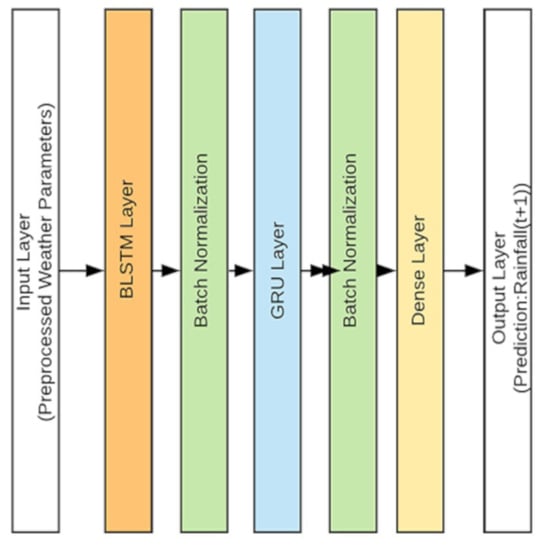
In this section, we describe the different steps and components of the proposed system. The proposed deep learning model consists of a BLSTM, GRU, and Dense layer as shown in Figure 1.
3.1. Dataset Description
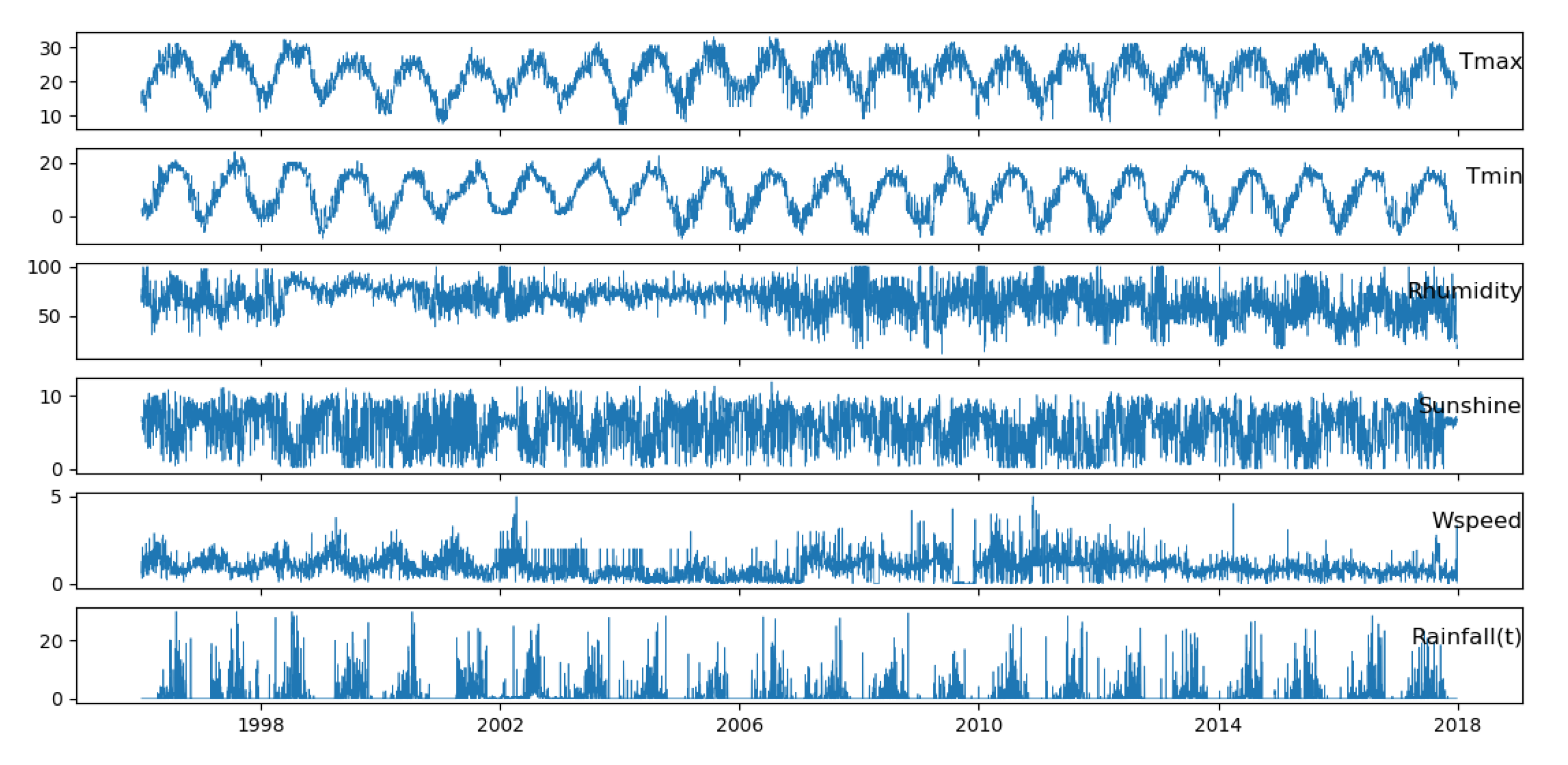
Bhutan is a small Himalayan country landlocked between India to the south and China to the north, as shown in Figure 2. The sensor data used in this work were collected from a weather station located in Simtokha [3], Thimphu, which is the 4th highest capital in the world by altitude, and the range varies from 2248 to 2648 m. The station at Simtokha is the sole station to record class A data for the capital. The station is located at 89.7 longitude and 27.4 latitude at an elevation of 2310 m. The data for this study were obtained from NCHM (http://www.hydromet.gov.bt), which provides two classes of data to researchers: class A and class C datasets. Class A datasets are recorded by automatic weather stations, and class C datasets are recorded manually by designated employees at different stations. Class A datasets are, hence, more reliable and were used in this work. The selected dataset contains daily records of weather parameters from 1997 to 2017, as shown in Figure 3. The records from 1997–2015 were used to train the different models, and 2016–2017 data were used for testing. Six weather parameters described in Table 2 were used for this study. These parameters had either zero or very few missing values that were handled during data preprocessing. The monthly weather parameters were extracted from daily records by taking the mean of tmax, tmin, relative_humidity, wind_speed, and wind_direction. The number of sunshine hours and rainfall amount in a month were deduced by taking the sum of daily sunshine hours and daily rainfall values, respectively.
3.2. Data Preprocessing
The daily records of weather parameters from 1997 to 2017 were collected from NCHM. The raw data originally contained eight parameters, but some of the parameters contained a lot of missing and noisy values. The weather parameters that contained a lot of empty records were dropped from the dataset. The dataset also had different random representations for the null value, which was standardized during preprocessing. The preprocessing step is as shown in Figure 4. The missing values in the selected parameters were resolved by taking the mean of all the values occurring for that particular day and month. For example, if the sunshine_hours record for 1 January 2000 was missing, it was filled by the mean of other sunshine_hours records on 1 January for other years. Outliers are records that significantly differ from other observed values. The outliers were detected using a box-and-whisker plot as well as the k-means clustering algorithm [26] and were resolved using the mean technique. Weather parameters were normalized using a min-max scaler to get the new scaled value z.
where min(x) and max(x) are the minimum and maximum value, respectively. x is the value to be scaled. After preprocessing, the data are reshaped into a tensor format for DNN models. The input for the LSTM layer must have a 3D shape. The three dimensions of the input are samples, time steps, and sample dimension. One sequence is considered as one sample, one point of observation in the sample is one time step, and one feature is a single point of observation at the time step. In our experiment one sample is made up of 12 time steps (12 months), and in each time step (month) there are parameters like average maximum temperature, average sunshine hours, etc.
3.3. Evaluation Metrics
The study used both qualitative and quantitative metrics to calculate the performance of different models. The formulae for RMSE, MSE, Pearson Correlation Coefficient, and were used as a scoring function, as in Table 3.
From the above, is the model simulated monthly rainfall, is the observed monthly rainfall, and are their arithmetic mean, and n is the number of data points.
3.4. BLSTM
LSTM is the most popular model in time series analysis, and there are many variants such as unidirectional LSTM and BLSTM. For our study, the Many-to-One (multiple input and one output) variation of LSTM [27,28] was used to take the last 12 months’ weather parameters and predict the rainfall for the next month, as shown in Figure 5. Unidirectional LSTM process data are based on only past information. Bidirectional LSTM [29,30,31,32,33] utilizes the most out of the data by going through time-steps in both forward and backward directions. It duplicates the first recurrent network in the architecture to get two layers side by side. It passes the input, as it is to the first layer and provides a reversed copy to the second layer. Although it was traditionally developed for speech recognition, its use has been extended to achieve better performance from LSTM in multiple domains [34,35]. An architecture consisting of two hidden layers with 64 neurons in the first layer and 32 neurons in the second layer recorded the best result on the test dataset, with MSE value of 0.01, a coefficient value of 0.87, and value of 0.75.
3.5. GRU
The Gated Recurrent Unit was developed by Cho et al. [21] in 2014. GRU performances on certain tasks of natural language processing, speech signal modeling, and music modeling are similar to the LSTM model. The GRU model has fewer gates compared to LSTM and has been found to outperform LSTM when dealing with smaller datasets. To solve the vanishing gradient problem of a standard RNN, GRU consists of an update and reset gate, but unlike the LSTM it lacks a dedicated output gate. The update gate decides how much of the previous memory to keep, and the reset gate determines how to combine the previous memory with the new input. Due to fewer gates, they are computationally less demanding compared to LSTM and are ideal when there are limited computational resources. GRU with two hidden layers consisting of 12 neurons in the first layer and 6 neurons in the second outperformed other architectures, with an MSE score of 0.02, a correlation value of 0.83, and value of 0.66.
3.6. BLSTM-GRU Model
In this model, preprocessed weather parameters are fed into the BLSTM layer with 14 neurons. This layer reads data in both forward and backward directions and creates an appropriate embedding. Batch normalization is performed on the output of the BLSTM layer to normalize the hidden embedding before passing it to the next GRU layer. The GRU layer contains half the number of neurons as the BLSTM layer. The GRU layer has fewer cells and is able to generalize the embedding with relatively lower computation cost. The data are again batch normalized before sending to the final dense layer. The final layer has just one neuron with a linear activation function, and it outputs the predicted value of monthly rainfall for T + 1 (next month), where T is the current month.
For our study, the Many-to-One (multiple input and one output) variation of LSTM [27,28] was used to take the last 12 months’ weather parameters and predict the rainfall for the next month, as shown in Figure 5. The activation function used in both BLSTM and GRU is the default tanh function, and the optimizer used was Adam. The architecture was fixed after thoroughly hyper-tuning the parameters. Hyperparameter tuning was performed through a randomized grid search and heuristic knowledge of the programmer.
4. Experiment and Results
The models were created in python on the Jupyter notebook using Keras (https://github.com/fchollet/keras) deep learning API with Tensorflow [36] back-end. All the experiments were run for 10,000 epochs, but by using callbacks in Keras only the best weight for each test run was saved. Although 10,000 epochs were not needed most of the time, smaller architectures with few neurons took considerably more time to learn as compared to neuron-rich networks. Multiple experiments were conducted with varying architecture for each model under study. Early stopping [37] with a large patience value was used to prevent unnecessary overfitting.
4.1. Result Summary
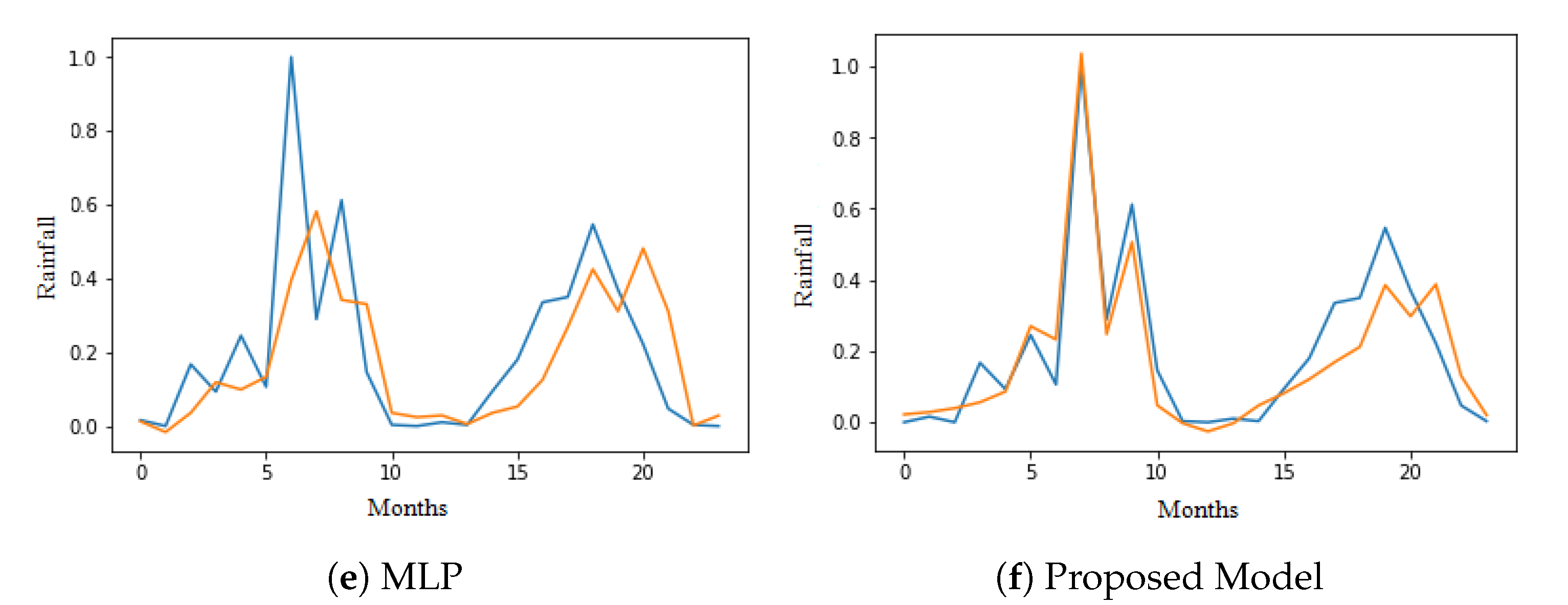
The best MSE and RMSE scores of each model are highlighted in Figure 6. The NNs outperformed linear regression by a huge margin. LSTM and GRU outperformed MLP by a huge margin, as they were able to utilize the 12 time-steps of input properly. The plots between predicted and the actual values for 24 months from January 2016 to December 2017 are shown in Figure 7.
The proposed model performed uniformly better than vanilla versions of all the deep learning techniques under study. The MSE score of 0.01 achieved by our model was 41.1% better compared to the next best score of 0.13 provided by LSTM.
4.2. Comparative Analysis
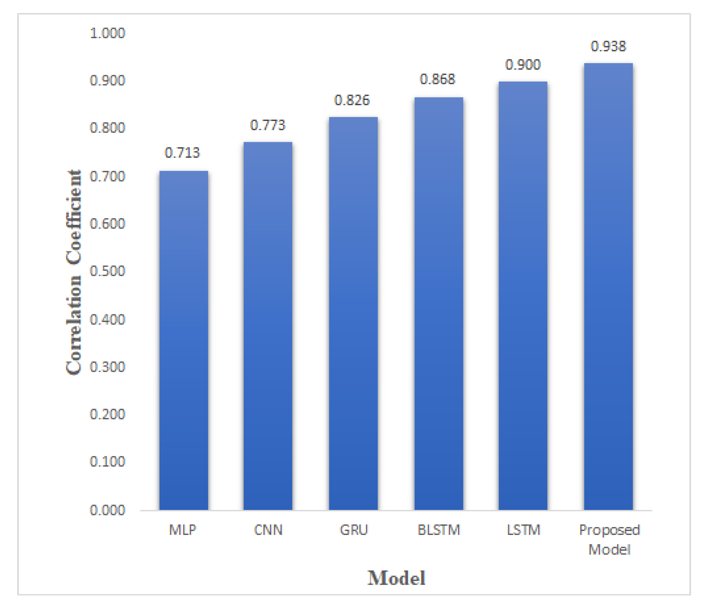
We have also compared our system with MLP, LSTM, CNN [38,39,40], and other methods on the NCHM dataset as shown in Figure 8 and Figure 9. The dataset did not have a baseline score to overcome. The linear regression RMSE score of 0.217 and MSE score of 0.047 were used as the baseline score.
Each input sample has 12 time-steps, and the output is the total amount of rainfall for the next month (t + 1). Each timestep contains the weather features of a particular month. For example, the timestep T(n) contains all the weather parameters for the nth month. From Figure 8 and Figure 9 it is evident that, among the vanilla models, LSTM with 1024 neurons performed the best with a MSE score of 0.013, a correlation value of 0.90, and value of 0.78. The proposed BLSTM-GRU model outperformed LSTM on all four performance matrices, with MSE, RMSE, , and correlation coefficient values of 0.0075, 0.087, 0.870, and 0.938 respectively.
5. Conclusions and Future Work
The study of deep learning methods for rainfall prediction is presented in this paper, and a BLSTM-GRU based model is proposed for rainfall prediction over the Simtokha region in Thimphu, Bhutan. The sensor data are collected from the meteorology department of Bhutan, which contain daily records of weather parameters from 1997 to 2017. The records from 1997–2015 are used for training machine learning and deep learning models, and for testing we used 2016–2017 data. According to sensor data, the traditional MLP (the results on the Simtokha region dataset, i.e., 0.029 MSE, 0.71 correlation, and value of 0.50), which is widely used for rainfall prediction, did not perform well in comparison to the recent deep learning models on weather station data. Vanilla versions of LSTM, GRU, BLSTM, and 1-D CNN performed similarly, with a single-layered LSTM consisting of 1024 neurons performing better than the others, with MSE score of 0.013, a correlation value of 0.90, and value of 0.78. Finally the combination of BLSTM and GRU layers performed much better than all the other models under study for this dataset. Its MSE score of 0.007 was 41.1% better than LSTM. Furthermore, the proposed model presented an improved correlation value of 0.93 and score of 0.87. Predicting actual rainfall values has become more challenging due to the changing weather patterns caused by climate change.
In the future, we aim to improve the performance of our prediction model by incorporating patterns of global and regional weather such as sea surface temperature, global wind circulation, etc. We also intend to explore the predictive use of climate indices and study the effects of climate change on rainfall patterns.
Author Contributions
All authors have contributed to this paper. M.C. proposed the main idea in consultation with P.P.R. M.C., S.K. and P.P.R. were involved in methodology and M.C. performed the experiments. M.C. and S.K. drafted the initial manuscript. P.P.R. and B.-G.K. contributed to the final version of the paper. All authors have read and agreed to the published version of the manuscript.
Funding
This research received no external funding.
Acknowledgments
The authors thank the National Center of Hydrology and Meteorology department, Bhutan, for providing the data to conduct this research.
Conflicts of Interest
The authors declare that they have no conflicts of interest in this work.
References
- Toth, E.; Brath, A.; Montanari, A. Comparison of short-term rainfall prediction models for real-time flood forecasting. J. Hydrol. 2000, 239, 132–147. [Google Scholar] [CrossRef]
- Jia, Y.; Zhao, H.; Niu, C.; Jiang, Y.; Gan, H.; Xing, Z.; Zhao, X.; Zhao, Z. A webgis-based system for rainfall-runoff prediction and real-time water resources assessment for beijing. Comput. Geosci. 2009, 35, 1517–1528. [Google Scholar] [CrossRef]
- Walcott, S.M. Thimphu. Cities 2009, 26, 158–170. [Google Scholar] [CrossRef]
- Abhishek, K.; Kumar, A.; Ranjan, R.; Kumar, S. A rainfall prediction model using artificial neural network. In Proceedings of the Control and System Graduate Research Colloquium (ICSGRC), Shah Alam, Malaysia, 16–17 July 2012; pp. 82–87. [Google Scholar]
- Darji, M.P.; Dabhi, V.K.; Prajapati, H.B. Rainfall forecasting using neural network: A survey. In Proceedings of the 2015 International Conference on Advances in Computer Engineering and Applications (ICACEA), Ghaziabad, India, 19–20 March 2015; pp. 706–713. [Google Scholar]
- Kim, J.-H.; Kim, B.; Roy, P.P.; Jeong, D.-M. Efficient facial expression recognition algorithm based on hierarchical deep neural network structure. IEEE Access 2019, 7, 41273–41285. [Google Scholar] [CrossRef]
- Mukherjee, S.; Saini, R.; Kumar, P.; Roy, P.P.; Dogra, D.P.; Kim, B.G. Fight detection in hockey videos using deep network. J. Multimed. Inf. Syst. 2017, 4, 225. [Google Scholar]
- Anh, D.T.; Dang, T.D.; Van, S.P. Improved rainfall prediction using combined pre-processing methods and feed-forward neural networks. J—Multidiscip. Sci. J. 2019, 2, 65. [Google Scholar]
- Mesinger, F.; Arakawa, A. Numerical Methods Used in Atmospheric Models; Global Atmospheric Research Program World Meteorological Organization: Geneva, Switzerland, 1976. [Google Scholar]
- Nayak, D.R.; Mahapatra, A.; Mishra, P. A survey on rainfall prediction using artificial neural network. Int. J. Comput. Appl. 2013, 72. [Google Scholar]
- Hung, N.Q.; Babel, M.S.; Weesakul, S.; Tripathi, N.K. An artificial neural network model for rainfall forecasting in bangkok, thailand. Hydrol. Earth Syst. Sci. 2009, 13, 1413–1425. [Google Scholar] [CrossRef] [Green Version]
- Luk, K.C.; Ball, J.E.; Sharma, A. An application of artificial neural networks for rainfall forecasting. Math. Comput. Model. 2001, 33, 683–693. [Google Scholar] [CrossRef]
- Kashiwao, T.; Nakayama, K.; Ando, S.; Ikeda, K.; Lee, M.; Bahadori, A. A neural network-based local rainfall prediction system using meteorological data on the internet: A case study using data from the japan meteorological agency. Appl. Soft Comput. 2017, 56, 317–330. [Google Scholar] [CrossRef]
- Hernández, E.; Sanchez-Anguix, V.; Julian, V.; Palanca, J.; Duque, A.N. Rainfall prediction: A deep learning approach. In Lecture Notes in Computer Science, Proceedings of the International Conference on Hybrid Artificial Intelligence Systems, Seville, Spain, 18–20 April 2016; Springer: Cham, Switzerland, 2016; pp. 151–162. [Google Scholar]
- Khajure, S.; Mohod, S.W. Future weather forecasting using soft computing techniques. Procedia Comput. Sci. 2016, 78, 402–407. [Google Scholar] [CrossRef] [Green Version]
- Wahyuni, I.; Mahmudy, W.F.; Iriany, A. Rainfall prediction in tengger region indonesia using tsukamoto fuzzy inference system. In Proceedings of the International Conference on Information Technology, Information Systems and Electrical Engineering (ICITISEE), Yogyakarta, Indonesia, 23–24 August 2016; pp. 130–135. [Google Scholar]
- Mishra, N.; Soni, H.K.; Sharma, S.; Upadhyay, A.K. Development and analysis of artificial neural network models for rainfall prediction by using time-series data. Int. J. Intell. Syst. Appl. 2018, 10, 16. [Google Scholar] [CrossRef]
- Hardwinarto, S.; Aipassa, M. Rainfall monthly prediction based on artificial neural network: A case study in tenggarong station, east kalimantan-indonesia. Procedia Comput. Sci. 2015, 59, 142–151. [Google Scholar]
- Kumar, A.; Tyagi, N. Comparative analysis of backpropagation and rbf neural network on monthly rainfall prediction. In Proceedings of the 2016 International Conference on Inventive Computation Technologies (ICICT), Coimbatore, India, 26–27 August 2016; Volume 1, pp. 1–6. [Google Scholar]
- Hochreiter, S.; Schmidhuber, J. Long short-term memory. Neural Comput. 1997, 9, 1735–1780. [Google Scholar] [CrossRef] [PubMed]
- Cho, K.; Van Merriënboer, B.; Gulcehre, C.; Bahdanau, D.; Bougares, F.; Schwenk, H.; Bengio, Y. Learning phrase representations using rnn encoder-decoder for statistical machine translation. arXiv 2014, arXiv:1406.1078. [Google Scholar]
- Sutskever, I.; Vinyals, O.; Le, Q.V. Sequence to sequence learning with neural networks. In Proceedings of the 2014 Neural Information Processing Systems(NIPS), Montreal, QC, Canada, 8–13 December 2014; pp. 3104–3112. [Google Scholar]
- Salman, A.G.; Kanigoro, B.; Heryadi, Y. Weather forecasting using deep learning techniques. In Proceedings of the 2015 International Conference on Advanced Computer Science and Information Systems (ICACSIS), Depok, Indonesia, 10–11 October 2015; pp. 281–285. [Google Scholar]
- Qiu, M.; Zhao, P.; Zhang, K.; Huang, J.; Shi, X.; Wang, X.; Chu, W. A short-term rainfall prediction model using multi-task convolutional neural networks. In Proceedings of the 2017 IEEE International Conference on Data Mining (ICDM), New Orleans, LA, USA, 18–21 November 2017; pp. 395–404. [Google Scholar]
- Wheater, H.S.; Isham, V.S.; Cox, D.R.; Chandler, R.E.; Kakou, A.; Northrop, P.J.; Oh, L.; Onof, C.; Rodriguez-Iturbe, I. Spatial-temporal rainfall fields: Modelling and statistical aspects. Hydrol. Earth Syst. Sci. Discuss. 2000, 4, 581–601. [Google Scholar] [CrossRef] [Green Version]
- Hartigan, J.A.; Wong, M.A. Algorithm as 136: A k-means clustering algorithm. J. R. Stat. Soc. Ser. Appl. Stat. 1979, 28, 100. [Google Scholar] [CrossRef]
- Kim, S.; Hong, S.; Joh, M.; Song, S. Deeprain: Convlstm network for precipitation prediction using multichannel radar data. arXiv 2017, arXiv:1711.02316. [Google Scholar]
- Chao, Z.; Pu, F.; Yin, Y.; Han, B.; Chen, X. Research on real-time local rainfall prediction based on mems sensors. J. Sens. 2018, 2018, 6184713. [Google Scholar] [CrossRef]
- Graves, A.; Liwicki, M.; Fernández, S.; Bertolami, R.; Bunke, H.; Schmidhuber, J. A novel connectionist system for unconstrained handwriting recognition. IEEE Trans. Pattern Anal. Mach. 2009, 31, 855–868. [Google Scholar] [CrossRef] [Green Version]
- Saini, R.; Kumar, P.; Kaur, B.; Roy, P.P.; Prosad Dogra, D.; Santosh, K.C. Kinect sensor-based interaction monitoring system using the blstm neural network in healthcare. Int. J. Mach. Learn. Cybern. 2019, 10, 2529–2540. [Google Scholar] [CrossRef]
- Mukherjee, S.; Ghosh, S.; Ghosh, S.; Kumar, P.; Pratim Roy, P. Predicting video-frames using encoder-convlstm combination. In Proceedings of the ICASSP 2019 IEEE International Conference on Acoustics, Speech and Signal Processing (ICASSP), Brighton, UK, 12–17 May 2019; pp. 2027–2031. [Google Scholar]
- Mittal, A.; Kumar, P.; Roy, P.P.; Balasubramanian, R.; Chaudhuri, B.B. A modified lstm model for continuous sign language recognition using leap motion. IEEE Sens. J. 2019, 19, 7056–7063. [Google Scholar] [CrossRef]
- Kumar, P.; Mukherjee, S.; Saini, R.; Kaushik, P.; Roy, P.P.; Dogra, D.P. Multimodal gait recognition with inertial sensor data and video using evolutionary algorithm. IEEE Trans. Fuzzy Syst. 2018, 27, 956. [Google Scholar] [CrossRef]
- Cui, Z.; Ke, R.; Wang, Y. Deep bidirectional and unidirectional lstm recurrent neural network for network-wide traffic speed prediction. arXiv 2018, arXiv:1801.02143. [Google Scholar]
- Althelaya, K.A.; El-Alfy, E.S.M.; Mohammed, S. Evaluation of bidirectional lstm for short-and long-term stock market prediction. In Proceedings of the 2018 9th International Conference on Information and Communication Systems (ICICS), Irbid, Jordan, 3–5 April 2018; pp. 151–156. [Google Scholar]
- Abadi, M.; Barham, P.; Chen, J.; Chen, Z.; Davis, A.; Dean, J.; Devin, M.; Ghemawat, S.; Irving, G.; Isard, M.; et al. Tensorflow: A system for large-scale machine learning. In Proceedings of the 12th USENIX Symposium on Operating Systems Design and Implementation OSDI, Savannah, GA, USA, 2–4 November 2016; Volume 16, pp. 265–283. [Google Scholar]
- Prechelt, L. Early stopping-but when? In Neural Networks: Tricks of the Trade; Springer: Berlin/Heidelberg, Germany, 1998; pp. 55–69. [Google Scholar]
- Kim, Y. Convolutional neural networks for sentence classification. arXiv 2014, arXiv:1408.5882. [Google Scholar]
- Yang, J.; Nguyen, M.N.; San, P.P.; Li, X.; Krishnaswamy, S. Deep convolutional neural networks on multichannel time series for human activity recognition. Ijcai 2015, 15, 3995–4001. [Google Scholar]
- Zhao, B.; Lu, H.; Chen, S.; Liu, J.; Wu, D. Convolutional neural networks for time series classification. J. Syst. Eng. Electron. 2017, 28, 162–169. [Google Scholar] [CrossRef]
Figure 1.
The proposed model is composed of 7 layers including the input and output layers. The embedding is generated by the Bidirectional Long Short Term Memory (BLSTM) and Gated Recurrent Unit (GRU) layer. The batch normalization is used for normalizing the data, and the dense layer performs the prediction.
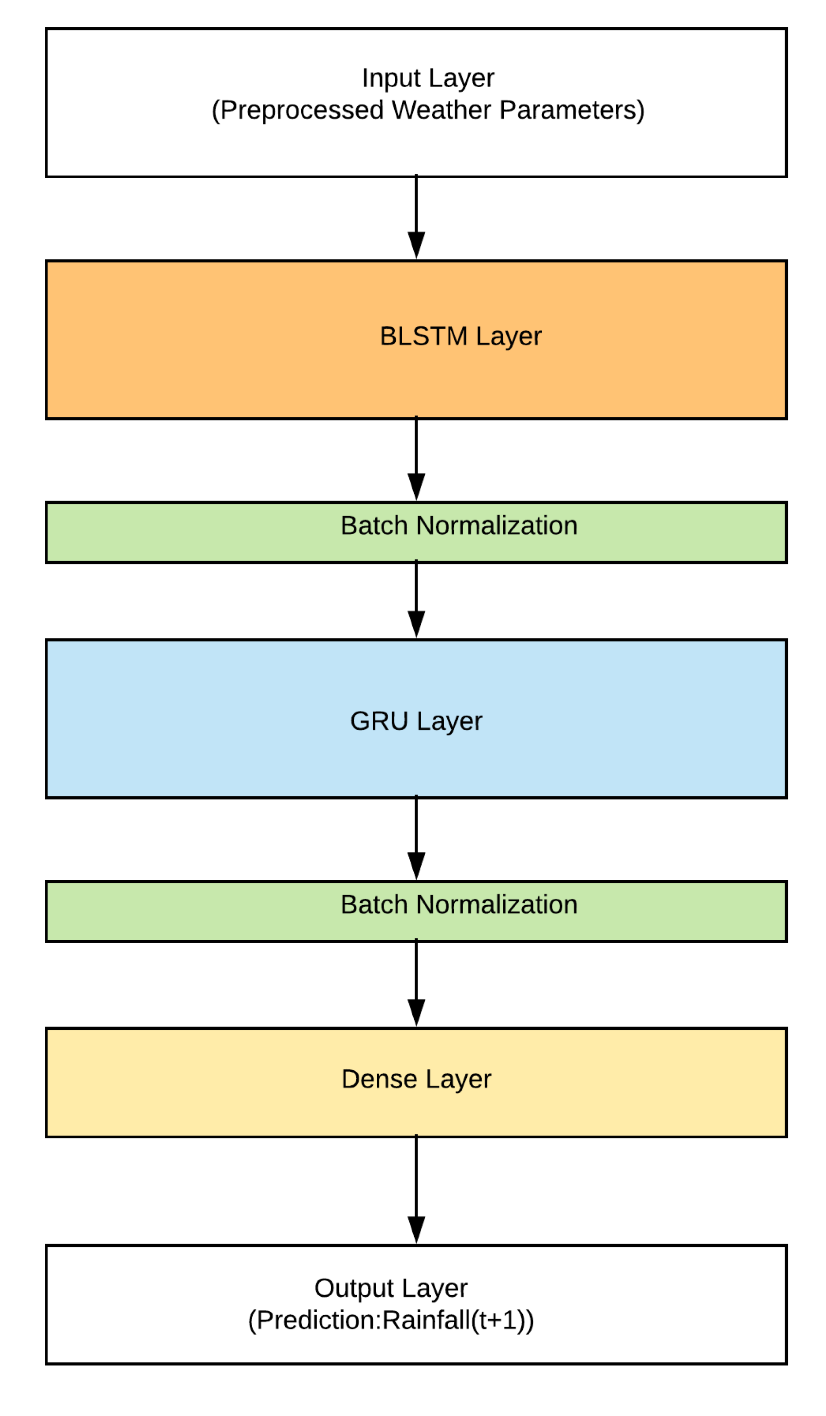
Figure 2.
Map of Bhutan showing major river basins and the annual precipitation (mm). The study area is indicated in the legend.
Figure 2.
Map of Bhutan showing major river basins and the annual precipitation (mm). The study area is indicated in the legend.
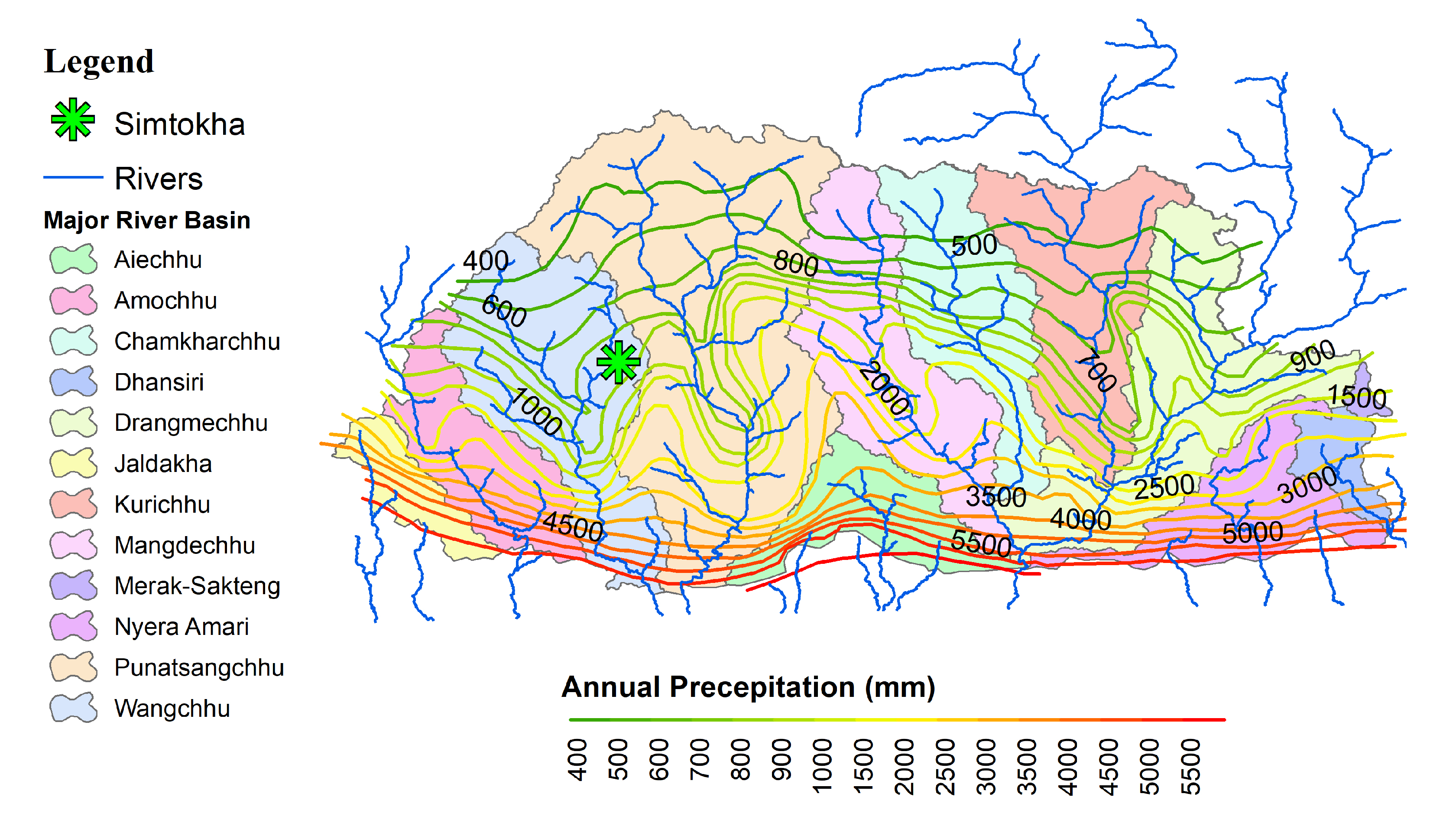
Figure 3.
The subplot of weather parameters used in the study from 1998 to 2018.

Figure 4.
Data preprocessing. The data are preprocessed in 6 stages with the arrowheads showing the flow of data.
Figure 4.
Data preprocessing. The data are preprocessed in 6 stages with the arrowheads showing the flow of data.
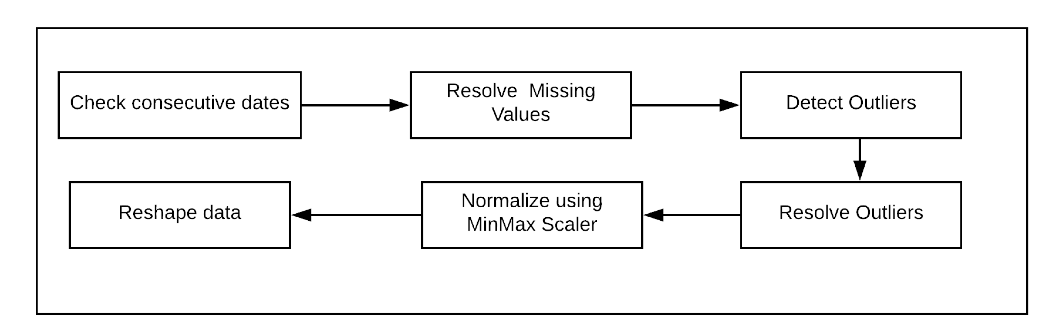
Figure 5.
Many (12) to One LSTM utilized in the experiment. Each sample of data contains 12 time-steps of previous data. We used 12 months of previous data to predict the rainfall of the next month (n + 1).
Figure 5.
Many (12) to One LSTM utilized in the experiment. Each sample of data contains 12 time-steps of previous data. We used 12 months of previous data to predict the rainfall of the next month (n + 1).
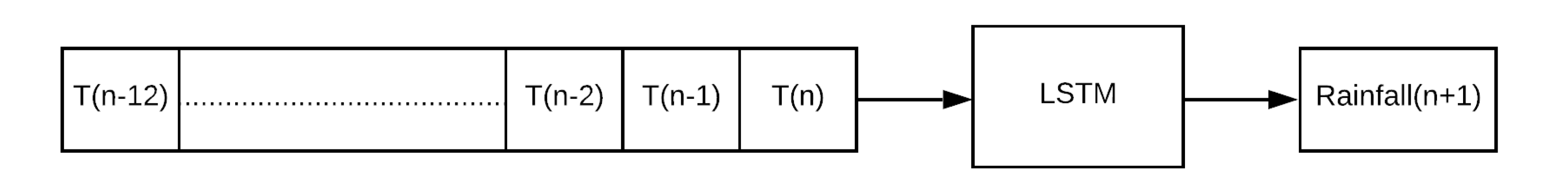
Figure 6.
RMSE and MSE values of 6 existing models including linear regression and the proposed model. It is clear from the figure that our model outperformed the existing models for the same task.
Figure 6.
RMSE and MSE values of 6 existing models including linear regression and the proposed model. It is clear from the figure that our model outperformed the existing models for the same task.
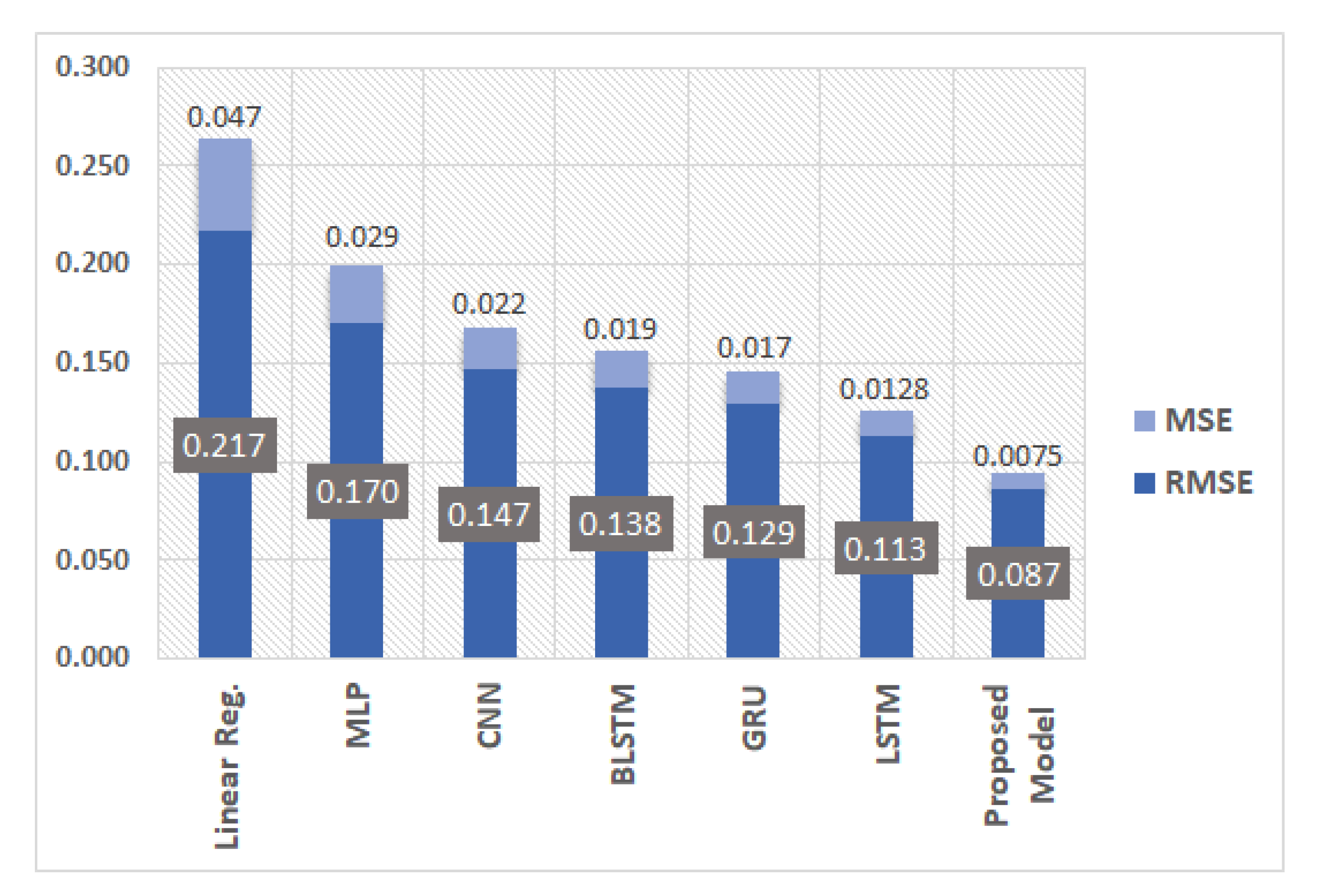
Figure 7.
The plots of actual monthly rainfall values over Simtokha collected from NCHM and predicted rainfall values for the years 2016 and 2017, where the x-axis and y-axis represent months and monthly rainfall values (scaled) respectively. The blue line shows the actual values and the orange line shows the predicted values. Subfigure ‘a’ shows that CNN is not able to predict the peak monthly rainfall values correctly. Results of recurrent neural networks shown by subfigure ‘b’, ‘c’ and ‘d’ are better than that of MLP (subfigure ‘e’). Subfigure ‘f’ shows that the proposed model is able to generalize better and gives the best output.
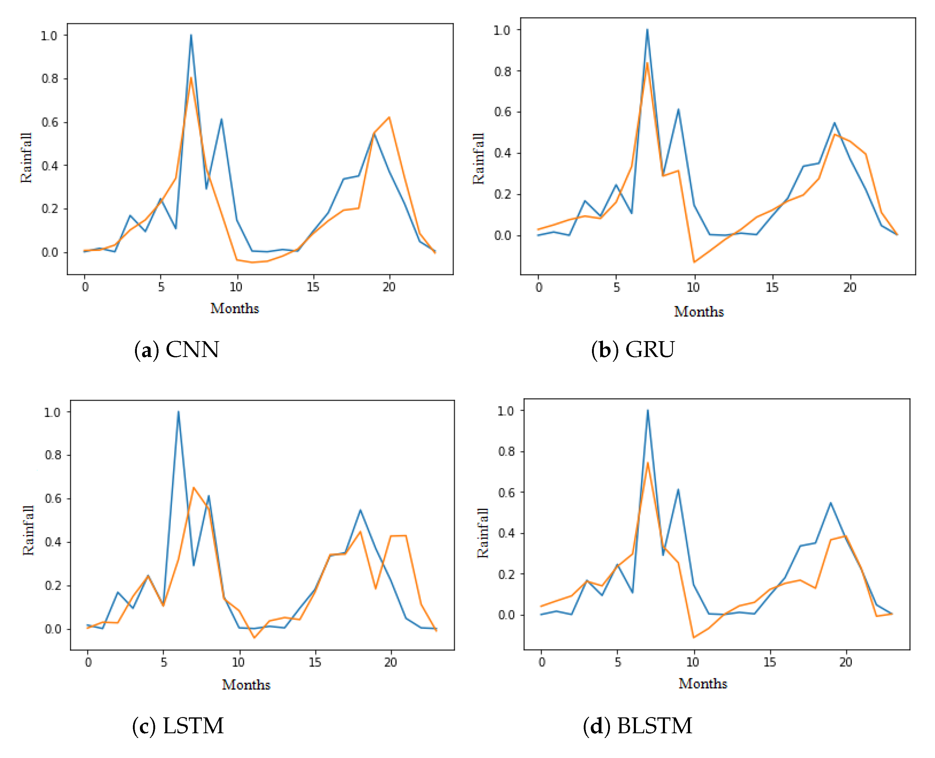

Figure 8.
values of 5 deep learning models and the proposed model.
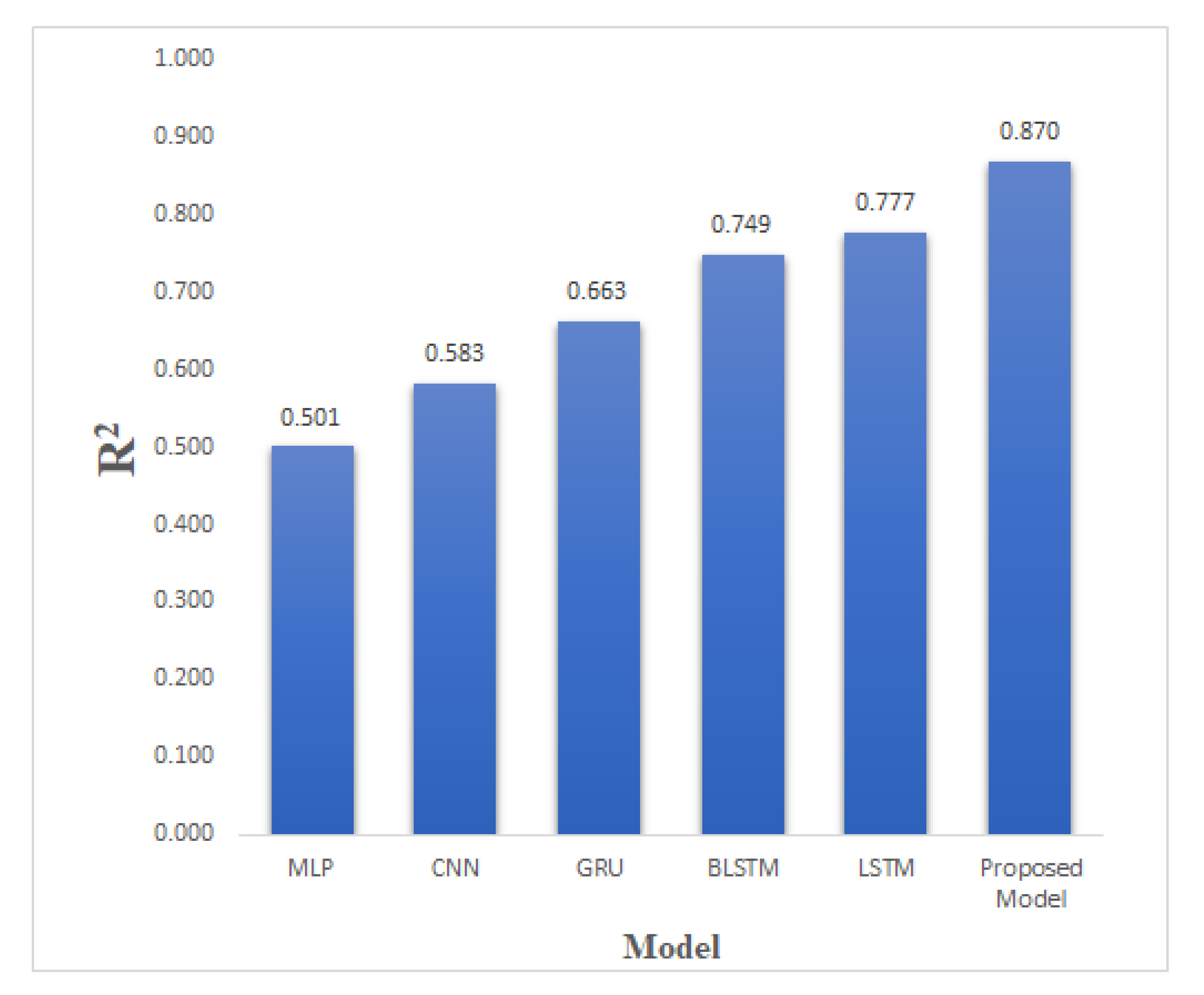
Figure 9.
Pearson Correlation Coefficient values of 5 existing deep learning models and our proposed model. The score of the proposed model was the highest among the models.
Figure 9.
Pearson Correlation Coefficient values of 5 existing deep learning models and our proposed model. The score of the proposed model was the highest among the models.

Table 1.
Related work using Multi-Layer Perceptron.
| Author & Year | Region (Global or Local) | Daily- Monthly- Yearly | Types of NN | Rainfall Predicting Variables | Accuracy Measure |
|---|---|---|---|---|---|
| Luk et al. [12] | Western Sydney | 15 min rainfall prediction | MLFN, PRNN, TDNN | NA | NMSE |
| Huang et al. [11] | Bangkok | 4 years of hourly data from 1997–2003 | MLP and FFNN | NA | Efficiency index (EI) |
| Abhishek et al. [4] | Karnataka, India | 8 months of data from 1960 to 2010 | BPFNN, BPA, LRN and CBP | Average humidity and average wind speed | MSE |
| Nayak et al. [10] | Survey Paper | NA | ANN | NA | NA |
| Darjee et al. [5] | Survey Paper | Monthly, Yearly | ANN, (FFNN, RNN, TDNN) | Maximum and minimum temperatures | NA |
| Hardwinarto et al. [18] | East Kalimantan- Indonesia | Data used from 1986–2008 | BPNN | NA | MSE |
| Khajure et al. [15] | NA | Daily records for 5 years | NN and a fuzzy inference system | Temperature, humidity, dew point, visibility, pressure and windspeed. | MSE |
| Kumar and Tyagi [19] | Nilgiri district Tamil Nadu, India | Monthly rain- fall prediction (Data from 1972–2002) | BPNN, RBFNN | NA | MSE |
| Wahyuni et al. [16] | Tengger East Java | Data used from 2005 to 2014 | BPNN | Changes caused by climate change | RMSE |
| Kashiwao et al. [13] | Japan | Rainfall data from the in- ternet as \“big data” was used. | ANN MLP and RBFN | Atm. pressure, precipitation, humidity, temp., vapor pressure, wind, velocity. | Validation using JMA. |
| Mishra et al. [17] | North India | North India for the period 1871–2012. | FFNN | Rainfall records of previous 2 months and current month | Regression analysis, MRE and MSE |
Table 2.
The parameters used in our study and their corresponding units.
| Rainfall Parameters | Units |
|---|---|
| Maximum Temperature () | C |
| Minimum Temperature () | C |
| Rainfall | Millimeters (mm) |
| Relative Humidity | Percentage (%) |
| Sunshine | Hours (h) |
| Wind Speed | Meters per second (m/s) |
Table 3.
Evaluation metrics for monthly rainfall prediction.
| Name | Formula |
|---|---|
| MSE | |
| RMSE | |
| Correlation |
© 2020 by the authors. Licensee MDPI, Basel, Switzerland. This article is an open access article distributed under the terms and conditions of the Creative Commons Attribution (CC BY) license (http://creativecommons.org/licenses/by/4.0/).
Share and Cite
MDPI and ACS Style
Chhetri, M.; Kumar, S.; Pratim Roy, P.; Kim, B.-G. Deep BLSTM-GRU Model for Monthly Rainfall Prediction: A Case Study of Simtokha, Bhutan. Remote Sens. 2020, 12, 3174. https://doi.org/10.3390/rs12193174
AMA Style
Chhetri M, Kumar S, Pratim Roy P, Kim B-G. Deep BLSTM-GRU Model for Monthly Rainfall Prediction: A Case Study of Simtokha, Bhutan. Remote Sensing. 2020; 12(19):3174. https://doi.org/10.3390/rs12193174
Chicago/Turabian StyleChhetri, Manoj, Sudhanshu Kumar, Partha Pratim Roy, and Byung-Gyu Kim. 2020. "Deep BLSTM-GRU Model for Monthly Rainfall Prediction: A Case Study of Simtokha, Bhutan" Remote Sensing 12, no. 19: 3174. https://doi.org/10.3390/rs12193174
Note that from the first issue of 2016, this journal uses article numbers instead of page numbers. See further details here.