Abstract
Accurate prediction of mineral grades is a fundamental step in mineral exploration and resource estimation, which plays a significant role in the economic evaluation of mining projects. Currently available methods are based either on geometrical approaches or geostatistical techniques that often considers the grade as a regionalised variable. In this paper, we propose a grade estimation technique that combines multilayer feed-forward neural network (NN) and k-nearest neighbour (kNN) models to estimate the grade distribution within a mineral deposit. The models were created by using the available geological information (lithology and alteration) as well as sample locations (easting, northing, and altitude) obtained from the drill hole data. The proposed approach explicitly maintains pattern recognition over the geological features and the chemical composition (mineral grade) of the data. Prior to the estimation of grades, rock types and alterations were predicted at unsampled locations using the kNN algorithm. The presented case study demonstrates that the proposed approach can predict the grades on a test dataset with a mean absolute error (MAE) of and , whereas the traditional model, which only uses the coordinates of sample points as an input, yielded an MAE value of and . The proposed approach is promising and could be an alternative way to estimates grades in a similar modelling tasks.
1. Introduction
One of the critical tasks in mining value chain is to accurately estimate the grades of interest within a mineral deposit. The grades can be in the form of observation or estimation and are used in several stages of mining that ranges from exploration to exploitation. Resource estimation, being one of the initial stages of a mining activity, is an essential step in feasibility studies as well as mine planning [1,2,3,4]. Although the state-of-the-art methodologies used in resource estimation are reasonably advanced in the mining industry, generic application of such methodologies might not be applicable for every complex geological environment [5,6,7,8,9]. Various researchers, therefore, have proposed substantial grade prediction models using diverse techniques such as inverse distance weighing (IDW), kriging and its various versions (simple kriging, ordinary kriging, lognormal kriging, indicator kriging, co-kriging, etc.), and stochastic simulations (sequential Gaussian simulation and sequential indicator simulation) [10,11,12,13,14,15,16]; however, the above-mentioned methods require an assumption in relation to the spatial correlation between samples to be estimated at non-sampled locations [17,18]. In some cases, due to the complex relationships between the grade distribution and spatial pattern variability, geostatistical methods may not give the best estimation results [19]. Consequently, these limitations and complexities inspired researchers to investigate alternative approaches that can be utilised to overcome such obstacles. Over the past few decades, several researchers focused on various computational learning techniques that can predict grades more accurately without having to rely on an underlying assumption [20]. In recent years, machine learning methods, including support vector machine (SVM), random forest (RF), artificial neural network (ANN), and their variations such as support vector regression (SVR) and adaptive neuro-fuzzy inference system (ANFIS), have been used rather extensively to make reliable grade estimations [21,22,23,24,25,26,27,28,29,30,31,32,33,34,35,36,37,38,39,40,41,42,43]. Wu and Zhou, and Yama and Lineberry [44,45] are one of the earliest researchers that used ANN techniques for the grade estimation with an initial success. Kapageridis [46] has utilised a modular neural network system on a randomly sampled iron ore deposit. The comparison made with their proposed approach and kriging demonstrated that the ANN techniques can deliver similar estimate results and requires far less knowledge to be effectively utilised in the estimation. Koike et al. [47] trained an artificial neural network to recognise the relation between the major metal content, location, and lithology of a sample point in the Hokuroku district in Japan. The network model was able to produce a model including many high-content zones based on sample data. Matias et al. [48] compared kriging with regularisation networks (RN), multilayer perceptron (MLP), and radial basis function (RBF) networks for the estimation of the quality of a slate mine. The MLP network showed sufficient results in terms of test error and training speed. Samanta [49] highlights the performance of a radial basis function (RBF) network for ore grade estimation in an offshore placer gold deposit. It was demonstrated that the RBF model produced estimates with the whereas for the traditional kriging prediction method. Jafrasteh et al. [50] investigated the grade prediction performance of machine learning techniques, such as ANN, random forest (RF) and Gaussian process (GP) in the porphyry copper deposit in South-eastern Iran. Their results revealed that GP performed with the best overall accuracy, followed by widely used traditional estimation technique, indicator kriging; however, developing a multilayered ANN model for grade estimation requires the selection of network complexity, which has a direct impact on prediction performance. Network complexity broadly depends on (a) neuron complexity, (b) number of neurons in each layer, (c) number of layers, and (d) number and type of interconnecting weights [51]. Consequently, a number of studies have attempted to solve these problems by combining ANN with other computational techniques. Mahmoudabadi et al. [52] proposed a hybrid method that utilizes the combination of the Levenberg–Marquardt (LM) method and genetic algorithm (GA) to identify the ANNs optimal initial weights. Chatterjee et al. [53] suggest an ensemble of neural networks utilising a genetic algorithm (GA) and k-means clustering modelling of a lead–zinc deposit. Several network models were trained, and the best models were selected for improving the accuracy of the ensemble model. Results revealed that the GA-based model outperformed the other models considered. Although the literature review highlights the potential benefits of machine learning methods in accurate grade estimation on variety of case studies, they also mention various drawbacks as well. For instance, there is no certain rule to determine the network hyper-parameters. Proper structure can only be achieved by trial and error, which is a computationally intensive procedure. Another critical issue is that once an ANN provides a solution, it does not give any explanation regarding the possible relationship with input; therefore, there is still room for further investigation of data-driven learning models in order to obtain accurate grade estimation.
The aim of this paper is to present a new grade modelling approach that combines k-nearest neighbour (kNN) and ANN models to perform grade estimations of a mineral deposit. The proposed approach utilises geological information (lithology and alteration) and spatial information (easting, northing, and altitude) for the model creation. The model creation is comprised of two steps. First, the kNN model is trained to predict rock types and alteration levels. This model allows us to estimate the geological information at non-sampled locations as a first step. Second, the ANN model is trained to predict grades using the geological and spatial information. The ANN model utilises the geological information predictions made by the kNN model as well as the geographic information as input variables. When the model is trained with sufficient data, the network is able to learn the relationship between input variables (rock type, alteration level, and geographic position) and the output variable, which is grade.
This article is organised as follows: Section 2 presents brief information on the dataset used to demonstrate the methodology and data pre-processing. Section 3 presents the model development and implementations on a real case study. Section 4 presents the analyses of the results and discusses the findings. Finally, the conclusions of the paper are presented in Section 5.
2. Data Attributes and Preparation
In this study, data were collected from a gold deposit during the second phase of a resource drilling program. Most of the study area is underlain by mafic, intermediate, more rarely felsic volcanic rocks and associated volcano-sedimentary formations that are cross-cut by post tectonic granitoids. Due to confidentiality agreement, Authors do not have a permission to refer the name of deposit, location, or any other mineralization characteristics that might expose the deposit and/or the mining company. The study area extends over 2 × 3 km2 and the data contains gold grade values (ppm) from 123 drill holes. The average distance between drill holes is approximately 25 m (Figure 1). The average length of the boreholes is about 100 m. Samples from the boreholes were collected at intervals of 1 m. The ore is extracted from ten different lithologies. For the present study, raw borehole data were composited based on the lithology, which produced 4721 composited intervals altogether.
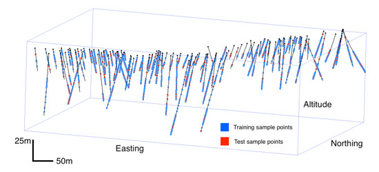
Figure 1.
Location of train and test sample points.
Raw borehole data that comes from a drill hole is unusable for neural network training due to (a) intense spatial grade variability, (b) unequal sample length, (c) noise due to outlier data points that differs significantly from other observations, and (d) varying range of numerical values existing in the dataset for different variables. Several preparation steps had to be performed to be able to use the raw data in the ANN model. These steps are as follows:
- Step 1. Creating a composite data: Raw data comes from 123 drill holes were composited in 1 m length, which is equal to the average sample length in one run. Table 1 presents the descriptive statistics of the composite dataset.
 Table 1. Basic statistics of the composited dataset.
 - Step 2. Data pre-processing: Each sample is described by five attributes including coordinates (easting, northing, and altitude), rock type, and alteration level. The original raw data contains 25 different rock types and 5 different alteration types. To generalise the geological distribution, we combined similar lithologies to reduce the original rock type to 10 and used only level of argillic alteration (a0, a1, ..., a4) that shows the high correlation with gold grade.
- Step 3. Transformation of the categorical data into numerical values: Neural Network (NN) algorithm performs numerical calculations; therefore, it can only operate with numerical numbers; however, lithology code and alteration level that is present in the dataset has categorical values denoted by characters (GG, AC, a1, a4, etc.). To feed the ANN with numerical information, original categorical values were transformed into Boolean variables through hot-encoding, as can be seen in Table 2. This resulted in representing each of the rock types and alteration level in a series of 0 or 1 values which indicate the absence or presence of a specified condition.
Table 2. Some of sample points from the training dataset.
- Step 4. Data normalisation: In order to handle various data types and ranges existing in the dataset (i.e., geographical coordinates and grades), the values in each feature were normalised based on the mean and standard deviation. This was performed to scale different values of features into a common scale [54]. The value of a data point in each feature was recalculated by subtracting the population mean of a given feature from an individual point and then dividing the difference by the standard deviation of the population [55]. Each instance, of the data is transformed into as follows:where and denote the mean and standard deviation of ith feature respectively [56].
- Step 5. Splitting dataset into training/test sets: To evaluate the model performance, the dataset was randomly divided into training (80% of the data) and testing sets (20% of the data). The model was only trained using the training data. Its performance was validated using testing dataset. It is important to point out that these two data sets have similar statistical attributes.
3. Model Development and Implementations
To construct the NN model in this study, spatial positions (easting, northing, and altitude), rock types, and alteration levels were used as inputs to predict the Au grade [57]. To make a prediction at each sample point, it is essential to provide the rock type and alteration information. In fact, this information is only available at the borehole locations. Hence, to use the NN model, rock type and alteration information need be provided for each non-sampled location at which the grade values are to be estimated. This was achieved by using the trained kNN model to make predictions at non-sampled locations.
3.1. Lithology and Alteration Prediction
Since its introduction by Thomas Cover [58], kNN has been widely used to solve nearly every regression and classification problem. For a given test query, kNN algorithm finds k-closest points in feature space and performs a prediction based on the values at k-closest neighbours. It repeats this for all the test data; therefore, it is often classified as “instance-based learning”, or “lazy learning”. Detailed descriptions of the kNN algorithm can be found in a number of textbooks [59,60,61,62]. In this study, a kNN model was developed to predict rock types and alterations at unknown locations. Python 3.6.9 [63] programming language and Scikit-learn [64] machine learning library were used to create the kNN model. The model requires the specification of k-number of neighbours to be used as a hyper-parameter, which is highly specific for a given dataset; therefore, choosing of the optimal k-value is needed prior to the model creation. A small k-value could add noise that would have significant influence on the final model. In contrast, a large k-value would create over-fitting. In this research, grid search with k-fold (K-5) cross-validation was used for determining optimal hyper-parameters for kNN algorithm. Given an acceptable search range, a grid search was applied on all possible values and “best” parameter setting minimising the losses was picked. Once the k parameter was specified, the kNN model was created and the performance of it was evaluated using the test dataset. It should be noted that the training dataset used to create the kNN model was also used for the development of the ANN model. Chosen hyper-parameters of the kNN model can be seen in Table 3.
Table 3.
Hyper-parameters for the k-nearest neighbours (kNN) model.
3.2. Neural Network Model for Grade Estimation
Since the chemical composition of mineral deposit is highly correlated with alteration and lithology, building a three-dimensional geologic model is a crucial step for predicting an accurate grade distribution. After trying a variety of NN configuration, best results with minimum error rate were obtained by an NN architecture comprising one input layer which consists of 18 neurons, 2 hidden layers each of which has 64 neurons, and 1 neuron output layer (Figure 2). The model was built using the Python 3.6.9 programming language and Keras 2.2.5 [65] deep learning library.
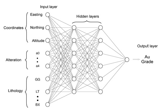
Figure 2.
Proposed NN model architecture.
In order to compare the model performance against the traditional NN modelling approach in literature, we first created a separate NN model for comparison purposes. This model only uses the sample locations (coordinates) as input variables for the network to predict the Au grade. We then created the proposed model, which not only utilises the sample locations to model the grade distribution, but also the rock type and alteration levels that were predicted by the kNN algorithm. This model corresponds to the NN model. To compare the network prediction performance, NN was fed by location, rock type, and alteration, which already known. This model corresponds to real NN model. Once the three models were created, they were run on the independent test set (unseen and unused by model) to evaluate the model accuracies.
The back-propagation algorithm was used for training the neural network. It is a widely used iterative gradient algorithm designed to minimise the error between the true and predicted model outputs [66,67]. As an optimisation algorithm, RMSProp has been applied to update the weight tensors () during training. RMSProp utilises an adaptive learning rate rather than a predefined one. It uses a moving average squared gradient to normalise the gradients [68]. A user defined loss function is used to evaluate the predictions against the targets and produces an error value, which is used during training to update the weights (Figure 3).
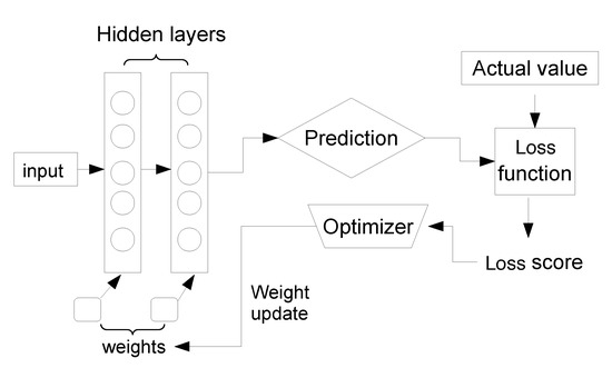
Figure 3.
Interrelationship between loss function and optimiser.
To determine the hyper-parameters of the NN model, k-fold cross validation [69] was used. We set the k-value to 5; therefore, our training set comprised 5 different equally sized partitions, each of which is comprised of 80% training dataset as for training the model and 20% of the training dataset as for model validation. For each partition, we train a network model on the remaining ‘K-1’ partitions and evaluate its accuracy on partition ‘K’ (Figure 4). Average of the losses obtained from the folds is used for the training loss. Training hyper-parameters such as number of epochs, optimiser, and learning rate were determined based on trial and error method.
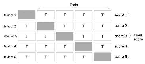
Figure 4.
5-fold cross-validation to optimise the performances of the resulting models.
In this paper, three performance metrics, mean absolute error (MAE), mean square error (MSE), and coefficient of determination (), were used to evaluate the prediction performance. Figure 5 shows MAE improvement for each epoch on training data set. To avoid network over-fitting, which is a typical issue for NN applications, 400 epoch were used for model prediction.
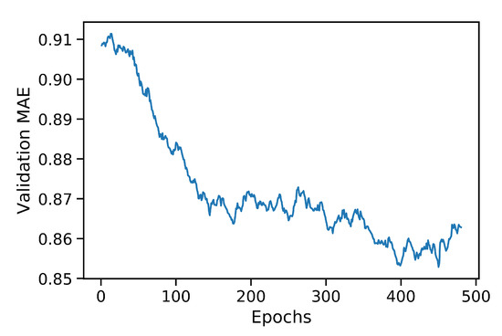
Figure 5.
Mean absolute error (MAE) for every generation during the NN training process.
4. Results and Discussion
To assess the model prediction performance, the dataset was randomly divided 30 subsets as described earlier in Section 2. Table 4 and Figure 6 summarizes the Au grade prediction results for every simulation using each subset of data. For each simulation, the test subsets were used for evaluating the performance of the kNN and NN models. Results of Simulation 23 shown in Table 5, Table 6, Table 7, Table 8, Table 9 and Table 10, the prediction performances of the created kNN model on rock type estimations is similar to that of alteration (80% and 74%, respectively). Although the kNN model appears to have a reasonable estimation accuracy for high rock type estimations, the model did not make any QVS lithology predictions. This is considered to be stemming from the insufficient QVS samples in the training set. Actual QVS lithologies were confused with QV lithologies.
Table 4.
NN model simulation summary.
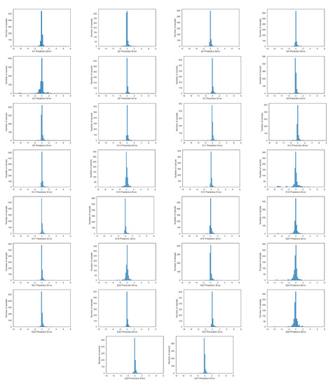
Figure 6.
Histogram of prediction errors for 30 simulations.
Table 5.
kNN model lithology predictions.
Table 6.
kNN model lithology prediction score.
Table 7.
kNN model alteration predictions.
Table 8.
kNN model alteration prediction score.
Table 9.
Performance comparison.
Table 10.
Simulation 23, Comparison of NN models predictions.
For each test point, sample locations (easting, northing, and altitude) and lithological features were used as input values to get the mineral grade estimates. The suggested NN model in literature yielded a for MAE and for in Simulation 23. When the model only used the sample locations as input variables (traditional ANN model), MAE of and of were obtained (Table 9). This demonstrates the fact that the grades can be better estimated if lithological features such as rock type and alteration levels were also used (Figure 7, Figure 8 and Figure 9).
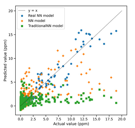
Figure 7.
Simulation 23 actual versus predicted values on the testing data for each model.
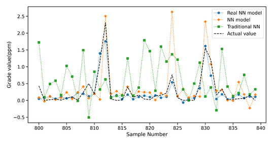
Figure 8.
Simulation 23, comparison of NN models predictions.
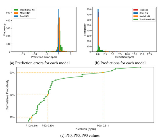
Figure 9.
Simulation 23, histogram of prediction performances and p-values.
As it can be seen in Figure 10, Model NN and Real NN models provide the closest real distribution grades as compared to traditional NN.
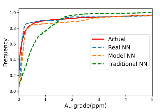
Figure 10.
Simulation 23, cumulative distribution of actual and NN models.
The results have shown that the suggested model has underestimated any grades between 15 ppm and 20 ppm range. Close examination of sample points shows that in the condition where mineralization is controlled by the structure and a test point located near a fault, the network could not ignore the effect of discontinuity of lithology. The proposed model stands on lithological control of mineralization, and it is relatively immune to systems that is structurally controlled. Another notable outcome is that the NN model failed to predict some of the sample points that have a high number of samples in the training set. It could be partly due to a neural network can be successfully utilised to execute probabilistic functions [70]; however, no matter how much network is trained in order to improve the prediction, independent stochastic events cannot be predicted by any neural network models.
5. Conclusions
Accurate grade estimation is a significant part of a mining project, as it highly influences the decisions made in both exploration and exploitation stages of mining process. In this paper, we proposed a grade estimation methodology that utilises kNN and multilayer feed forward neural network that incorporates sample locations, lithological features, and alteration levels. It has been shown in the paper that the a kNN–NN hybrid model can be successfully utilised in a grade estimation task. The proposed model does not require complicated mathematical knowledge or deep assumptions. It is a data-driven method to that utilises the relationship between input and output values. Since the model incorporated geological features, alteration levels, and sample coordinates in the learning process, it can be tailored to fit any other grade modelling tasks. Although the model successfully figured out the relationship between the input and output variables, it ignored the structural influence of mineralization, which is expected as it is generally difficult to recognise. The proposed approach primarily provides the following advantages:
- The grade estimation can be more accurately modelled by having an intermediate modelling step that predicts rock types and alteration features as an input for the subsequent NN model.
- The suggested model does not require any assumptions on the input variables as in geostatistics.
- The method can be easily modified and applied into other mining resources as compared to classical resource estimation techniques.
While the proposed method has the significant advantages, the following drawbacks requires further attention in the application of the proposed method in different cases.
- Inadequate data and depth of network can easily cause over-fitting issues in complex NN structures. The network is highly sensitive to following hyper-parameters: number of hidden layers, activation function type, number of epoch, and learning rate.
- The suggested model is based on lithological control of mineralization and is highly sensitive to the existence of geological discontinuities.
It would be worth it to compare the proposed method with the traditional geostatistical methods on a case study. Furthermore, log of the grade values can be use instead of direct grades itself in the ANN model generations. Comparison of the predicted grades generated by direct value of grades itself vs. log value of the grades can be investigated as future research.
Author Contributions
U.E.K. and E.T. contributed equally to this work. All authors have read and agreed to the published version of the manuscript.
Funding
This research received no external funding.
Conflicts of Interest
The authors declare no conflict of interest.
References
- Weeks, R.M. Ore reserve estimation and grade control at the Quemont mine. In Proceedings of the Ore Reserve Estimation and Grade Control: A Canadian Centennial Conference Sponsored by the Geology and Metal Mining Divisions of the CIM, Ville d’Esterel, QC, Canada, 25–27 September 1967; Canadian Institute of Mining and Metallurgy: Westmount, QC, Canada, 1968; Volume 9, p. 123. [Google Scholar]
- Sinclair, A.J.; Blackwell, G.H. Applied Mineral Inventory Estimation; Cambridge University Press: Cambridge, UK, 2002. [Google Scholar]
- Akbari, A.D.; Osanloo, M.; Shirazi, M.A. Reserve estimation of an open pit mine under price uncertainty by real option approach. Min. Sci. Technol. 2009, 19, 709–717. [Google Scholar] [CrossRef]
- Rendu, J.M. An Introduction to Cut-Off Grade Estimation; Society for Mining, Metallurgy, and Exploration: Englewood, CO, USA, 2014. [Google Scholar]
- Joseph, V.R. Limit kriging. Technometrics 2006, 48, 458–466. [Google Scholar] [CrossRef]
- Armstrong, M. Problems with universal kriging. J. Int. Assoc. Math. Geol. 1984, 16, 101–108. [Google Scholar] [CrossRef]
- Cressie, N. The origins of kriging. Math. Geol. 1990, 22, 239–252. [Google Scholar] [CrossRef]
- Isaaks, E.H.; Srivastava, M.R. Applied Geostatistics; Number 551.72 ISA; Oxford University Press: Oxford, UK, 1989. [Google Scholar]
- Matheron, G. Principles of geostatistics. Econ. Geol. 1963, 58, 1246–1266. [Google Scholar] [CrossRef]
- Journel, A.G.; Huijbregts, C.J. Mining Geostatistics; Academic Press: London, UK, 1978; Volume 600. [Google Scholar]
- Rendu, J. Kriging, logarithmic Kriging, and conditional expectation: Comparison of theory with actual results. In Proceedings of the 16th APCOM Symposium, Tucson, Arizona, 17–19 October 1979; pp. 199–212. [Google Scholar]
- Cressie, N. Spatial prediction and ordinary kriging. Math. Geol. 1988, 20, 405–421. [Google Scholar] [CrossRef]
- Goovaerts, P. Geostatistics for Natural Resources Evaluation; Oxford University Press: Oxford, UK, 1997. [Google Scholar]
- Chiles, J.P.; Delfiner, P. Modeling spatial uncertainty. In Geostatistics, Wiley Series in Probability and Statistics; John Wiley & Sons: New York, NY, USA, 1999. [Google Scholar]
- David, M. Geostatistical Ore Reserve Estimation; Elsevier: Amsterdam, The Netherlands, 2012. [Google Scholar]
- Paithankar, A.; Chatterjee, S. Grade and tonnage uncertainty analysis of an african copper deposit using multiple-point geostatistics and sequential Gaussian simulation. Nat. Resour. Res. 2018, 27, 419–436. [Google Scholar] [CrossRef]
- Badel, M.; Angorani, S.; Panahi, M.S. The application of median indicator kriging and neural network in modeling mixed population in an iron ore deposit. Comput. Geosci. 2011, 37, 530–540. [Google Scholar] [CrossRef]
- Tahmasebi, P.; Hezarkhani, A. Application of a modular feedforward neural network for grade estimation. Nat. Resour. Res. 2011, 20, 25–32. [Google Scholar] [CrossRef]
- Pan, G.; Harris, D.P.; Heiner, T. Fundamental issues in quantitative estimation of mineral resources. Nonrenew. Resour. 1992, 1, 281–292. [Google Scholar] [CrossRef]
- Jang, H.; Topal, E. A review of soft computing technology applications in several mining problems. Appl. Soft Comput. 2014, 22, 638–651. [Google Scholar] [CrossRef]
- Singer, D.A.; Kouda, R. Application of a feedforward neural network in the search for Kuroko deposits in the Hokuroku district, Japan. Math. Geol. 1996, 28, 1017–1023. [Google Scholar] [CrossRef]
- Denby, B.; Burnett, C. A neural network based tool for grade estimation. In Proceedings of the 24th International Symposium on the Application of Computer and Operation Research in the Mineral Industries (APCOM), Montreal, QC, Canada, 31 October–3 November 1993. [Google Scholar]
- Clarici, E.; Owen, D.; Durucan, S.; Ravencroft, P. Recoverable reserve estimation using a neural network. In Proceedings of the 24th International Symposium on the Application of Computer and Operation Research in the Mineral Industries (APCOM), Montreal, QC, Canada, 31 October–3 November 1993; pp. 145–152. [Google Scholar]
- Ke, J. Neural Network Modeling of Placer Ore Grade Spatial Variability. Ph.D. Thesis, University of Alaska Fairbanks, Fairbanks, AK, USA, 2002. [Google Scholar]
- Koike, K.; Matsuda, S. Characterizing content distributions of impurities in a limestone mine using a feedforward neural network. Nat. Resour. Res. 2003, 12, 209–222. [Google Scholar] [CrossRef]
- Koike, K.; Matsuda, S.; Gu, B. Evaluation of interpolation accuracy of neural kriging with application to temperature-distribution analysis. Math. Geol. 2001, 33, 421–448. [Google Scholar] [CrossRef]
- Porwal, A.; Carranza, E.; Hale, M. A hybrid neuro-fuzzy model for mineral potential mapping. Math. Geol. 2004, 36, 803–826. [Google Scholar] [CrossRef]
- Samanta, B.; Bandopadhyay, S.; Ganguli, R. Data segmentation and genetic algorithms for sparse data division in Nome placer gold grade estimation using neural network and geostatistics. Explor. Min. Geol. 2002, 11, 69–76. [Google Scholar] [CrossRef]
- Samanta, B.; Ganguli, R.; Bandopadhyay, S. Comparing the predictive performance of neural networks with ordinary kriging in a bauxite deposit. Min. Technol. 2005, 114, 129–139. [Google Scholar] [CrossRef]
- Singer, D.A. Typing mineral deposits using their associated rocks, grades and tonnages using a probabilistic neural network. Math. Geol. 2006, 38, 465–474. [Google Scholar] [CrossRef]
- Chatterjee, S.; Bhattacherjee, A.; Samanta, B.; Pal, S.K. Ore grade estimation of a limestone deposit in India using an artificial neural network. Appl. GIS 2006, 2, 1–20. [Google Scholar] [CrossRef]
- Misra, D.; Samanta, B.; Dutta, S.; Bandopadhyay, S. Evaluation of artificial neural networks and kriging for the prediction of arsenic in Alaskan bedrock-derived stream sediments using gold concentration data. Int. J. Min. Reclam. Environ. 2007, 21, 282–294. [Google Scholar] [CrossRef]
- Dutta, S.; Bandopadhyay, S.; Ganguli, R.; Misra, D. Machine learning algorithms and their application to ore reserve estimation of sparse and imprecise data. J. Intell. Learn. Syst. Appl. 2010, 2, 86. [Google Scholar] [CrossRef]
- Pham, T.D. Grade estimation using fuzzy-set algorithms. Math. Geol. 1997, 29, 291–305. [Google Scholar] [CrossRef]
- Tutmez, B. An uncertainty oriented fuzzy methodology for grade estimation. Comput. Geosci. 2007, 33, 280–288. [Google Scholar] [CrossRef]
- Tahmasebi, P.; Hezarkhani, A. Application of adaptive neuro-fuzzy inference system for grade estimation; case study, Sarcheshmeh porphyry copper deposit, Kerman, Iran. Aust. J. Basic Appl. Sci. 2010, 4, 408–420. [Google Scholar]
- Tahmasebi, P.; Hezarkhani, A. A hybrid neural networks-fuzzy logic-genetic algorithm for grade estimation. Comput. Geosci. 2012, 42, 18–27. [Google Scholar] [CrossRef]
- Rodriguez-Galiano, V.; Sanchez-Castillo, M.; Chica-Olmo, M.; Chica-Rivas, M. Machine learning predictive models for mineral prospectivity: An evaluation of neural networks, random forest, regression trees and support vector machines. Ore Geol. Rev. 2015, 71, 804–818. [Google Scholar] [CrossRef]
- Jafrasteh, B.; Fathianpour, N.; Suárez, A. Advanced machine learning methods for copper ore grade estimation. In Proceedings of the Near Surface Geoscience 2016-22nd European Meeting of Environmental and Engineering Geophysics, Helsinki, Finland, 4–6 September 2006; European Association of Geoscientists & Engineers: Houten, The Netherlands, 2016. Number 1. p. cp-495-00087. [Google Scholar] [CrossRef]
- Das Goswami, A.; Mishra, M.; Patra, D. Investigation of general regression neural network architecture for grade estimation of an Indian iron ore deposit. Arab. J. Geosci. 2017, 10, 80. [Google Scholar] [CrossRef]
- Jafrasteh, B.; Fathianpour, N. A hybrid simultaneous perturbation artificial bee colony and back-propagation algorithm for training a local linear radial basis neural network on ore grade estimation. Neurocomputing 2017, 235, 217–227. [Google Scholar] [CrossRef]
- Zhao, X.; Niu, J. Method of Predicting Ore Dilution Based on a Neural Network and Its Application. Sustainability 2020, 12, 1550. [Google Scholar] [CrossRef]
- Maleki, M.; Jélvez, E.; Emery, X.; Morales, N. Stochastic Open-Pit Mine Production Scheduling: A Case Study of an Iron Deposit. Minerals 2020, 10, 585. [Google Scholar] [CrossRef]
- Wu, X.; Zhou, Y. Reserve estimation using neural network techniques. Comput. Geosci. 1993, 19, 567–575. [Google Scholar] [CrossRef]
- Yama, B.; Lineberry, G. Artificial neural network application for a predictive task in mining. Min. Eng. 1999, 51, 59–64. [Google Scholar]
- Kapageridis, I.; Denby, B. Ore grade estimation with modular neural network systems—A case study. In Information Technology in the Mineral Industry; Panagiotou, G.N., Michalakopoulos, T.N., Eds.; AA Balkema Publishers: Rotterdam, The Netherlands, 1998; p. 52. [Google Scholar]
- Koike, K.; Matsuda, S.; Suzuki, T.; Ohmi, M. Neural network-based estimation of principal metal contents in the Hokuroku district, northern Japan, for exploring Kuroko-type deposits. Nat. Resour. Res. 2002, 11, 135–156. [Google Scholar] [CrossRef]
- Matias, J.; Vaamonde, A.; Taboada, J.; González-Manteiga, W. Comparison of kriging and neural networks with application to the exploitation of a slate mine. Math. Geol. 2004, 36, 463–486. [Google Scholar] [CrossRef]
- Samanta, B. Radial basis function network for ore grade estimation. Nat. Resour. Res. 2010, 19, 91–102. [Google Scholar] [CrossRef]
- Jafrasteh, B.; Fathianpour, N.; Suárez, A. Comparison of machine learning methods for copper ore grade estimation. Comput. Geosci. 2018, 22, 1371–1388. [Google Scholar] [CrossRef]
- Chaturvedi, D. Factors affecting the performance of artificial neural network models. In Soft Computing: Techniques and Its Applications in Electrical Engineering; Springer: Berlin/Heidelberg, Germany, 2008; pp. 51–85. [Google Scholar]
- Mahmoudabadi, H.; Izadi, M.; Menhaj, M.B. A hybrid method for grade estimation using genetic algorithm and neural networks. Comput. Geosci. 2009, 13, 91–101. [Google Scholar] [CrossRef]
- Chatterjee, S.; Bandopadhyay, S.; Machuca, D. Ore grade prediction using a genetic algorithm and clustering based ensemble neural network model. Math. Geosci. 2010, 42, 309–326. [Google Scholar] [CrossRef]
- Sola, J.; Sevilla, J. Importance of input data normalization for the application of neural networks to complex industrial problems. IEEE Trans. Nucl. Sci. 1997, 44, 1464–1468. [Google Scholar] [CrossRef]
- Larsen, R.J.; Marx, M.L. An Introduction to Mathematical Statistics and Its Applications; Prentice Hall: London, UK, 2005. [Google Scholar]
- Singh, D.; Singh, B. Investigating the impact of data normalization on classification performance. Appl. Soft Comput. 2019, 105524. [Google Scholar] [CrossRef]
- Kaplan, U.E. Method for Determining Ore Grade Using Artificial Neural Network in a Reserve Estimation. Australia Patent Au2019101145, 30 September 2019. [Google Scholar]
- Cover, T.; Hart, P. Nearest neighbor pattern classification. IEEE Trans. Inf. Theory 1967, 13, 21–27. [Google Scholar] [CrossRef]
- Altman, N.S. An introduction to kernel and nearest-neighbor nonparametric regression. Am. Stat. 1992, 46, 175–185. [Google Scholar]
- Davis, J.C. Introduction to Statistical Pattern Recognition. Comput. Geosci. 1996, 7, 833–834. [Google Scholar] [CrossRef]
- Fukunaga, K. Introduction to Statistical Pattern Recognition; Elsevier: Amsterdam, The Netherlands, 2013. [Google Scholar]
- Peterson, L.E. K-nearest neighbor. Scholarpedia 2009, 4, 1883. [Google Scholar] [CrossRef]
- Van Rossum, G.; Drake, F.L., Jr. Python Tutorial; Centrum voor Wiskunde en Informatica: Amsterdam, The Netherlands, 1995. [Google Scholar]
- Pedregosa, F.; Varoquaux, G.; Gramfort, A.; Michel, V.; Thirion, B.; Grisel, O.; Blondel, M.; Prettenhofer, P.; Weiss, R.; Dubourg, V.; et al. Scikit-learn: Machine Learning in Python. J. Mach. Learn. Res. 2011, 12, 2825–2830. [Google Scholar]
- Keras. Available online: https://keras.io (accessed on 25 February 2019).
- Parker, D.B. Learning Logic. Invention Report S81-64, File 1; Oce of Technology Licensing; Stanford University: Paolo Alto, CA, USA, 1982. [Google Scholar]
- Rumelhart, D.E.; Hinton, G.E.; Williams, R.J. Learning representations by back-propagating errors. Nature 1986, 323, 533–536. [Google Scholar] [CrossRef]
- Hinton, G.; Srivastava, N.; Swersky, K. Neural networks for machine learning lecture 6a overview of mini-batch gradient descent. Cited 2012, 14, 1–31. [Google Scholar]
- Harrell, F.E., Jr. Regression Modeling Strategies: With Applications to Linear Models, Logistic and Ordinal Regression, and Survival Analysis; Springer: Berlin/Heidelberg, Germany, 2015. [Google Scholar]
- Pagel, J.F.; Kirshtein, P. Machine Dreaming and Consciousness; Academic Press: Cambridge, MA, USA, 2017. [Google Scholar]
© 2020 by the authors. Licensee MDPI, Basel, Switzerland. This article is an open access article distributed under the terms and conditions of the Creative Commons Attribution (CC BY) license (http://creativecommons.org/licenses/by/4.0/).