Black Hole Evaporation: A Perspective from Loop Quantum Gravity

Institute for Gravitation and the Cosmos, Penn State University, University Park, PA 16801, USA
Universe 2020, 6(2), 21; https://doi.org/10.3390/universe6020021
Submission received: 9 December 2019
/
Revised: 20 January 2020
/
Accepted: 20 January 2020
/
Published: 24 January 2020
(This article belongs to the Special Issue Probing New Physics with Black Holes)
Abstract
:A personal perspective on the black hole evaporation process is presented using, as guidelines, inputs from: (i) loop quantum gravity, (ii) simplified models where concrete results have been obtained, and, (iii) semi-classical quantum general relativity. On the one hand, the final picture is conservative in that there are concrete results that support each stage of the argument, and there are no large departures from general relativity or semi-classical gravity in tame regions outside macroscopic black holes. On the other hand, it argues against certain views that are commonly held in many quarters, such as persistence of a piece of singularity that constitutes a part of the final boundary of space–time; presence of an event horizon serving as an absolute barrier between the interior and the exterior, and the (often implicit) requirement that purification must be completed by the time the ‘last rays’ representing the extension of this event horizon reach .
1. Introduction
Figure 1a is the standard Penrose diagram of the gravitational collapse of a star to form a non-rotating black hole in classical general relativity (GR). While serves as the past boundary of this space–time, constitutes only a part of the future boundary which also includes the future, space-like singularity. Therefore, while data for a zero rest mass field on suffices to determine the field everywhere in space–time in the forward (in time) evolution, data on is clearly insufficient in the backward evolution; the singularity ‘soaks up part of the information’ in generic solutions to field equations.
Hawking’s celebrated 1975 calculation [1] was carried out on this space–time, ignoring the back reaction. However, he also drew the Penrose diagram he expected to result once the back reaction is appropriately taken into account, shown in Figure 1b. This diagram is routinely used in many discussions of the black hole evaporation process and the associated issue of potential information loss. It depicts the idea that, as the back hole loses energy through radiation to , the ‘strength’ of the singularity—captured by, say, the Kretschmann scalar that goes as in spherically symmetric space–times—diminishes and so the singularity ends, rather than extending all the way to as in Figure 1a. Fluctuations in the vacuum at are excited resulting in the creation of pairs of modes, one escaping to and its partner falling into the singularity. If this were an accurate depiction of the process, then evolution from an early time (or initial) Cauchy surface to a late time surface (or final) would not be unitary because the partner modes disappear into the black hole. Therefore, Hawking was led to introduce a generalization of the standard (unitary) S-matrix to a $-operator that can evolve pure states to mixed [2]. By and large, there is consensus in the relativity community that this conclusion would be inescapable if Figure 1b were to faithfully capture the full evaporation process. However, it is important to note that Hawking’s original space–time diagram [1] was not based on a detailed calculation; rather, it expressed his then expectation on how evaporation would proceed. Interestingly, by 2016 his expectation changed completely. A new Penrose diagram was proposed in [3] (their Figure 2) in which there is no final singularity. In such a space–time the obvious obstruction to unitarity disappears.
However, Figure 1b is deeply instilled in much of the community and discussion of the issue of information loss tends to be based on the ensuing intuition. Indeed, the figure constitutes a main pillar in arguments made by both camps: those in favor of information loss in the asymptotic region of Figure 1b (see e.g., [4]), and those in favor of unitarity in this space–time (see, e.g., [5,6,7]). In the first case, one is often led to baby universes. Explorations in the second camp tend to assume that unitarity would be restored because ‘the full information will come out’ by the retarded time , at which the null rays that extend the event horizon intersect as in Figure 1b. Not surprisingly, one is then led to uncomfortable conclusions such as violation of semi-classical gravity in tame regions in which space–time curvature is far from that at the Planck scale. In particular, arguments that led to the introduction of quantum xerox machines, firewalls, and potential mechanisms based on fast scramblers are motivated by the paradigm in which the ‘purification occurs before ’—although this assumption is often implicit because this premise is taken to be obvious.
Loop quantum gravity suggests a different space–time diagram that can lead to a unitary quantum evolution, where nothing dramatic happens in the low curvature, tame space–time regions. This is because several assumptions that led to Figure 1b are violated. This new space–time diagram and its implications will be discussed in Section 2. Its salient features are:
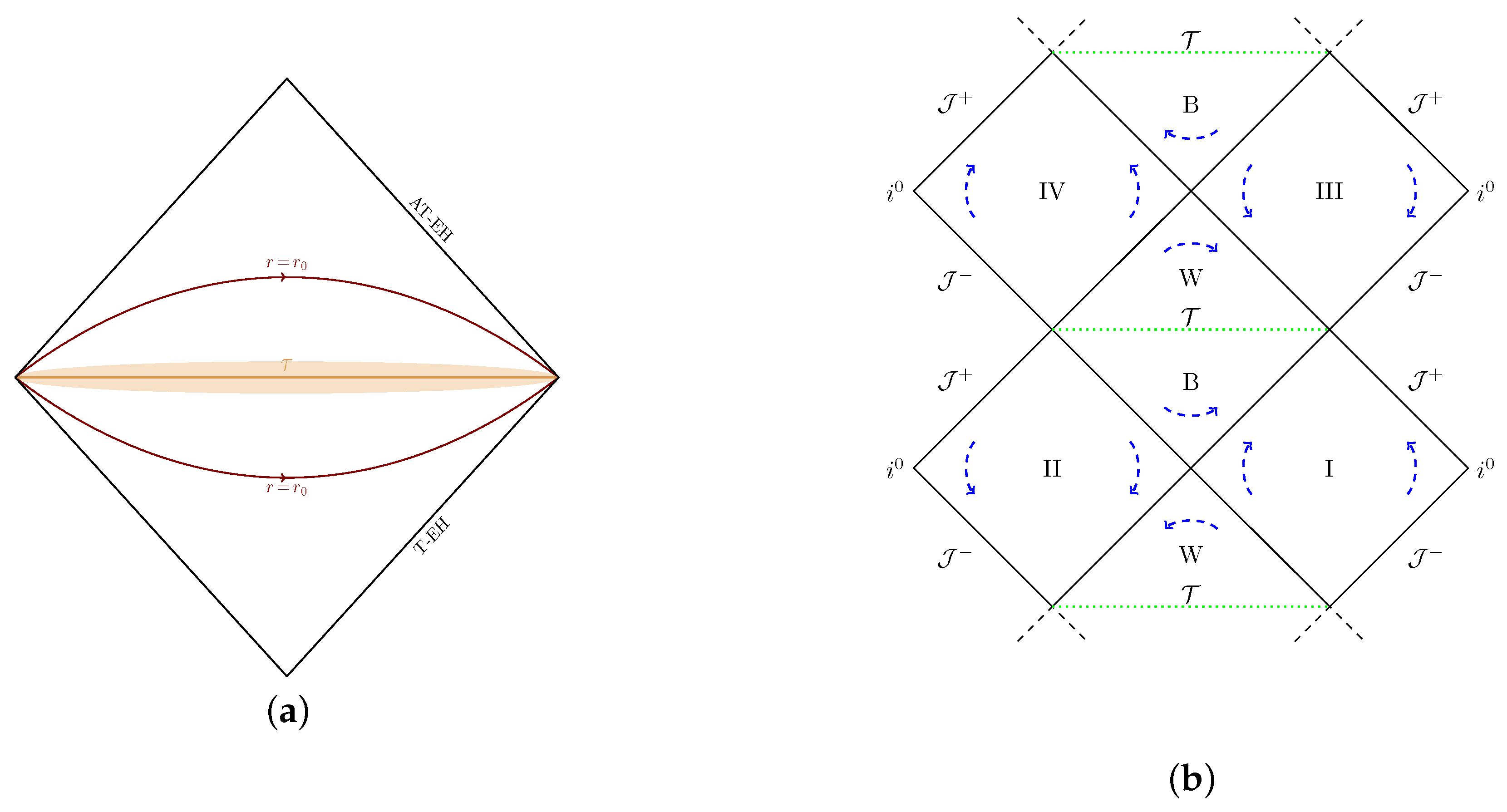
(1) Dynamical horizons: what forms and evaporates is a dynamical horizon [8,9,10,11,12]. There is no null event horizon causally isolating the ‘interior’ region as in Figure 1a. During the formation of the black hole, the trapping dynamical horizon TDH is space-like and the marginally trapped surfaces (MTSs) on it grow in area in the outward direction, while during Hawking evaporation, TDH is time-like and the MTSs shrink in area in the future direction. As we will discuss in Section 2, the absence of an event horizon and growth and shrinking of the TDH are realized in detail in the case of a solvable spherical black hole model.
(2) Non-trivial geometry in the trapped region: already in the semi-classical region, where curvature is much smaller than the Planck scale, the interior space–time geometry develops astonishing features once the back reaction due to the (negative energy) Hawking flux is included. For a macroscopic black hole, the interior geometry evolves very slowly but over an extremely long time. If one introduces a geometrically natural foliation of the interior—say slices with constant values of the Kretschmann scalar, or of the area radius r of round 2-spheres [13,14]—one finds that these slices develop astronomically long necks. (These are the long neck surfaces depicted by the portion LNS of the Cauchy surface of Figure 2b.) Now, partners of the modes that escape to enter the interior of the TDH and evolve on this time-dependent background. One expects that, as in cosmology of the early universe, the astronomical expansion of necks would stretch their wavelengths enormously whence, when sufficient time has passed, the interior of the TDH can house an enormous and increasing number of these modes but with very small total energy. A priori, there is no obstruction to continued entanglement between the modes outside and those inside well beyond the Page time [15].
(3) Singularity resolution: in loop quantum gravity (LQG), the Big-Bang singularity has been shown to be resolved in a robust manner in a large number of models (see, e.g., [16,17]). For the Schwarzschild-interior, there is now an effective description of quantum geometry with several physically attractive features that are hallmarks of the LQG quantum geometry [18,19]. In particular, we again have singularity resolution, there are universal upper bounds on curvature invariants, and the quantum modifications of Einstein’s equations die very quickly away from the Planck regime. In the quantum extended space–time, the singularity is replaced by a quantum ‘transition surface’ to the past of which we have a trapped (BH-type) region and to the future of which there is a (white-hole type) anti-trapped region1 (see Figure 2b). In this scenario, the quantum extension of space–time has an asymptotic region with . The extremely long wave-length modes inside the T-DHs—that are entangled with those emitted to —travel across the transition surface to the anti-trapped region and then leak out slowly to on a time scale ≳ [20]. Thus, the correlations between outgoing modes (with an ‘approximately thermal’ character) that were emitted in the ‘Hawking phase’ of quantum radiation and their partners can be restored on but on a much longer timescale.
Each of these three ideas constitutes a major conceptual shift with respect to Figure 1b. Together they provide a more concrete basis for the general, LQG-based paradigm of the black hole evaporation process first proposed in [21], and discussed in a more concrete form in [14]. Section 2 presents the conceptual underpinning of these ideas in greater detail and also discusses further issues that were not included in the summary sketched above. That discussion should make the current status of the program clearer. Similarities and differences with some of the other scenarios [4,5,6,22,23] are illustrated in Section 3. In particular, there is a discussion of issues related to space–time diagrams compatible with geometrical considerations, proposed over the last decade or so (see in particular, [24,25,26,27,28,29,30,31,32]).
2. Black Hole Evaporation: Inclusion of Back-Reaction
In this section, we will expand on the three themes that lie at the heart of the LQG-based paradigm sketched above. Before doing so, however, we need to clarify a preliminary issue that is either implicit or overlooked in most discussions. In Figure 1, the black hole is initially formed by the gravitational collapse of a star. However, the star is generally treated as an “external matter field” in that its constituents do not feature in the black hole evaporation process. Indeed, in Hawking’s original analysis, the black hole evaporates through the emission of quanta of a massless, test scalar field, a field that does not feature in the composition of the star that collapses. Therefore, we do not have a closed system.
However, discussion of unitarity and potential loss of information in the quantum theory requires a closed system. The simplest way to construct such a system to consider only a massless scalar field that is coupled to gravity. Thus, the black hole itself is formed by the collapse of a massless scalar field that is incident from as in Figure 3a, rather than by a star collapse as in Figure 1a. More precisely, in classical GR the incoming state is a narrow pulse of a scalar field—depicted by the shaded null strip—incident from that collapses and forms a black hole. The pulse is chosen to be narrow so we have a prompt collapse and analysis is not excessively contaminated by the details of the pulse profile. It is also chosen to have a ‘macroscopic’ Arnowitt–Deser–Misner (ADM) mass to ensure that classical GR is an excellent approximation in the early stage of the collapse. To the past of the pulse, space–time is flat and, to the future of the pulse, it is isometric to a Schwarzschild space–time. (Sometimes, it is convenient to idealize the situation and consider a Delta-distribution for the pulse profile as in Figure 3b.) In the quantum theory, one is interested in the Hawking radiation of this scalar field. Thus we now have a closed system.
More precisely, in place of the star that originates from past time-like infinity and the incoming vacuum state of a massless test scalar field on that Hawking considered, in quantum theory, we would only have a coherent state of the quantum, massless scalar field, peaked at the classical pulse, and we approximate the collapse using semi-classical gravity until curvature becomes Planckian. Since the quantum fluctuations in a coherent state at are the same as those of the vacuum state, they would again lead to the Hawking process until the black hole shrinks to a sufficiently small mass and quantum gravity proper is needed.
There is, however, one important consideration that has to be kept in mind in the discussion of entanglement. Consider the hypersurface depicted in Figure 2a during the semi-classical phase of the evaporation process. The outgoing modes that go to ‘lie on the portion of ’ that is to the right of the time-like part of T-DH. These are entangled with the entire state that ‘lies on the left portion of ’ which includes both, modes carrying negative energy flux, and the ingoing coherent state. In the literature one often considers entanglement of the outgoing modes only with the negative energy ingoing modes following Hawking’s original calculation in which the collapsing star/field are is included in quantum considerations.
2.1. Dynamical Horizons
Let us begin by recalling the notion of the EH of a black hole. EH is the future boundary of the space–time region from which causal signals can reach . Note that this notion is not only extremely global, but also teleological. Thus, for example, an EH may well be developing in the room you are now sitting in anticipation of a gravitational collapse that may occur in this region of the galaxy a million years from now! Indeed, Figure 3a provides a concrete illustration of how this can happen: the EH forms and grows in the flat part of space–time in anticipation of the scalar field collapse that occurs later. Furthermore, as discussed in a remark below, in models where the back reaction has been analyzed in detail, there is no EH in the semi-classical part of the space–time. It will not materialize in the quantum completion of the space–time if the singularity is resolved. What do we mean by ‘black hole evaporation’ then? Something non-trivial does happen already in the semi-classical part of space–time: as mentioned in Section 1, what forms and evaporates is a dynamical horizon, DH.
A DH is a 3-dimensional space-like or time-like submanifold that is: (i) foliated by 2-dimensional, surfaces S with 2-sphere topology, so that the expansion of one of the null normals to each leaf S is zero and that of the other null normal is either positive or negative everywhere.2 Thus, each S is a marginally trapped surface (MTS). In an asymptotically flat space–time, we can distinguish between the two null normals to S—we will denote by the outgoing null normal and by the ingoing null normal. On a BH type DH, the expansion of the outgoing null normal vanishes (it is positive immediately outside and negative immediately inside the MTS), while the expansion of the ingoing null normal is negative (both outside and inside). Thus, immediately inside a black-hole type DH, both expansions are negative and we have a trapped region. Therefore, we will refer to these DHs as trapping dynamical horizons, T-DHs. One can show that the TDH is space-like when the area of the MTS increases along the projection of on DH, i.e., in the outward direction. More importantly, there is an explicit, precise relation between the growth of the area and the flux of energy (carried by matter and/or gravitational waves) flowing into the horizon: If R is the area radius of MTSs, then [8,9]
where the MTS with area radius is outward relative to that with area radius and (T-DH) is the portion of the TDH bounded by these two MTSs. Thus, not only does the second law of black hole mechanics hold for every TDH but the growth of the horizon area is directly related to the physical process of energy infall. This is in striking contrast with the situation for EHs, where we only have a qualitative statement of growth. Indeed, it is not possible to directly trace the growth to the infall of energy locally because, as we see in Figure 1a EHs can form and grow in flat space–time where there is nothing at all falling across it.
During the evaporation process, by contrast, the MTSs on the TDH shrink, again following (1), and the TDH is now time-like. In the Callen–Giddings–Harvey–Strominger (CGHS) black hole—depicted in Figure 3b—which was analyzed in detail using highly accurate numerical simulations, not only does the TDH exhibit all these features both during the collapse and evaporation, but it has additional properties that have direct physical interpretation. Let me mention two. First, the Hawking radiation starts (in earnest) precisely at the (retarded) instant of time at which the TDH has maximum area. Second, as the evaporation proceeds, the area of the TDH at any time instant is directly related to the Bondi mass at the corresponding retarded time instant at [33,34,35,36].
Finally, let us consider white-hole type DHs. Now, it is the expansion of the ingoing null normal that vanishes and the expansion of the outgoing null normal is positive. Thus, immediately inside these horizons, both expansions are positive: we have an anti-trapped region. We will, therefore, refer to these horizons as anti-trapping dynamical horizons (AT-DH). Since it is that vanishes on any AT-DH, it is natural to investigate what happens to the area of the MTSs as one moves along the projection of on the AT-DH. If the AT-DH is space-like, its area decreases (now in the inward direction) and if it is time-like its area increases (now in the future direction).
Thus the main differences between EHs and DHs are the following. First, EHs refer to the global structure of space–time and are teleological, while DHs can be located quasi-locally and their properties have a direct relation to physical processes at their location. Second, EHs is null while DHs can be space-like or time-like, and become null only when they become ‘isolated’ i.e., there is no flux of energy across them. Third, nothing can ever escape to the ‘exterior’ region from the trapped region enclosed by a BH-type EH and nothing can ever enter the anti-trapped region bounded by a WH-type EH. While there are trapped surfaces immediately inside a T-DH, one can send causal signals across a TDH from inside to outside (see Figure 2b and Figure 4b). Similarly, there are future-directed causal curves that traverse an AT-DH from outside to inside.
Remark: As emphasized by Geroch and Horowitz [37], for the notion of an EH to be useful in discussions of black holes, it is essential that be complete; otherwise, even Minkowski space could have an EH! I mention this caveat explicitly because it is often overlooked in the discussion of information loss. Consider the gravitational collapse of a shell depicted in Figure 3. In the classical theory, there is indeed an EH formed by the (thick) shell collapse because is complete and the EH is the future boundary of the causal past of (see Figure 3a). However, the situation changes when the back reaction is included. The evaporation process has been studied in detail for the CGHS black hole in the semi-classical regime (see in particular [33,34,35,36]) and concrete ideas have been put forward for how the semi-classical discussion can be completed in quantum gravity [38]. This evaporation process of is depicted in Figure 3b. The singularity persists also in the semi-classical space–time (although it is milder in that the space–time metric is now continuous across the singularity). Therefore the semi-classical space–time has a future boundary depicted by the ‘last ray’ in Figure 3b. It is tempting to interpret it as the EH. However, one can check explicitly that of this semi-classical space–time is incomplete and therefore the last ray is not a portion of an EH [34].3 Indeed, the semi-classical part of the quantum space–time has no event horizon at all: what forms and evaporates in this space–time is a T-DH.
2.2. No Violation of Semi-Classical Expectations
Consider the space–time depicted in Figure 2a governed by the coupled semi-classical gravity equations
and the state of , depicting a prompt collapse of a (thick) shell of the scalar field incident from , depicted by the shaded region in the figure. The collapse gives rise to the formation of a space-like T-DH, shown by the left part of the (dark) line labeled TDH in the support of the collapsing scalar field. This part starts with zero area (at the top left corner) and the area of MTSs continues to grow rapidly (in the outward direction) as long as there is incoming flux of (positive) energy carried by the scalar field. If we were to ‘switch-off’ quantum effects, then the situation would be as in Figure 3a: Once the incoming energy flux terminates, this TDH would smoothly join on to a null isolated horizon—the future part of EH. The singularity would stretch all the way to . However, because of quantum effects, the fluctuations in the incoming coherent state give rise to spontaneous (and stimulated) emission. Modes are created in pairs, one going in, and the other going out to . There is thus a flux of negative energy into the ‘interior region’ whence, in contrast to the classical theory, the TDH does not become a null isolated horizon. Instead, it becomes null only instantaneously and continues as a time-like 3-surface as depicted in the right branch of TDH in Figure 2a. As the negative energy flux across this portion of the TDH continues, the area of MTSs on this portion of the TDH decreases. Recall, however, that by assumption the ADM mass of the system is ‘macroscopic’—say a solar mass, . Then initially, the ingoing flux is very small and, correspondingly, the area also decreases very slowly. Indeed, the radius starts out at ∼3 km (corresponding to the dynamical horizon mass ) and to reach, say, ∼0.1 mm (so that the now equals lunar mass, ), it takes some years!
For concreteness, in this subsection we will focus on this phase of evaporation, during which a solar mass shrinks to a lunar mass T-DH. Now, during this long process there is no a priori reason to expect a violation of semi-classical considerations because we are very far from the Planck regime throughout this slow transition. However, this premise does violate an intuition based on considerations of the ‘Page time’ [15] that many in the community rely on. Our strategy is to assume that semi-classical considerations are valid for reasons just mentioned, and see if one runs into roadblocks that force us to concede that the assumption is incorrect.
Calculations have been carried out in some detail within the semi-classical framework to support the scenario I summarize and I believe that it is possible to make the entire analysis rigorous (say by Phys. Rev. D or J. Math. Phys. standards) using quantum field theory in curved space–times to analyze in greater detail the behavior of partner modes in the dynamical background space–time. Pairs of Hawking modes are created continually during this long process, one going to infinity and its partner falling inside the time-like portion of the T-DH. These modes will be entangled whence, if one uses the usual observable algebra based just at , the state would seem mixed, close to a thermal state. (For caveats on departure from thermality, see, e.g. [40]). When will the correlations be restored? For this to happen, the partner modes would have to emerge from the trapped region and propagate to .
Now, one’s first reaction could be that this ‘purification of the state’ could occur continually throughout the -year long process because there is no causal obstruction for the modes that entered the trapped region bounded by the TDH to come out across its long time-like portion. Indeed arguments have been made to say that there is no information loss issue at all because there is no event horizon and fields can escape across the time-like TDH (see, e.g., [41,42]). But in semi-classical gravity, throughout this process partners of modes that go out to continue to fall into the trapped region; they do not come out. So the fact that there is no causal obstruction for the partner modes to emerge from the trapped region does not by itself lead to purification in the semi-classical space–time.
Furthermore, there is an important puzzle. During the long process, a ‘very large number of modes’ has escaped to infinity (some by a back of the envelope heuristic counting). But the horizon mass is now the lunar mass, , only about times . In terms of modes then, those that escaped to infinity have carried away almost all the initial and their partner modes have only . Therefore, at the end of the semi-classical process under consideration, one would have to have a huge number of modes carrying a total of in energy to , and the same number of modes inside the TDH with a minuscule mass. How can a TDH with just a mm radius accommodate all these modes? Even if we allowed each mode to have the (apparently maximum) wavelength of mm, heuristically one would need the horizon to have a huge mass—some times the lunar mass! While these considerations are quite heuristic and the semi-classical calculations are much more precise, one needs to face the conceptual tension: at the end of the process under consideration, the TDH has simply too many modes to accommodate, with a tiny energy budget. Is this not an indication that, contrary to what semi-classical considerations suggest, most of the ‘purification’ must have occurred by the time the TDH has shrunk down to the lunar mass? That, as is often argued, ‘purification’ must begin already by Page time [15] when the TDH has lost only half its original mass of ? If so, semi-classical considerations must fail even for macroscopic black holes; there must be unforeseen quantum effects which get us out of this quandary.
This does seem like a serious problem with the original assumption on the validity of the semi-classical theory for the process under consideration till one takes a more careful look at the space–time geometry in the trapped region. It turns out that, because of semi-classical Einstein’s equations, this geometry has some very counter-intuitive features that can resolve this quandary. Calculations of the stress-energy tensor on the Schwarzschild space–times confirm the idea that in semi-classical gravity there is a negative energy flux across the time-like portion of such that would decrease according to the standard Hawking formula: . Indeed, this is the basis of the standard view that the evaporation time goes as . One can then argue that, in the phase of evaporation under consideration, the form of the space–time metric in the region bounded by the of Figure 2a is well approximated by the Vaidya metric:
with . (This is because during this phase the quantum correction to the Schwarzschild metric of classical GR are small.) In particular, an analogous conclusion is borne out in the detailed semi-classical analysis of the evaporation of the CGHS black hole. So, let us work with this metric. To understand the nature of space–time geometry it bestows on the trapped region, it is convenient to foliate it by some invariantly defined surfaces. It turns out that the most convenient choices are [13]: and where r is the area radius of the round 2-spheres and is the Kretschmann scalar:
where the last equality expresses the value of the Kretschmann scalar in the Vaidya metric. (Note that it has the same form as in the Schwarzschild space–time, with the constant m of the Schwarzschild space–time replaced by ; derivatives of do not appear!) A typical leaf of these foliations is represented in Figure 2 by the portion of the Cauchy surface that lies in the trapped region, the left end of the leaf lying on the space-like portion of TDH and the right end on the time-like portion.
If we were to ignore the quantum radiation as in Figure 3a depicting the scalar field collapse in classical GR, would be constant, the metric in the trapped region would be just the Schwarzschild metric and both foliations would coincide, each leaf being the standard homogeneous slice in the Schwarzschild-interior. However, because of quantum radiation is a monotonically decreasing function of v and the two foliations are distinct. If we consider the full trapped region (beyond the semi-classical part discussed in this sub-section), the foliation is conceptually better suited to separate the transition between the part where semi-classical considerations provide an excellent approximation, and the part where curvature enters the Planck regime and corrections from full quantum gravity becomes crucial. However, while each leaf is space-like almost everywhere starting from the left end, it becomes null extremely close to the right end. Thus each leaf has a time-like portion, albeit extremely tiny. The foliation, on the other hand, is space-like everywhere and easier to visualize. However, this foliation does not cleanly separate the trapped region into a part on which semi-classical considerations provide an excellent approximation and part where corrections from quantum gravity properly become important. Thus, each has its merits and it is appropriate to consider both these foliations. Both provide a foliation of the entire trapped region of Figure 2a.4
Geometry of the leaves of these foliations can be analyzed simply by pulling back the space–time metric (3) to them. Each leaf is topologically and is itself foliated by round 2 spheres which can be labelled by values of the advanced time coordinate v. Let us set when , and when it reaches the lunar mass , both at the right end, i.e., on the time-like portion of the T-DH. Thus, the radius of the MTSs decreases from Km to mm. In both foliations, as v increases the leaves develop longer and longer necks of length along the directions (while the increase in the 2-sphere radius is much less pronounced). The ‘final leaf’ for the process under consideration in this sub-section starts at the right end with where equals . For the two foliations under consideration, the length of the final leaf is given by:
where ‘lyr’ stands for light years. The radius of 2-spheres is constant, cm on this entire leaf for the foliation, and increases from cm to cm from the right to the left end for the foliation. Thus, during the slow evaporation process, the leaves develop astronomically long necks!
The dynamical nature of the intrinsic geometry of these leaves suggests that the partner modes that fall across the time-like part of the TDH will get enormously stretched during evolution from to , as in quantum field theory on an expanding cosmological space–time, and become infrared. As I mentioned, a back of the envelope calculation suggests an enormous number—some —of these partner modes is created during the long process during which the black hole shrinks from a solar mass to a lunar mass! But with such infrared wavelengths, it is easy to accommodate them in the trapped region with the energy budget only of . Thus, even though the outgoing modes carry away mass to , there is no obstruction to housing all their partners in the trapped region on a slice of Figure 2a with the small energy budget of just . This argument removes the necessity of starting purification by Page time. In the LQG perspective of this article, purification can be postponed to a much later stage.
Of course, these considerations need to be made precise using quantum field theory on the Vaidya space–time of Equation (3). In particular, while the qualitative phenomenon of the ‘stretching of the wave-length’ is familiar from the theory of cosmological perturbations in the inflationary epoch, the process and the associated energy considerations need to be spelled out using renormalized stress-energy tensor of the scalar field . But this is feasible using available techniques form quantum field theory in curved space–times by exploiting spherical symmetry. Indeed, in the semi-classical region under consideration in this sub-section, the space–time metric can be viewed as a perturbed Schwarzschild-interior—or the Kantowski–Sachs—metric. Finally, although the foliations discussed above are geometrically natural, from a covariant perspective, one may have reservations about using any foliation at all. However, one can think of these foliations simply as mathematical tools that provide us intuition to help answer invariantly defined questions, as is commonly done in cosmological contexts.
2.3. Singularity Resolution and the Quantum Region
The question remains, of course, as to how purification is to occur at a later time. Now, if the space–time geometry in the entire trapped region were to be given by the Vaidya metric, a space-like singularity would constitute the future boundary of the trapped region (as in, e.g. [32]). Then in our scenario, there would be no chance for all the partner modes to escape to and restore correlations with the modes that reached during the long semi-classical phase (i.e., by the retarded time , defined by the last ray in Figure 2a). Thus, purification can occur only if the space-like singularity of the Vaidya metric is resolved because the quantum geometry in the Planck regime is qualitatively different and singularity-free. Can LQG quantum geometry naturally resolve the singularity? In this subsection, we will address this issue in two steps. In the first, we will recall some results on the resolution of the black hole singularity in the non-dynamical Kruskal space–time. In the second we will summarize the current expectations for singularity resolution for the dynamical space–time now under consideration, in which the trapped region results from the gravitational collapse of the quantum scalar field , and there is further quantum dynamics because of creation of the Hawking pair of modes that react back on the space–time geometry.
2.3.1. Kruskal Space–Time in Lqg
Recall that the big-bang singularity of Friedmann–Lemaitre–Robertson–Walker (FLRW) space–times are naturally resolved by the quantum geometry effects of LQG (see, e.g., the review articles [16,17]). The big-bang is replaced by a big-bounce, to the past of which we have a contracting phase and to the future of which we have an expanding phase. Space–time curvature reaches an universal upper bound at the big-bounce. Recall that at the big-bang the radius of space–time curvature vanishes, while in Minkowski space–time . In loop quantum cosmology (LQC) of FLRW models, the radius of curvature has an absolute lower bound . Now, the trapped region of the Kruskal space–time—often called the Schwarzschild-interior in the literature—is isometric with a Kantowski–Sachs metric, which is foliated by homogenous slices, each with topology . Therefore, over the years LQC techniques were applied to the interior to probe the issue of singularity resolution (see, e.g., [45,46,47,48,49,50,51,52,53,54,55,56]). However, because the Kantowski–Sachs space–time is anisotropic—and furthermore anisotropies are technically different from those of the better understood Bianchi models [16,17]—progress has been slower. While the LQC quantum equations can be written down also for the Schwarzschild-interior, only the effective equations have been solved in detail. These provide a quantum corrected effective metric for the Schwarzschild-interior—a smooth tensor field that shares the isometries of the Schwarzschild metric but with coefficients that involve the Planck length . The black hole singularity is resolved in all investigations but details of quantum modifications differ. For brevity, I will restrict myself to one [18] which is free of all the known drawbacks (for a detailed comparison of quantum modifications, see [19]).
As Penrose has emphasized over the years, there are key structural differences between the FLRW and Schwarzschild singularities in classical GR because in the first case it is the Ricci curvature that diverges while in the second case it is the Weyl curvature. While there are ‘normal’ 2-spheres arbitrarily close to the big-bang (with ), every 2-surface in the region near the Schwarzschild singularity is trapped (with ). Therefore, there are some important differences also in the quantum theory. However, rather unexpectedly, there are also close similarities. I will present a few illustrations while discussing the singularity resolution in the Schwarzschild-interior.
The main features of the singularity resolution can be summarized as follows. As depicted in Figure 4a, the Schwarzschild singularity is replaced by a (space-like) transition surface in LQG. To the past of we have a trapped region, expansions and of the two null normals and to the round 2-spheres are both negative. Both expansions vanish on and become positive to the future of . Thus, we have an anti-trapped region to the future. The radii of round 2-spheres decrease as we approach from below and increase as we move upwards. Therefore the radius attains its minimum value at . This is analogous to the fact that the scale factor a attains its minimum value at the LQC big bounce in FLRW models.5 Also, curvature attains its maximum value at the transition surface, and that value is universal (for macroscopic ADM masses assumed in obtaining effective equations). For example, the Kretschmann scalar is given by:
where is a numerical constant and is the area gap of LQG, and M the ADM mass of the Schwarzschild space–time under consideration. This corresponds to a universal minimum, , for the curvature of radius in the LQG extension of the Schwarzschild-interior. In the FLRW model, curvature attains a universal upper bound at the bounce surface and the corresponding lower bound for the curvature radius is . Thus, rather surprisingly, the minimum values are the same within a factor of although the structure of singularities and the detailed analyses leading to these values are very different. Next, in the LQC of FLRW models, quantum geometry corrections decay rapidly away from the bounce. The same is true in the Schwarzschild-interior, as one moves away from the transition surface . For example, even in the case when , the quantum geometry corrections at the horizon are less than 1 part in . So, the geometry is well approximated by the Schwarzschild solution until one reaches a small neighborhood of . Thus, even a black hole with mass as low as qualifies as a ‘macroscopic’ in this effective theory.
A major difference between FLRW models and the Schwarzschild-interior is that in the classical theory it is the presence of matter that gives rise to non-trivial curvature in the former, while there is no matter in the latter. In both cases, singularity is resolved because the left-hand side—i.e., the geometrical part—of Einstein’s equations receive corrections due to LQG quantum geometry. In the FLRW case, one can manipulate the effective equations and interpret the new terms as corrections to the matter part in the Friedmann and Raychaudhuri equations. Then the LQC corrected Friedmann equation, for example, reads [57]
being a numerical constant. Thus the area gap is the microscopic LQG parameter that dictates the macroscopic parameter which determines the regime in which LQG effects are important. The negative sign in front of the quantum correction implies that effective energy density is lower than in the classical theory, but the negative quantum contribution becomes quickly negligible away from the Planck regime. In the Planck regime, however, it creates a very large effective repulsive force that is responsible for the resolution of the big-bang singularity. In the case of Schwarzschild-interior the mechanism is similar and can be seen even more directly. In the classical theory, and curvature resides entirely in the Weyl part. But because of quantum geometry effects, is no longer zero in the effective theory and one can choose to interpret it as an effective stress-energy tensor induced by quantum geometry. For macroscopic black holes, one finds that the invariant is negligible near the horizon but increases very rapidly near , reaching the Planck scale value at , and then decreases rapidly again in the anti-trapped region. The effective stress–energy tensor has the form of the stress-energy tensor of a perfect fluid. As one would expect, the corresponding energy density and pressure are negative. Just as the negative sign in front of the quantum correction to the Friedmann equations arises naturally from the LQG quantum geometry without additional inputs, the negative sign of the effective energy density and pressure arise naturally. They are responsible for an effective repulsive force that leads to the singularity resolution. It is again quite surprising that while the negative energy density becomes sufficiently high in the Planck regime to avoid a curvature blow up, it dies very quickly away from the Planck regime. Figure 4b shows the LQG extension of full Kruskal space–time [19]. It is included only for completeness. Just as the full Kruskal space–time is not directly relevant to a black hole formed by gravitational collapse or to discuss its evaporation, only a part of this picture is relevant for our present discussion. The relevant part is shown in Figure 2b which we now discuss.
2.3.2. Beyond the Semi-Classical Region
When do quantum gravity effects become important? Consider as an example the closed FLRW model. In this case, the notion of the volume of the universe is unambiguous. Sometimes it is said that quantum effects become important only when the universe contracts to the Planck size, i.e., when its volume is given by . However, detailed calculations have shown that this is not the case: What matters is when the curvature reaches the Planck size; not the volume [58]. In a solution in which the universe grows to a maximum radius of a megaparsec, for example, a bounce occurs when the volume of the universe is . Thus, in this solution, quantum gravity effects completely dominate the dynamics when the universe is the size of a small mountain, and it never gets smaller. This is because in LQC the curvature reaches its maximum allowed value already at this stage. The situation is the same in the case of a black hole: what matters is the curvature. Consider the shell collapse, depicted in Figure 3a. For a solar mass Schwarzschild black hole, the curvature becomes Planckian already when the shell reaches radius , whence quantum gravity effects can dominate the dynamics already at this stage.
In semi-classical considerations of Section 2.2, we restricted ourselves to a time interval , during which the mass of the TDH decreases from the solar mass, , to the lunar mass, , to first bring out and then resolve an apparent problem already in this very tame regime. But one would expect the domain of semi-classical approximation to be much larger, say till the space–time curvature becomes . Let us then consider the corresponding surface within the trapped region. At the left end of this surface we encounter the infalling shell whose radius has shrunk to . At the right end of this surface, i.e., on the time-like portion of T-DH, we would have , so that the corresponding dynamical horizon mass is . This 3-surface—depicted by the past boundary of the shaded region around the transition surface of Figure 2b—is the future boundary of the semi-classical part of the trapped region. We will denote it by . In the trapped region, we can trust the semi-classical approximation of Equation (2) to the past of but not to its future.
To discuss the space–time and scalar field dynamics to the future of , we need to consider interaction between the quantum scalar field and quantum geometry. In Figure 2b, the portion of space–time in which one has to go beyond semi-classical approximation is depicted by the (pink) shaded region around the transition surface (together with a (red) blob at the right end). Let us divide the problem into two parts by slicing this region by 3-surfaces, so that we have at the left end, which then decreases as we move to the right. Since the negative energy flux is very small over a very large time span, one would expect the quantum geometry to change very slowly during this phase. As discussed below, we should be able to describe dynamics during this phase using certain adiabatic approximations. At the end of this adiabatic phase, however, one would need full quantum gravity. The region where this will be necessary is depicted in Figure 2b by the (red) blob at the right end of the transition surface .6
To describe dynamics during the adiabatic phase we can seek guidance from other areas of physics. Consider propagation of light—the quantum Maxwell field—in a medium, say water. The medium itself is in a quantum state of a large number of molecules, and, at a fundamental level, we need to consider the interaction of photons with these molecules. However, so long as the photon beam is not so strong as to alter significantly—they do not, e.g., boil the medium—the photons do not see the details of quantum fluctuations of molecules. The propagation can be well-approximated by computing just a couple of numbers—the refractive index and the birefringence—from and then characterizing medium just by these two parameters.
The same strategy has been used in LQC. For concreteness, let us consider the the tensor modes of cosmological perturbations, represented by quantum fields , (with ). At a fundamental level, they propagate on the background FLRW quantum geometry, described by a wave function where is the inflaton. That is now evolve on a probability distribution of smooth classical FLRW metric , rather than on a single . But it turns out that so long as the back reaction of these perturbations is negligible, their propagation on the quantum geometry is extremely well approximated by their propagation on a smooth metric , constructed from [59], is called the dressed effective metric.7 (Thus, the coefficients of depend on ℏ.) As with the propagation of photons in a medium, this is possible because the cosmological perturbations do not see all the details of quantum fluctuations in and the information they do see is captured in .
One would expect a similar result to hold during the adiabatic phase of black hole evaporation now under consideration since the change in the background curvature occurs very slowly. During this phase, the quantum state of geometry can be taken to be sharply peaked around a smooth metric, and the propagation of the partner modes of the scalar field on this quantum geometry should be well approximated by their propagation on a smooth dressed effective metric , constructed from . As in the two examples discussed above, the partner modes will not be sensitive to all the detailed quantum fluctuations in and the information they do see will be captured in the dressed effective metric which is smooth but inherits ℏ-dependent terms from . There is a conceptually streamlined procedure to find this metric. Note that this would likely be more refined than the effective metric in the LQG description of Kruskal space–time discussed in Section 2.3.1, as it will likely incorporate some of the quantum fluctuations in geometry and the scalar field that are not registered in the effective metric.
Thus, the study of dynamics in the full trapped region can be divided into three phases:
- (i)
- A semi-classical phase which is expected to provide an excellent approximation to full quantum dynamics in the part of the trapped region that lies to past of the surface . This is the part of the trapped region to the past of the shaded (pink) portion in Figure 2b. During this phase dynamics would be well approximated by quantum field theory of the field on the Vaidya background. During this phase, space–time
- (ii)
- An adiabatic quantum gravity phase in which the space–time curvature is larger and enters the Planck regime but the evaporation process is adiabatic. This phase, depicted by the shaded pink region of Figure 2b, could be well-described by a dressed effective metric . The task is to calculate this and use it to describe the propagation of the field . This region is expected to constitute a neighborhood of the transition surface, , to the past of which we have a trapped region and to the future of which, an anti-trapped region, both defined using . The metric will incorporate two distinct sets of quantum effects. The first set is from LQG proper—such as negative effective energy density which is very large in the Planck domain and reduces the mass of the infalling scalar field enormously even at the left end, , of the shaded (pink) region, even though the influx of the Hawking partner modes is negligible there. As v increases, we slide to the right in this region, and then the negative energy density due to quantum geometry effects decreases but is compensated by the negative energy carried by more and more partner modes. The second set of quantum effects is precisely that from the dynamics of the scalar field. It includes both, the evolution of the incoming shell and the infalling partner modes. The actual calculation will incorporate both these types of effects in one go. But conceptually it is useful to separate the two contributions, since the first has been absent in most other approaches as they focus just on the partner modes and also ignore the quantum geometry effects. Finally, the Kruskal results depicted in Figure 4a suggest that the first set of effects will decay rapidly as we move away from Planck curvature into the semi-classical region. Therefore in the semi-classical region, will be well approximated by the semi-classical Vaidya metric used there.
- (iii)
- A full quantum gravity phase that is localized in the region depicted by a dark (red) blob at the right end of the shaded region in Figure 2b. This is the region in which not only is the curvature of Planck scale, but it is varying rapidly because of the evaporation process; dynamical nature of the back reaction is now significant. Therefore, description in terms of would now be inadequate. In this phase, one would have to use the LQG quantum state for the combined system, adapted to the spherical collapse under consideration. In terms of space–time geometry, the time-like piece of TDH continues to shrink in the semi-classical region and terminates in the full quantum region as depicted in Figure 2b.
Next, consider the untrapped region to the future of the transition surface , defined by the dressed effective metric . Experience with effective equations in the Kruskal extension suggests that the untrapped region will end, its future boundary being an anti-trapping dynamical horizon, AT-DH (see Figure 2b). As time evolves, the infrared modes in the trapped region will cross and eventually escape to infinity. Therefore, there would be an outward flux across AT-DH. Considerations of Section 2.1 then lead us to the conclusion that AT-DH will be space-like, with its area shrinking in the direction of the projection of on AT-DH, i.e., in the inward direction. Finally, recall that the radius r of 2-spheres achieves its minimum on the transition surface , since it increases as we move away from in both future and past directions. Using this fact, one can argue that the anti-trapping horizon AT-DH will emerge from the fully quantum region and then move left, shrinking in its area and eventually plunging into at its left end, achieving minimum possible area. Note incidentally that the space–time geometry is far from being symmetric around the transition surface. In particular, while the mass of the time-like piece of TDH decreases from to some ∼100 , the mass decreases from ∼100 to, say, . However, this asymmetry is present—albeit to a much smaller extent—already in the LQG extension of Kruskal space–time [19] discussed in Section 2.3.1.
Finally, the region to the future of AT-DH would also be well approximated by a Vaidya metric, but now the outgoing one, expressed in terms of the retarded time coordinate u in place of the advanced time coordinate v of Equation (3). It will describe the propagation of the infrared modes that will emerge from the AT-DH and arrive at at very late times. General considerations by Ori [20], and Bianchi et al [29,31] suggest that the time scales associated with this process will be long, .
2.4. Summary: The Global Picture
Let us summarize the discussion of the last three sub-sections. One begins with a coherent state of a quantum scalar field , peaked around an infalling classical pulse on , undergoing a ‘prompt collapse’. In the initial stages of the collapse, space–time is well approximated by classical GR where space–time is flat to the past of the support of the pulse, and Schwarzschild to the future, as depicted in Figure 3a. When the radius of the (thick) shell has become sufficiently small, a trapping dynamical horizon TDH forms. In classical GR of Figure 3a, TDH has only a space-like component. In the quantum theory, it has two components as shown in Figure 2a. The inner component is space-like, (essentially) the same as in the classical theory, while the outer component is new; it replaces the event horizon EH of Figure 3a. However, it is time-like, rather than null, and decreases in area due to the negative energy flux of the Hawking ‘infalling partner modes’ as in Figure 2a.
The two branches of the TDH serve as the past boundary of a trapped region. Figure 2a shows the part of the evolution during which semi-classical approximation of Equation (2) holds. As discussed in Section 2.2, during this very long phase of evolution, the mass of the time-like part of the TDH shrinks from the ADM mass, , to . Pairs of modes are created, one going to infinity and the other falling into the trapped region. The outgoing modes carry away almost all the initial mass to and the radiation is approximately thermal there. Thus the Bondi mass at when the last ray from the semi-classical region reaches is only of the order of . However, the outgoing modes are entangled with the infalling ones. While the total quantum state of the system is a functional of both the geometry and the scalar field, geometry is well-approximated by a solution to Equation (2) in this semi-classical phase; it can, therefore, be taken to be a smooth metric. Thus, one can focus just on correlations between the (observables associated with the) scalar field in the untrapped region and the trapped region on a Cauchy surface, such as of Figure 2a. Note, however, that the trapped region includes not only the partner modes but also the infalling coherent state. The mass associated with the outgoing modes is , which is huge if u is taken to be sufficiently late so that is still macroscopic but much smaller than . In Section 2.2, as a concrete example, we took to be the solar mass and to be the lunar mass . Then mass associated with the part of the state in the trapped region is only times the mass associated with the outgoing modes. Therefore, there is an apparent tension: How can the trapped region house the same number of partner modes as those that went out to with a tenth of a million in energy budget? Alternately, since the radius of (the time-like branch of) TDH has shrunk to cm (corresponding to the ), how can so many modes reside in an apparently tiny region? As we saw in Section 2.2 the answer lies in the fact that although the radius at the TDH is tiny, restriction of the Cauchy surface to the trapped region has an astronomically long neck— light years if is taken to be surface in the trapped region, and light years if it is a surface. Therefore the scalar field modes would be enormously stretched and become infrared, each carrying such a tiny energy that the small energy budget can be easily accommodated. I believe that these considerations can be significantly sharpened using quantum field theory on the Vaidya background in the trapped region.8
To the future of the semi-classical region, curvature can exceed , whence we need quantum gravity. To describe this phase of dynamics, we are guided by two considerations: the quantum corrected, effective LQG equations describing Schwarzschild-interior (discussed in Section 2.3.1), and suitable approximations during the phase in which quantum geometry changes adiabatically (mentioned in Section 2.3.2). The effective LQG equations imply that the Schwarzschild singularity is resolved and replaced by a transition surface , to the past of which we have a trapped region and to the future, an untrapped region. Curvature is bounded above and reaches its upper bounds on . Experience with other systems—such as the propagation of the quantum electromagnetic field in a medium, or, of cosmological perturbations on the quantum FLRw geometry—suggests that so long as the evaporation process is adiabatic, i.e., the mass loss is not too fast, one should be able to introduce a smooth metric that captures all the information in the quantum state of geometry that is seen by the evolving scalar field . We are primarily interested in this evolution in order to determine whether the correlations between the early time outgoing and infalling modes are ultimately restored.
Thus, the quantum evolution to the future of the semi-classical region can be divided into two parts: (i) an adiabatic quantum gravity phase in which we continue to have a slowly varying smooth metric that dictates dynamics of ; and (ii) a full quantum gravity phase in which we have to use the full quantum state that is now a functional both of geometry and the scalar field. The first of these two phases lasts very long as indicated by the shaded (pink) region in Figure 2b, while the second phase is short, as indicated by a dark (red) blob on Figure 2b. There is a systematic procedure to analyze the adiabatic phase in detail and this task can be undertaken soon. Analysis of the full quantum gravity phase is the hardest of open issues since it will involve full LQG as applied to this model. However, it seems reasonable to assume initially that the major effect of this full quantum region on future evolution would be in the region bounded by the two null rays and of Figure 2b. Under this hypothesis, one can solve for dynamics in the rest of space–time and see if the expectations about purification at late times are borne out.
Specifically, the proposal is that there will be a transition surface, , now in the geometry defined by , separating a trapped and an anti-trapped region. The anti-trapped region will be bounded in the future by an anti-trapping dynamical horizon AT-DH (see Figure 2b). The infrared modes with a very small total energy will leak out across AT-DH and propagate to . The geometry to the future of this AT-DH will be well approximated by the Vaidya metric in the retarded Eddington–Finkelstein coordinates . All along, these modes will be entangled with those that reach before in Figure 2b. Therefore purification will occur at late times. Detailed calculations should reveal if the correlations will be (in essence) fully restored, or if the influence of quantum region between and plays a major role in this purification process. There is a suggestion in LQG [61] that the ultraviolet structure of quantum geometry may trap some correlations. The above discussion suggests that the infrared modes will carry significant or almost all correlations but does not rule out the possibility of trapping some correlations in the quantum region.
Analysis of the fully quantum region is the most difficult of open problems. One promising approach is to generalize the analysis of [62] in which the quantum evolution across the singularity of a 2-dimensional black hole was studied. But the required generalization would be quite non-trivial. One may, therefore, ask: is the ‘full quantum gravity phase’ essential? It is true that the arguments that enable one to describe quantum geometry using break down in this region. But could we not perhaps introduce other arguments and describe the entire quantum gravity phase in terms of some smooth metric with coefficients that depend on ℏ? Is there an obstruction for such a metric to exist? Detailed considerations involving the transition surface, the behavior of the area radius r, and the nature of the trapping and anti-trapping horizons—TDH and AT-DH—of Figure 2b imply that such a metric cannot exist in the entire quantum gravity region within the paradigm we have sketched. A ‘fully quantum gravity phase’ is necessary also from the perspective of radiation at . During the semi-classical phase, as the TDH shrinks, the temperature associated with the radiation at grows and more and more short wavelength modes are received. On the other hand, the radiation that emerges from the anti-trapped region has extremely long wavelengths at . A ‘fully quantum gravity phase’ may play an essential role in understanding this dramatic transition. Thus, there are three seemingly independent considerations that lead one to the conclusion that there must be a genuine quantum gravity region denoted by a (red) blob at the right end of : failure of the adiabatic behavior towards the end of the evaporation process, geometric considerations near the transition surface, and dramatic change in nature quantum radiation at .9
3. Discussion
As in most of the investigations of the issue of information loss in LQG, the conceptual underpinning of the program summarized here can be traced back to a general paradigm [21], inspired by the natural resolution of singularities of GR in LQG. This paradigm is based on two observations: (i) one needs to shift emphasis from event horizons to dynamical horizons; and, (ii) if the singularity is resolved, quantum space–time would not end where the classical singularity occurred, whence there is ‘more room’ for the restoration of correlations. While the paradigm opened an avenue for this restoration, it did not provide a detailed mechanism. Developments in subsequent years have helped construct the mechanism. First, we now have detailed analyses of the space–time geometry in the trapped region of a black hole resulting from the gravitational collapse of a null, thick shell, incident from [13,43,44]. Second, we have a much better understanding of the causal structure of the LQG extension of the Schwarzschild-interior [18,19]. The program outlined in Section 2.4 incorporates these developments and outlines concrete steps that are needed to address the issue of whether correlations are restored at .
There is vast literature on the issue of information loss. So I will focus only on those investigations that are directly relevant to the issues discussed here and compare and contrast them with the ideas discussed in Section 2. First, as mentioned in Section 1, there are approaches in which one does not expect singularity resolution. For example, using the AdS/CFT conjecture it has been argued that the Schwarzschild-like singularities will not be resolved in string theory [23]. If this is indeed the case, then one would be led to a space–time diagram like Figure 1b. As already remarked, I share the general consensus in the GR circles that in this case the evolution from to will not be unitary and correlations will be lost. Generally, the string theory literature considers black holes in the presence of a negative cosmological constant as a simplified mathematical context to probe what would happen in the asymptotically flat case of direct physical interest. However, the arguments tend to make strong use of the asymptotically anti-de Sitter boundary conditions and it is far from being obvious how they would then extend to the case of direct physical interest. Indeed, it is not often that one finds space–time diagrams analogous to Figure 2b that explicitly provide the hoped-for purification mechanism in the asymptotically flat context.
However, discussions motivated by the AdS/CFT considerations do have a key point in common with the LQG based ideas: It is expected that correlations will be restored and the S-matrix would be unitary. There is a possibility that the singularity is resolved but the result is a piece of space–time with a new asymptotic region of its own. In such a case, although the information would not be lost globally, it would be lost from the asymptotic region of the part of the space–time in which the collapse occurred [4]. The program discussed here does not favor this possibility but does not rule it out either. This is because of the ‘fully quantum region’, depicted by a dark (red) blob at the right end of the transition surface of Figure 2b. However, as indicated in Section 2.4, the feasible detailed calculations may suffice to reveal whether ‘most’—if not all—of the correlations are restored when the infrared modes traverse the anti-trapped region and emerge at . If they are, then the ‘fully quantum region’ would not be that relevant for the issue and S-matrix would be unitary. There will be no gross information loss to another asymptotic region, nor to ultraviolet microscopic degrees of freedom as suggested in [61].
There is a long series of works (see, e.g., [24,25,26,27,28,29,30,31,32]) that posit a space–time structure for the entire process and work out its consequences. Because there are strong consistency conditions on space–time geometry, these analyses have provided valuable insights into what can and cannot happen. For example, in some models we know that, if the purification does occur, then certain tame physical requirements imply that the time scale for purification would be [29,31]. By and large, the focus in these works is on solving classical Einstein’s equations (with suitable stress-energy tensors) in various patches, and joining them consistently. Nonetheless, the space–time diagram proposed recently in one of these works [32] is similar to Figure 2b, although in that work the singularity persists. In most of these works, energy flow is monitored, and often one also ensures that violations of energy conditions are all within the bounds known from quantum field theory. However, in these approaches, the issue of quantum correlations is rarely considered and so the issue of ‘purification’ that is central to many investigations—including the program presented here—is not addressed.
Finally, there is much discussion on the issue of young versus old black holes, and long-lived remnants. In the program presented here, there is indeed a key difference between a young and an old black hole. Let us compare two lunar mass black holes—a young one that has just formed from a gravitational collapse and an old one that started out as a solar mass black hole and then evaporated down to the lunar mass, as discussed in Section 2.2. While their dynamical horizons will have the same radius ∼10 cm, and mass , their external environment as well as internal structure will be very different. In the second case, the evaporation process would have gone on for some years. Therefore, there will be a very large number of outgoing Hawking modes in the exterior region, and an equal number of ingoing modes in the trapped region, the two being entangled. In particular, the area of dynamical horizons will not be a measure of the entropy of what is in the interior (or exterior). However, in both cases, the area can be the measure of the surface degrees of freedom of the horizon, i.e., degrees of freedom that can communicate both the outside and inside regions. Now, because old black holes have so many modes in the interior, it has been argued that it should be possible to produce ones with low mass copiously in particle accelerators and car collisions. However, such processes would be constrained not only by the energy and momentum conservation laws normally considered in scattering processes in flat space, but also by space–time considerations [22]. We saw in Section 2.2 that old black holes have astronomically long interiors. Their creation in car collisions would involve truly baffling changes in the structure of space–time geometry, occurring almost instantaneously. Analysis of such processes lies well beyond tools that have been used to analyze the possibility of their appearance in accelerators and car collisions.
I would like to conclude by pointing out a key limitation of the program discussed here, and indeed all programs aimed at understanding the information loss issue that I am aware of. All these discussions focus on black holes that have a space-like singularity in the classical theory. However, stability analysis of Kerr space–time suggests that the inner horizon would be unstable to perturbations and so a generic black hole singularity would be null. So far, the fate of null singularities has not been analyzed in LQG. The avenue to recovery of correlations pursued here will not be viable for generic black holes unless null singularities are also resolved.
Funding
This research was funded by NSF grant number PHY-1806356, Pittsburgh Foundation grant number UN2017-9945, and the Eberly Chair funds of Penn State.
Acknowledgments
I am grateful to Amos Ori, Tommaso De Lorenzo, Eugenio Bianchi and Madhavan Varadarajan for discussions that have played a seminal role in shaping my understanding of black hole evaporation over the years. I would like to thank Franz Pretorius and Fethi Ramazanoglu for discussions on CGHS black holes, and Javier Olmedo and Param Singh for discussions on the quantum extension of the Kruskal space–time. In addition, I am indebted to Tommaso De Lorenzo for preparing figures.
Conflicts of Interest
The author declares no conflict of interest.
References
- Hawking, S.W. Particle creation by black holes. Commun. Math. Phys. 1975, 43, 199–220. [Google Scholar] [CrossRef]
- Hawking, S.W. Breakdown of predictability in gravitational collapse. Phys. Rev. D 1976, 14, 2460–2473. [Google Scholar] [CrossRef]
- Hawking, S.W.; Perry, M.J.; Strominger, A. Soft hair on black holes. Phys. Rev. Lett. 2016, 116, 231301. [Google Scholar] [CrossRef] [PubMed] [Green Version]
- Unruh, W.G.; Wald, R.M. Information loss. Rep. Prog. Phys. 2017, 80, 092002. [Google Scholar] [CrossRef] [PubMed] [Green Version]
- Marolf, D. The black hole information problem: Past, present, and future. Rep. Prog. Phys. 2017, 80, 092001. [Google Scholar] [CrossRef] [PubMed]
- Almheiri, A.; Marolf, D.; Polchinski, J.; Sully, J. Black Holes: Complementarity or Firewalls? arXiv 2013, arXiv:1304.6483. [Google Scholar] [CrossRef] [Green Version]
- Giddings, S. Modulated Hawking radiation and a nonviolent channel for information release. arXiv 2014, arXiv:1401.5804. [Google Scholar] [CrossRef] [Green Version]
- Ashtekar, A.; Krishnan, B. Dynamical Horizons: Energy, Angular Momentum, Fluxes and Balance Laws. Phys. Rev. Lett. 2003, 89, 261101. [Google Scholar] [CrossRef] [Green Version]
- Ashtekar, A.; Krishnan, B. Dynamical Horizons and Their Properties. Phys. Rev. D 2003, 68, 104030. [Google Scholar] [CrossRef] [Green Version]
- Booth, I.; Brits, L.; Gonzalez, J.A.; Broeck, C.V.D. Marginally trapped tubes and dynamical horizons. Class. Quant. Grav. 2006, 23, 413–440. [Google Scholar] [CrossRef]
- Ashtekar, A.; Krishnan, B. Isolated and Dynamical Horizons and Their Properties. Livi. Rev. Rel. 2004, 7, 10. [Google Scholar] [CrossRef] [PubMed] [Green Version]
- Booth, I. Black hole boundaries. Can. J. Phys. 2005, 83, 1073–1099. [Google Scholar] [CrossRef] [Green Version]
- Ashtekar, A.; Ori, A. Unpublished calculations. 2014. [Google Scholar]
- Ashtekar, A. The Issue of Information Loss: The Current Status, ILQG Seminar of February 23rd, 2015. Available online: http://relativity.phys.lsu.edu/ilqgs/ashtekar022316.pdf (accessed on 9 December 2019).
- Page, D. Information in black hole radiation. Phys. Rev. Lett. 1993, 71, 3743–3746. [Google Scholar] [CrossRef] [PubMed] [Green Version]
- Ashtekar, A.; Singh, P. Loop Quantum Cosmology: A Status Report. Class. Quant. Grav. 2011, 28, 213001. [Google Scholar] [CrossRef] [Green Version]
- Agullo, I.; Singh, P. Loop quantum cosmology: A brief review. In Loop Quantum Gravity: The First 30 Years; Ashtekar, A., Pullin, J., Eds.; World Scientific: Singapore, 2017. [Google Scholar]
- Ashtekar, A.; Olmedo, J.; Singh, P. Quantum transfiguration of Kruskal black holes. Phys. Rev. Lett. 2018, 121, 241301. [Google Scholar] [CrossRef] [Green Version]
- Ashtekar, A.; Olmedo, J.; Singh, P. Quantum extension of the Kruskal space–time. Phys. Rev. D 2018, 98, 126003. [Google Scholar] [CrossRef] [Green Version]
- Ori, A. Personal communication.
- Ashtekar, A.; Bojowald, M. Black hole evaporation: A paradigm. Class. Quant. Grav. 2005, 22, 3349–3362. [Google Scholar] [CrossRef]
- Ori, A. Firewall or smooth horizon? Gen. Relativ. Gravit. 2016, 48, 9. [Google Scholar] [CrossRef] [Green Version]
- Englehardt, N.; Horowitz, G.T. New insights into quantum gravity from gauge/gravity duality. Int. J. Mod. Phys. D 2016, 25, 1643002. [Google Scholar] [CrossRef] [Green Version]
- Hayward, S.A. Formation and evaporation of regular black holes. Phys. Rev. Lett. 2006, 96, 031103. [Google Scholar] [CrossRef] [Green Version]
- Frolov, V.P. Information loss problem and a ‘black hole’ model with a closed apparent horizon. JHEP 2014, 1405, 049. [Google Scholar] [CrossRef] [Green Version]
- Bardeen, J.M. Black hole evaporation without an event horizon. arXiv 2014, arXiv:1406.4098. [Google Scholar]
- Rovelli, C.; Vidotto, F. Planck stars. arXiv 2014, arXiv:1401.6562. [Google Scholar] [CrossRef]
- Bianchi, E.; Smerlak, M. Last gasp of a black hole: Unitary evaporation implies non-monotonic mass loss. Gen. Relativ. Gravit. 2014, 46, 1809. [Google Scholar] [CrossRef] [Green Version]
- Bianchi, E.; Lorenzo, T.D.; Smerlak, M. Entanglement entropy production in gravitational collapse: Covariant regularization and solvable models. JHEP 2015, 6, 180. [Google Scholar] [CrossRef] [Green Version]
- Haggard, H.M.; Rovelli, C. Black hole fireworks: Quantum-gravity effects outside the horizon spark black to white hole tunneling. Phys. Rev. D 2015, 92, 104020. [Google Scholar] [CrossRef] [Green Version]
- Bianchi, E.; Christodoulou, M.; D’Ambrosio, F.; Haggard, H.M.; Rovelli, C. White holes as remnants: A surprising scenario for the end of a black hole. arXiv 2018, arXiv:1802.04264. [Google Scholar] [CrossRef] [Green Version]
- Martin-Dessuad, P.; Rovelli, C. Evaporating black to white hole. arXiv 2019, arXiv:1905.0251v2. [Google Scholar] [CrossRef] [Green Version]
- Ashtekar, A.; Pretorius, F.; Ramazanoglu, F. Surprises in the evaporation of two dimensional black holes. Phys. Rev. Lett. 2011, 106, 161303. [Google Scholar] [CrossRef] [Green Version]
- Ashtekar, A.; Pretorius, F.; Ramazanoglu, F. Evaporation of two dimensional black holes. Phys. Rev. D 2011, 83, 044040. [Google Scholar] [CrossRef] [Green Version]
- Ori, A. Approximate solution to the CGHS field equations for two-dimensional evaporating black holes. Phys.Rev. D 2010, 82, 104009. [Google Scholar] [CrossRef] [Green Version]
- Levi, A.; Ori, A. Two-dimensional semiclassical static black holes: Finite-mass correction to the Hawking temperature and outflux. Phys. Rev. D 2013, 88, 024024. [Google Scholar] [CrossRef] [Green Version]
- Geroch, R.; Horowitz, G.T. Asymptotically Simple Does Not Imply Asymptotically Minkowskian. Phys. Rev. Lett. 1978, 40, 203–206, Errata: Phys. Rev. Lett. 1978, 40, 350; Phys. Rev. Lett. 1978, 40, 483. [Google Scholar] [CrossRef]
- Ashtekar, A.; Taveras, V.; Varadarajan, M. Information is Not Lost in the Evaporation of 2D Black Holes. Phys. Rev. Lett. 2008, 100, 211302. [Google Scholar] [CrossRef] [PubMed] [Green Version]
- Hawking, S.W.; Stewart, J.M. Naked and thunderbolt singularities in black hole evaporation. Nucl. Phys. B 1993, 400, 393–415. [Google Scholar] [CrossRef] [Green Version]
- Anderson, P.R.; Clark, R.D.; Fabbri, A.; Good, M.R.R. Late time approach to Hawking radiation: Terms beyond leading order. Phys. Rev. D 2019, 100, 061703. [Google Scholar] [CrossRef] [Green Version]
- Hayward, S. The disinformation problem for black holes (pop version). arXiv 2005, arXiv:gr-qc/0504038. [Google Scholar]
- Hayward, S. The disinformation problem for black holes (conference version). arXiv 2005, arXiv:gr-qc/0504037. [Google Scholar]
- Christodoulou, M.; Lorenzo, T.D. On the volume inside old black holes. Phys. Rev. D 2016, 94, 104002. [Google Scholar] [CrossRef] [Green Version]
- Christodoulou, M.; Rovelli, C. How big is a black hole? Phys. Rev. D 2015, 91, 064046. [Google Scholar] [CrossRef] [Green Version]
- Ashtekar, A.; Bojowald, M. Quantum Geometry and the Schwarzschild singularity. Class. Quant. Grav. 2006, 23, 391–411. [Google Scholar] [CrossRef] [Green Version]
- Modesto, L. Loop quantum black hole. Class. Quant. Grav. 2006, 23, 5587–5602. [Google Scholar] [CrossRef] [Green Version]
- Boehmer, C.G.; Vandersloot, K. Loop quantum dynamics of Schwarzschild interior. Phys. Rev. D 2007, 76, 1004030. [Google Scholar] [CrossRef] [Green Version]
- Chiou, D.W. Phenomenological loop quantum geometry of the Schwarzschild black hole. Phys. Rev. D 2008, 78, 064040. [Google Scholar] [CrossRef] [Green Version]
- Campiglia, M.; Gambini, R.; Pullin, J. Loop quantization of a spherically symmetric midi-superspaces: The interior problem. AIP Conf. Proc. 2008, 977, 52–63. [Google Scholar]
- Brannlund, J.; Kloster, S.; DeBenedictis, A. The Evolution of Λ Black Holes in the Mini-Superspace Approximation of Loop Quantum Gravity. Phys. Rev. D 2009, 79, 084023. [Google Scholar] [CrossRef] [Green Version]
- Corichi, A.; Singh, P. Loop quantum dynamics of Schwarzschild interior revisited. Class. Quant. Grav. 2016, 33, 055006. [Google Scholar] [CrossRef]
- Dadhich, N.; Joe, A.; Singh, P. Emergence of the product of constant curvature spaces in loop quantum cosmology. Class. Quant. Grav. 2015, 32, 185006. [Google Scholar] [CrossRef] [Green Version]
- Olmedo, J.; Saini, S.; Singh, P. From black holes to white holes: A quantum gravitational symmetric bounce. Class. Quant. Grav. 2017, 34, 225011. [Google Scholar] [CrossRef]
- Cortez, J.; Cuervo, W.; Morales-Técotl, H.A.; Ruelas, J.C. On effective loop quantum geometry of Schwarzschild interior. Phys. Rev. D 2017, 95, 064041. [Google Scholar] [CrossRef] [Green Version]
- Alesci, E.; Bahrami, S.; Pranzetti, D. Quantum gravity predictions for black hole interior geometry. Phys. Lett. B 2019, 797, 134908. [Google Scholar] [CrossRef]
- Bodendorfer, N.; Mele, F.M.; Mùnch, J. Effective quantum extended spacetime of polymer Schwarzschild black hole. Class. Quantum Grav. 2019, 36, 195015. [Google Scholar] [CrossRef] [Green Version]
- Ashtekar, A.; Pawlowski, T.; Singh, P.; Ashtekar, A.; Pawlowski, T.; Singh, P. Quantum Nature of the Big Bang. Phys. Rev. Lett. 2006, 96, 141301. [Google Scholar] [CrossRef] [PubMed] [Green Version]
- Ashtekar, A.; Pawlowski, T.; Singh, P.; Vandersloot, K. Loop quantum cosmology of k=1 FRW models. Phys. Rev. D 2007, 75, 024035. [Google Scholar] [CrossRef] [Green Version]
- Agullo, I.; Ashtekar, A.; Nelson, W. The pre-inflationary dynamics of loop quantum cosmology: Confronting quantum gravity with observations. Class. Quantum. Grav. 2013, 30, 085014. [Google Scholar] [CrossRef] [Green Version]
- Kaminski, W.; Kolanowski, M.; Lewandowski, J. Dressed metric predictions revisited. arXiv 2019, arXiv:1912.02556. [Google Scholar]
- Amadei, L.; Perez, A. Hawking’s information puzzle: A solution realized in loop quantum cosmology. arXiv 2019, arXiv:1911.00306. [Google Scholar]
- Levanony, D.; Ori, A. Interior design of a two-dimensional semiclassical black hole: Quantum transition across the singularity. Phys. Rev. D 2010, 81, 104036. [Google Scholar] [CrossRef] [Green Version]
| 1. | I would like to emphasize that there is neither a black hole nor a white hole, because both of them have singularities, while the quantum space–time has none. Therefore we will refer to these regions simply as trapped and anti-rapped. The past boundary of the trapped region is a dynamical horizon and its future boundary is the transition surface . The past boundary of the anti-trapped region is and the future boundary is another dynamical horizon. See Figure 2b. |
| 2. | |
| 3. | In fact, in this specific case, space–time metric is completely regular across the last ray; there is no ‘thunderbolt’ suggested by Hawking and Stewart [39]. Therefore, in a more complete, quantum theory, one can expect space–time to extend further. If the singularity were to be resolved in full quantum gravity, then the quantum space–time would have a longer as suggested in Figure 3b. General conditions under which unitarity can be restored in this space–time are discussed in [38]. |
| 4. | Another geometrically natural family of 3-surfaces is defined by constancy of the trace of the extrinsic curvature is constant [43]. But they do not provide a foliation of the entire trapped region because if we start from the right end—the time-like piece of T-DH—the leaves ‘pile up’, all approaching the 2-sphere on the left end. But the main phenomenon of developing enormously long necks occurs also on these 3-surfaces. This foliation was motivated by a calculation of the growth of the volume of 3-surfaces inside the event horizon of a collapsing shell in classical GR [44]. |
| 5. | If the spatial topology is non-compact, the scale factor a does not have an invariant meaning. In this case, the spatial region with a fixed comoving volume has the minimum physical volume at the LC bounce. |
| 6. | Illustrative numbers: The expectation is that one can use the adiabatic approximation discussed below during the long process in which decreases from to, say, (when ), and the full quantum treatment would be necessary only at every end when decreases further. |
| 7. | |
| 8. | This and other open issues in this program (described below) are being analyzed in collaboration with Tommaso De Lorenzo. Several steps in narrowing down the a priori freedom in the program grew out of our discussions. |
| 9. | The second of these reasons—space–time geometry considerations—seem to apply also to the left end of , suggesting that one may have to use quantum geometry also in a blob near the left end. However, since the first and the third considerations do not apply there, in the main text I focused on the right end. |
Figure 1.
(a) Gravitational collapse of a star. While the past boundary of space–time consists only of , the future boundary is the union of and the black hole singularity. There is information loss in the future evolution because the singularity can soak up part of the information. (b) Commonly used Penrose diagram to depict black hole evaporation, including back reaction. Modes are created in pairs, one escaping to and its partner falling into the black hole. The dashed line is the continuation of the event horizon that meets at retarded time . If this were an accurate depiction, the future singularity would again act a sink of information.
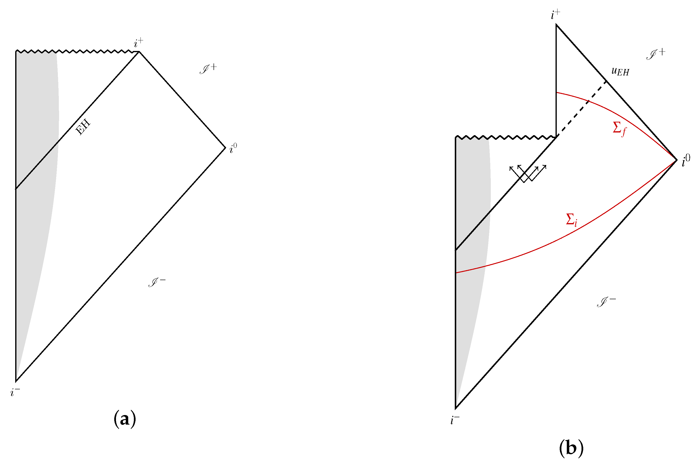
Figure 2.
(a) Part of space–time in which the semi-classical approximation holds. The shaded region depicts an infalling massless scalar field that would give rise to a singularity in classical GR. But loop quantum gravity (LQG) quantum geometry effects intervene to prevent the formation of this singularity. This quantum geometry region and its future are excised (dashed line with scissors). A trapping dynamical horizon (TDH) develops which is space-like with increasing area (in the outward direction) during the collapse, and time-like with decreasing area (in the future direction) during evaporation. Null rays from the contracting part of the TDH go out to meet . Hawking radiation starts in earnest at . The dashed line with scissors that includes the last ray represents the future boundary of the semi-classical region. Evolution from the initial Cauchy surface to generic Cauchy surfaces that lie entirely in the semi-classical region is unitary. However, evolution from to the portion of that lies within the semi-classical region is not. (b) Proposed quantum extension of the space–time. The classical singularity is replaced by a transition surface , to the past of which we have a trapped region, bounded in the past by a trapping dynamical horizon T-DH, and to the future of which we have an anti-trapped region bounded by an anti-trapping dynamical horizon (AT-DH). Cauchy surfaces develop astronomically long necks already in the semi-classical region and the long necks persist also in the quantum region. Partner modes that fall in the trapped region get stretched enormously and are slowly released to the future of the quantum region. Thus, ‘most of the purification’ occurs to the future of the transition surface . The dark (red) blob at the right end of is a genuinely quantum region discussed in Section 2.3 and Section 2.4.

Figure 3.
(a) Classical collapse of a narrow pulse of a massless scalar field, incident from . Note that during the collapse a dynamical horizon (DH) is formed. It is space-like and grows in area as the collapse continues and smoothly joins on to the (null) event horizon (EH) in the distant future. (b) Artist’s depiction of a semi-classical Callen–Giddings–Harvey–Strominger (CGHS) black hole that was analyzed in detail in [33,34]. A Delta-distribution pulse of a scalar field from would lead to a black hole in the classical theory. In the semi-classical theory, the singularity is weakened (the metric is but not ) but persists. The dynamical horizon becomes time-like, shrinks in its ‘area’ due to emission of quantum radiation, terminates and meets the singularity. The dynamical horizon together with the last ray from its endpoint to constitutes the future boundary of the semi-classical space–time.
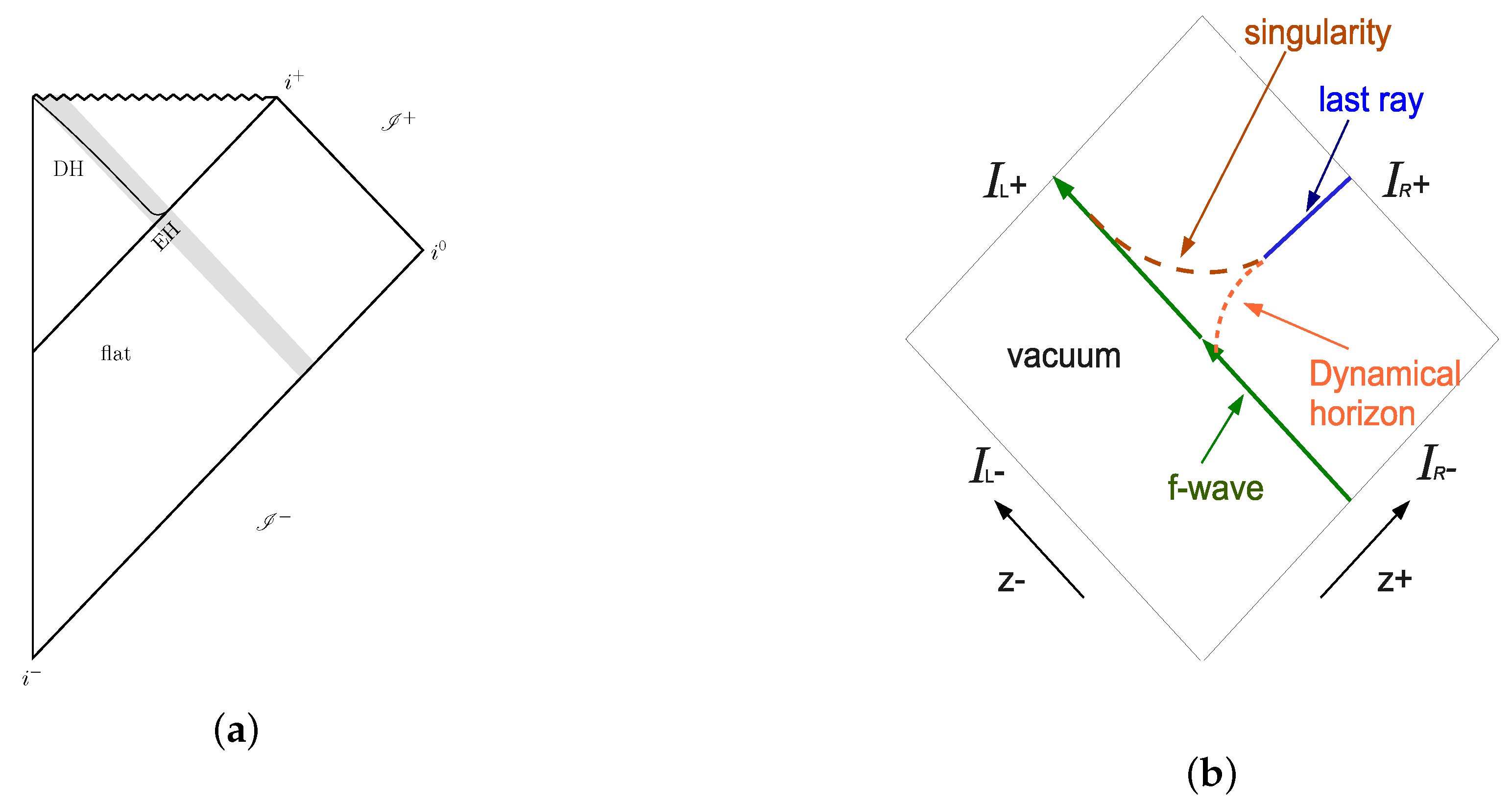
Figure 4.
(a) LQG extension of the Schwarzschild-interior. In classical GR we only have the lower triangular region that is bounded below by the trapping event horizon T-EH and ends with a future space-like singularity at . Quantum geometry effects of LQG resolve this singularity and replace it with a transition surface, labeled , to the future of which we have an anti-trapped region with a future boundary that constitutes an anti-trapping event horizon AT-EH. Quantum geometry effects are important only in a neighborhood of , shown by a shaded (pink) region. (b) LQG extension of the Kruskal space–time [18,19]. Quantum geometry effects resolve both black hole and white hole singularities and the quantum corrected LQG space–time extends indefinitely. The central diamond corresponds to panel (a).The dashed (blue) arrows depict integral curves of the Killing vector. Just as in only a part of the full Kruskal space–time is physically relevant for gravitational collapse in classical GR, only a portion of this infinite extension is relevant for the black hole evaporation process (see Figure 2b).

© 2020 by the author. Licensee MDPI, Basel, Switzerland. This article is an open access article distributed under the terms and conditions of the Creative Commons Attribution (CC BY) license (http://creativecommons.org/licenses/by/4.0/).
Share and Cite
MDPI and ACS Style
Ashtekar, A. Black Hole Evaporation: A Perspective from Loop Quantum Gravity. Universe 2020, 6, 21. https://doi.org/10.3390/universe6020021
AMA Style
Ashtekar A. Black Hole Evaporation: A Perspective from Loop Quantum Gravity. Universe. 2020; 6(2):21. https://doi.org/10.3390/universe6020021
Chicago/Turabian StyleAshtekar, Abhay. 2020. "Black Hole Evaporation: A Perspective from Loop Quantum Gravity" Universe 6, no. 2: 21. https://doi.org/10.3390/universe6020021
Note that from the first issue of 2016, this journal uses article numbers instead of page numbers. See further details here.