A Continuation Procedure for the Quasi-Static Analysis of Materially and Geometrically Nonlinear Structural Problems


Dipartimento di Scienze e Tecnologie Aerospaziali, Politecnico di Milano, Via La Masa 34, 20156 Milano, Italy
*
Author to whom correspondence should be addressed.
Math. Comput. Appl. 2019, 24(4), 94; https://doi.org/10.3390/mca24040094
Submission received: 14 October 2019
/
Revised: 29 October 2019
/
Accepted: 30 October 2019
/
Published: 2 November 2019
(This article belongs to the Special Issue Mesh-Free and Finite Element-Based Methods for Structural Mechanics Applications)
Abstract
:Discussed is the implementation of a continuation technique for the analysis of nonlinear structural problems, which is capable of accounting for geometric and dissipative requirements. The strategy can be applied for solving quasi-static problems, where nonlinearities can be due to geometric or material response. The main advantage of the proposed approach relies in its robustness, which can be exploited for tracing the equilibrium paths for problems characterized by complex responses involving the onset and propagation of cracks. A set of examples is presented and discussed. For problems involving combined material and geometric nonlinearties, the results illustrate the advantages of the proposed hybrid continuation technique in terms of efficiency and robustness. Specifically, less iterations are usually required with respect to similar procedures based on purely geometric constraints. Furthermore, bifurcation plots can be easily traced, furnishing the analyst a powerful tool for investigating the nonlinear response of the structure at hand.
1. Introduction
Nonlinear analyses are commonly performed during the design phases of advanced, modern constructions. An example can be found in the design process of lightweight aerospace structures, where the capability of accurately predicting the behaviour in the post-buckling range is a task of paramount importance. The problem can often be studied by considering just nonlinearties of geometrical nature, where analytical and semi-analytical approaches can be successfully employed [1,2,3,4,5]. However, a proper assessment of damage tolerance demands for numerical simulations capable of predicting also the propagation of cracks, thus including nonlinear effects related to the material response. Meaningful examples illustrating the relevance of nonlinear phenomena in structural problems can be found, e.g., in the works of Refs. [6,7], while qualitative aspects on branching of cracks are reported in Ref. [8]. Due to the inherent complexity of responses involving both geometrical and material nonlinearities, the finite element approach is often the most straightforward one for performing the analysis. In this context, many numerical techniques were developed in the years for handling the peculiar aspects that characterize the response of structures in the nonlinear field. Arc-length strategies have been widely used for solving problems characterized by the presence of limit points. The presence of the load parameter as additional unknown of the problem allows the load to be increased or decreased throughout the iterative process. Pioneering work in this field is due to Riks [9] and Wemper [10]. Noteworthy are the successive efforts to develop the updated normal path method by Ramm and the spherical arc-length by Crisfield [11]. Despite the efficiency in capturing the elastic response of the structure, classical arc-length approaches can be inadequate in the presence of delamination phenomena, as the constraint equation is based on global quantities, while the failure process tends to involve few degrees of freedom. To overcome these limitations, different strategies were proposed based on the modification of the constraint equation to consider the local nodes involved in the delamination process [12,13,14] or by enriching the constraint equation with information regarding the energy dissipated during the process [15,16,17]. An example is found in Ref. [18], where path following techniques were discussed in the framework of Embedded Finite Element Method (E-FEM).
Another class of numerical solution techniques refers to the so-called continuation approach. These path-following techniques were originally introduced by Davidenko [19,20] in the early fifties. They rely on the idea of transforming a nonlinear system of equations into a differential one. The system is parametrized with respect to a solution parameter, and is solved as an initial value problem [21,22,23]. The application of continuation methods to nonlinear structural analyses offers several interesting features. It allows to trace the primary equilibrium path of the structure, also in presence of snaps [24], to detect and compute the critical points [24,25,26] and to trace the bifurcation branches [27,28]. As a result, continuation methods enable to trace the complete bifurcation diagram of the structure, which is of particular interest for gathering deeper insight into the behavior of the structure.
While a consistent number of examples concerning the use of continuation methods for the nonlinear analysis of elastic structures are available in the literature, relatively few applications can be found for handling problems characterized by the presence of crack propagation phenomena. To the best of the authors’ knowledge, no continuation methods were specifically developed for problems involving strain-softening responses.
In this article a novel continuation approach is proposed, offering the capability of handling structural responses characterized by geometrically and materially nonlinear problems. The continuation is performed referring to a modified version of the the Riks’ method [24] in conjunction with a constraint regarding the dissipated energy [15,16]. The approach tries to combine the efficiency of geometric-based procedures in the elastic field, with that of the dissipative ones in the presence of damage. The resulting approach can accurately trace the equilibrium paths and shows excellent robustness on bifurcation branches dominated by dissipative phenomena.
The performance of the approach is demonstrated by means of five numerical examples. The first two ones illustrate the ability of the methods to compute the bifurcation diagram of simple elastic problems. Then, test cases characterized by mixed geometric-material nonlinearities are assessed. Finally, the application of the methods as quasi-static solution strategies is demonstrated in a challenging example dominated by material nonlinearities.
The paper is organized as follows. Introductory aspects on continuation methods are presented in Section 2, where the formulation of the nonlinear finite element approximation is briefly presented. The detection of critical points is discussed in Section 3 by introducing algorithmic aspects for classifying bifurcations and limit points, while the technique for implementing branch-switching is the subject of Section 4. Geometric and dissipative constraint equations are introduced in Section 5, and an overview of the method is provided in Section 6. The application of the method to a set of nonlinear problems is illustrated in Section 7, where test cases involving geometrically and materially nonlinear responses are presented.
2. Preliminaries
Continuation methods are a class of numerical techniques for computing the approximate solution of a system of parametrized nonlinear equations [19,20]. Denoting with the quantity adopted for the parametrization, the procedure consists in constructing an approximation of for a sequence of parameter values in the interval of definition of the parameter itself.
Within the context of the finite element approach, the nonlinear equilibrium equations of a structure can be represented, in their general form, as:
where defines the vector of the internal forces, and provides the shape of the external forces. Nodal displacements are denoted as , while is the load parameter.
The system of Equation (1) can be seen in terms of continuation techniques after noticing that the set of equations defines implicitly a curve of solution points that can be continuously parametrized by means of the parameter . Starting from an initial equilibrium solution condition defined by —which, in turn, corresponds to an initial value of the parameter —the continuation problem consists in calculating the locus of solutions given by the branch . The process is terminated when a target point is reached.
The choice of the parametrization is a focal aspect in the development of a continuation technique. This choice is, in general, not unique and, according to its definition, different methods can be obtained. One possibility is given by the adoption of the load factor , leading to a force-control approach. Another choice consists in considering the displacements of a subset of nodes, which leads to a displacement-based control. These two kinds of parametrization are inadequate for handling turning points, where the surfaces and are tangent to the equilibrium path, and no intersections can be found. On the contrary, a more suitable approach consists in adopting a parametrization that is always nearly orthogonal to the equilibrium path, so that an intersection between the surface and the path is always ensured. This is the case of a parametrization based on the arc-length of the curve s [24]. By introducing a parametrization based on s, the load factor becomes an additional unknown and a scalar constraint equation must be added to Equation (1). The augmented system is then obtained as:
where is the general expression of the additional constraint equation.
Starting from the initial solution , the equilibrium path can be regarded as the solution of the initial value problem obtained by differentiating the augmented system in Equation (2) with respect to s:
where denotes the derivative with respect to the path parameter s.
The solution of Equation (3) can be achieved by using predictor-corrector techniques: the differential problem is initially integrated coarsely, then an iterative method is used as a stabilizer for solving locally .
It is worth observing that predictor-corrector continuation methods are considerably different if compared to the predictor-corrector techniques for the numerical integration of initial value problems. In fact, despite the similarity between the two strategies, the corrector process in the continuation methods thrives on the powerful contractive properties of the solution set for iterative methods such as Newton’s method [21]. This property is not valid for the solution curves of general initial value problems, where the corrector process converges, in the limit, to an approximating point, whose quality depends on the size of the step.
One can observe that the system of Equation (3) involves the presence of derivatives with respect to the parameter s, which is one of the main differences between arc-length and continuation methods. This is an essential feature of continuation methods and allows to easily detect critical points along the equilibrium path and to trace bifurcation branches. The main drawback is given by the need for solving a linear system for computing the derivatives, and to perform an eigenvalue decomposition for detecting critical points.
With this regard, the development of a continuation algorithm capable of tracing the complete bifurcation diagram relies on the definition of:
- a method for detecting and computing critical points, and capable of distinguishing between limit and bifurcation points
- a method for moving from the primary path to a bifurcational branch
- a strategy to follow the equilibrium path along the solution branches
Different continuation methods can be realized by referring to different parametrizations and constraint equations. The performance of the method can be modified by adopting different strategies to perform the prediction or the correction. In addition, a consistent number of procedures can be adopted to perform branch-switching or detect critical points. As result, it is possible to create a wide range of methods characterized by different performance.
In the implementation proposed here, critical points are detected looking at the positive eigenvalues of the stiffness matrix, while their classification is based on the analysis of the stiffness parameter; the eigenvector injection method is adopted for switching from the primary to the bifurcational path, while a novel energy-based path-following technique is proposed for performing the continuation.
3. Critical Points
In this section, the procedure for detecting and approximating the critical points is described. Critical points are equilibrium points corresponding to the singularity of the tangent stiffness matrix . According to the theory of stability of conservative systems, the stability of an equilibrium configuration is ensured by the positive definiteness of the quadratic form , defined as:
where is the tangent stiffness matrix. The transition state between a stable and an unstable equilibrium configuration is characterized by the appearance of a singularity in the matrix . It follows that critical points define the limits of stability of the equilibrium path. The k-th critical point can be defined by means of the following generalized eigenvalue problem:
where and are the k-th eigenvalue and eigenvector of the stiffness matrix, respectively, whereas is the identity matrix.
The eigenvalues are supposed to be arranged according to the sequence
where N is the dimension of the stiffness matrix. When the critical state is reached, one or more eigenvalues in the sequence of Equation (6) are zero.
Critical points can be divided into limit and bifurcation points. In particular the following two conditions are considered:
The first condition of Equation (7) states that the load does not vary with respect to the path parameter in the neighborhood of a limit point. This also means that limit points are equilibrium configurations associated with a local maximum or minimum of the applied load. In most cases, limit points separate stable and unstable equilibrium paths, although this is not a rule. The presence of a limit point is commonly associated with snap-through phenomena, causing sudden snaps to a stable configuration and not adjacent to the original one. In the neighborhood of limit points there exists one unique branch, thus no further equilibrium branches need to be traced.
On the contrary, multiple equilibrium configurations exist in the neighbourhood of a bifurcation point, each of these solutions belonging to a different equilibrium branch and characterized by a different tangent. During the solution process, it is then necessary to distinguish between limit and bifurcation points to establish whether the continuation should be carried out along the emanating branches or not. For this purpose, a procedure based on the evaluation of the stiffness parameter is adopted.
3.1. Stiffness Parameter
The stiffness parameter is a scalar quantity defined as [26]:
where the subscript 0 defines the initial state.
The value of provides a relative measure of the incremental stiffness along the direction in which the solution is moving. During the incremental solution process, this parameter is computed through substitution of the increments into the derivatives, leading to the incremental expression:
where and are the increments computed in the first load step, and and are the total increments computed at the current load step. As seen from Equation (9), the initial value of is equal to one. Whenever the structure loses stiffness with respect to the initial value, viz. and , the parameter becomes smaller than one. On the other hand, if the structure undergoes a stiffening response, i.e., and , is greater than the unity. Furthermore, the stiffness parameter is positive on stable equilibrium branches and negative on unstable branches. As a matter of fact, turns out to be negative for unstable branches because, in such cases, the increment of the load parameter is negative.
An important feature of the stiffness parameter is that, in correspondence of the limit points, it satisfies the condition:
as implicit in the definition of limit point itself. On the other hand, the relative stiffness is different from zero in the presence of a bifurcation point and, after crossing the point, the sign of does not change.
It is worth observing that the condition of Equation (10) is hardly met during the numerical solution of the problem, as the solution is computed for a discrete set of points only. For this reason, the detection of the limit point is performed referring to a numerical approach, described in the next section, for checking the condition given by Equation (10).
3.2. Detection and Classification
Among the various strategies for the computation of critical points [23,25], the approach proposed here is based on the analysis of the sign of the eigenvalues of the tangent stiffness matrix. This approach is simple and robust, and is associated with a relatively small computational effort. It is preliminarly assumed that the eigenvalues of are well separated, which implies that multiple or clustered bifurcations cannot be handled.
The tangent stiffness matrix of a structure, evaluated in its initial, undeformed state, is a positive definite quantity. When a critical point is reached, one eigenvalue, at least, becomes null and, just after crossing the point, the eigenvalue becomes negative. Based on this consideration, it is straightforward to implement the condition:
The critical points subsequent to the first one are captured by monitoring the sign of the lowest positive eigenvalue. In particular, the following condition is employed:
where is the number of positive eigenvalues of the tangent stiffness matrix .
This strategy is particularly simple as the counting of the positive eigenvalues of is just needed.
Once a critical point is detected, the classification between limit and bifurcation points relies upon the valuation of the stiffness parameter (see Equation (10) as outlined in the pseudo-code reported in Algorithm 1.
| Algorithm 1 Classification of critical points. |
|
Note, and are the values of the path parameter s just before and just after the critical point, respectively. The criterion summarized in Algorithm 1 is based on the fact that the stiffness parameter undergoes a change of sign whenever a limit point is crossed. Hence, the critical point is a limit point if a change of sign is detected in , otherwise it is a bifurcation point.
3.3. Approximation
Once critical points are identified and classified, an approximation of the critical state is needed. In continuation methods, bifurcation points are used as initial solutions for tracing bifurcation branches. It follows that the quality of the prediction affects the convergence of the solution along the bifurcation branches. An accurate prediction is then sought. On the other hand, the requirements on the accuracy of the limit point predictions are less strict, as no equilibrium branches emanate from them.
Based on these observations, limit points are determined by means of a linear approximation seeking for the zero of . Given the quantities , , the linear approximation reads:
where and are the values of the path parameter in the converged equilibrium points before and after the critical point, respectively, and:
Setting in Equation (13), and denoting with an asterisk the critical state, the critical load is obtained as:
while the deformed configuration is obtained after substituting Equation (15) into the second of Equation (13), and is obtained as:
This strategy is fast and tends to guarantee satisfactory precision for obtaining an estimate of the limit points.
Regarding the approximation of the bifurcation points, an iterative procedure is implemented to achieve improved accuracy. It is based on the polynomial approximation of the critical point , and seeks the zero of . In turn, the polynomial approximation is obtained through a Taylor expansion of as:
where corresponds to the value of the path parameter at the converged equilibrium solution before the critical point.
A first estimate of the critical state , relative to the point , is given by:
where the vector of the unknowns and its derivative are defined as:
and:
and:
Improved robustness can be achieved by modifying Equation (18) as:
where is a scale factor, chosen while keeping in mind that small values are associated with high accuracy, but high costs, while the opposite holds for high values of . In the present study, a proper tradeoff between quality and computational costs was found by taking equal to 0.1.
A new value of , corresponding to the point , can be computed and, according to Equations (18) and (20), a new estimate of and is also available. The procedure is repeated until convergence is met according to the criterion:
where is the step length adopted to start the analysis, where is the tolerance defined by the user. Based on an extensive set of preliminary investigations, a value of is set by default in the algorithms proposed in this work. To prevent excessively long loops, the criterion of Equation (23) is accompanied by a check on the maximum number of iterations.
4. Branch-Switching Method
After detecting the critical points, a numerical strategy is needed to compute the initial solution, which is then used to start the continuation procedure along the bifurcation branches. An extensive review of branch-switching methods is available in [25]. In the present method, the eigenvector injection method is adopted. It relies on the idea of perturbing the configuration at the critical state by using the eigenvector associated with the eigenvalue [27].
The perturbation is introduced according to:
where is a scale factor defined as:
and is a scalar variable prescribed by the user and referred to as buckling mode scale factor, while the sign of determines the side of the bifurcation branch to be traced.
The initial solution is completed by:
The tangent vector in is approximated as:
After computing the initial solution, it is possible to start the continuation process, and the equilibrium points along the branch are so identified.
It is highlighted that a proper choice of is needed for guaranteeing convergence on the desired branch. If this value is too small, the eigenvector injection method is likely to diverge, whereas a too large value may determine a perturbation size incapable of deviating the solution on the bifurcation branch, and the continuation process is likely to converge on the primary path again [27].
Usually, suitable values of are in the range between 10 and 100. However, no general rules exist for properly selecting the value of , and a trial and error strategy is, generally, the only viable solution.
To deal with this problem, it is necessary that the branch-switching algorithm allows the restart of the analysis of the bifurcation branch with a different value of .
5. Path-Following Continuation Technique
In most cases, continuation techniques are developed by adopting a geometric constraint in Equation (2), an example of which is given by the Riks continuation technique [24]. This kind of constraint is well-suited for those problems dominated by nonlinearities of geometric type. On the contrary, the adoption of a geometric constraint can be source of convergence difficulties whenever the nonlinearities are mainly due to the material response that would lead to localized failure [16]. For instance, this is the case of delamination phenomena, where the strain field is localized in the surroundings of the crack tip. It follows that geometric constraints based on global quantities can be inadequate to capture the deformation process.
Starting from a recent arc-length technique proposed by the authors [17], the continuation technique proposed here tries to overcome the above mentioned difficulties by adopting a modified version of the Riks technique in conjunction with an approach based on the evaluation of the dissipated energy, as outlined in the next sections.
5.1. Modified Riks Method
The modified Riks continuation method is a modified version of the technique described in [24] and relies on a constraint equation involving the displacement vector and its derivative .
As opposed to original implementation proposed by Riks, the equation is adopted here in a modified form, where the contribution due to the load parameter is prevented from entering the equation. In particular, the constraint equation is formulated as:
where denotes an equilibrium point on the path, while is the value of the arc-length at this point; the terms defines an arbitrary point on the surface defined by the constraint equation.
An extensive set of preliminary analyses revealed that Equation (29) offers the main advantage of preventing the doubling back of the solution, a problem often encountered when adopting the classical Riks formulation.
The continuation procedure is performed referring to a predictor-corrector technique, where the increments and are decomposed as:
where and are the total increments at the current step, and are the iterative increments at the last iteration j, and and are the iterative increments referred to the current ()iteration.
The predictor solution is computed according to:
The corrector phase is performed referring to the Newton’s method, which is applied to solve the augmented system of Equation (2) using Equation (29) as constraint, so:
where is the residual at the end of the j-th iteration, defined as:
Substituting Equation (30) in Equation (32), the iterative increments and are obtained as:
having assumed that , and
It is worth noting that Equation (34)b resembles the expression of of the Riks arc-length method [24]. However, the two equations differ in the term of Equation (34)b, viz., the derivative of the displacement vector in the last converged equilibrium point, which is replaced by the displacement increment of the predictor step in the Riks formulation.
To gather insight into the constraint equation developed here, it is possible to compare Equations (34)b and (29), and re-write the constraint as:
The expression of Equation (36) defines a hyperplane in the subspace of displacements, which is normal to the vector . In addition, Equation (36) can be thought as the projection of the Riks constraint equation onto the subspace of displacements.
After reaching convergence, the tangent vector is computed by solving the linear system obtained from the differentiation of Equation (32) with respect to s. The linear system is derived as:
The vector defines the direction of the tangent vector, but not its orientation [22]. To this aim the scalar is introduced as:
On the basis of the sign assumed by , the orientation is defined by reversing when . This criterion imposes that the tangent vector points towards the direction that forms an angle smaller than with respect to the last computed displacement increment .
5.2. Dissipated Energy Method
The adoption of a purely geometric constraint equation can be inadequate for analyzing those probelms characterized by material nonlinearities, especially in the presence of strain-softening responses. To overcome these difficulties, a second constraint, to be used in conjunction with the previous geometric one, is introduced.
The method makes use of the energy release rate G. In the context of the finite element approximation, it is obtained as [16]:
where the symbol denotes differentation with respect to time.
Applying a forward Euler approximation of Equation (39), the expression of the energy dissipated in the current step, , is obtained as:
where is the total dissipated energy and the amount of energy dissipated up to the last converged equilibrium condition. From inspection of Equation (40), a constraint equation for the continuation method can be derived as:
where the parametrization is now performed with respect to the parameter , i.e., the dissipated energy, instead of the arc-length s. More specifically, the constraint specified by Equation (41) imposes that the energy dissipated in the current load step is equal to the amount .
As done for the modified Riks continuation, a predictor-corrector method is employed for solving the governing equations. However, derivatives are now taken with respect to the parameter . The predictor step is then:
while the corrector phase is based upon the Newton solution of Equation (2) together with Equation (41), leading to the linearized system:
By substituting Equation (30) into Equation (43), the system can be represented in matrix form as:
where:
and:
The iterative increments and are computed from Equation (44) applying the Sherman–Morrison formula [16]):
where the terms and are the solutions of the following linear systems:
After reaching convergence, the tangent vector is computed through the solution of the linear system obtained by taking the derivative with respect to of Equation (43):
5.3. Switching from Geometric to Dissipation-Based Constraints
Aiming at combining the advantages (and ranges of employment) of the techniques previously outlined, a single continuation approach is developed based on the geometric and dissipation strategies. As a matter of fact, the strategy based on the dissipated energy cannot be adopted in the context of purely elastic conditions, as it would fail to converge to the equilibrium solution. Similarly, convergence issues could arise when the modified Riks approach is adopted in the presence of damage phenomena. For this reason, the two approaches are combined referring to amount of energy dissipated. In particular, two threshold values are defined, namely and .
The analysis is started by adopting the modified Riks continuation method to trace the first load steps, which are always elastic, provided their size is chosen to be sufficiently small. When the energy dissipated in the current step exceeds , the dissipative continuation technique is activated. Then, as soon as the energy dissipated during the current step falls below , the solution strategy is switched back to the modified Riks continuation. In absence of specific motivations, the two thresholds can be generally be taken equal each other. The approach is summarized in Algorithm 2.
| Algorithm 2 Switch between two continuation techniques. |
|
It is remarked that the adoption of the two mentioned strategies determines the presence of a double parametrization, as the modified Riks continuation method is parametrized with respect to the arc-length s, and the dissipated energy constraint equation relies on the parameter . This peculiarity may be source of difficulties whenever a critical point is detected between two equilibrium points computed by means of different strategies (e.g., one adopting the modified Riks continuation method and the other adopting the dissipative procedure). This aspect has to be carefully monitored during the solution process, and possible critical points so obtained should be recomputed.
6. Implementation
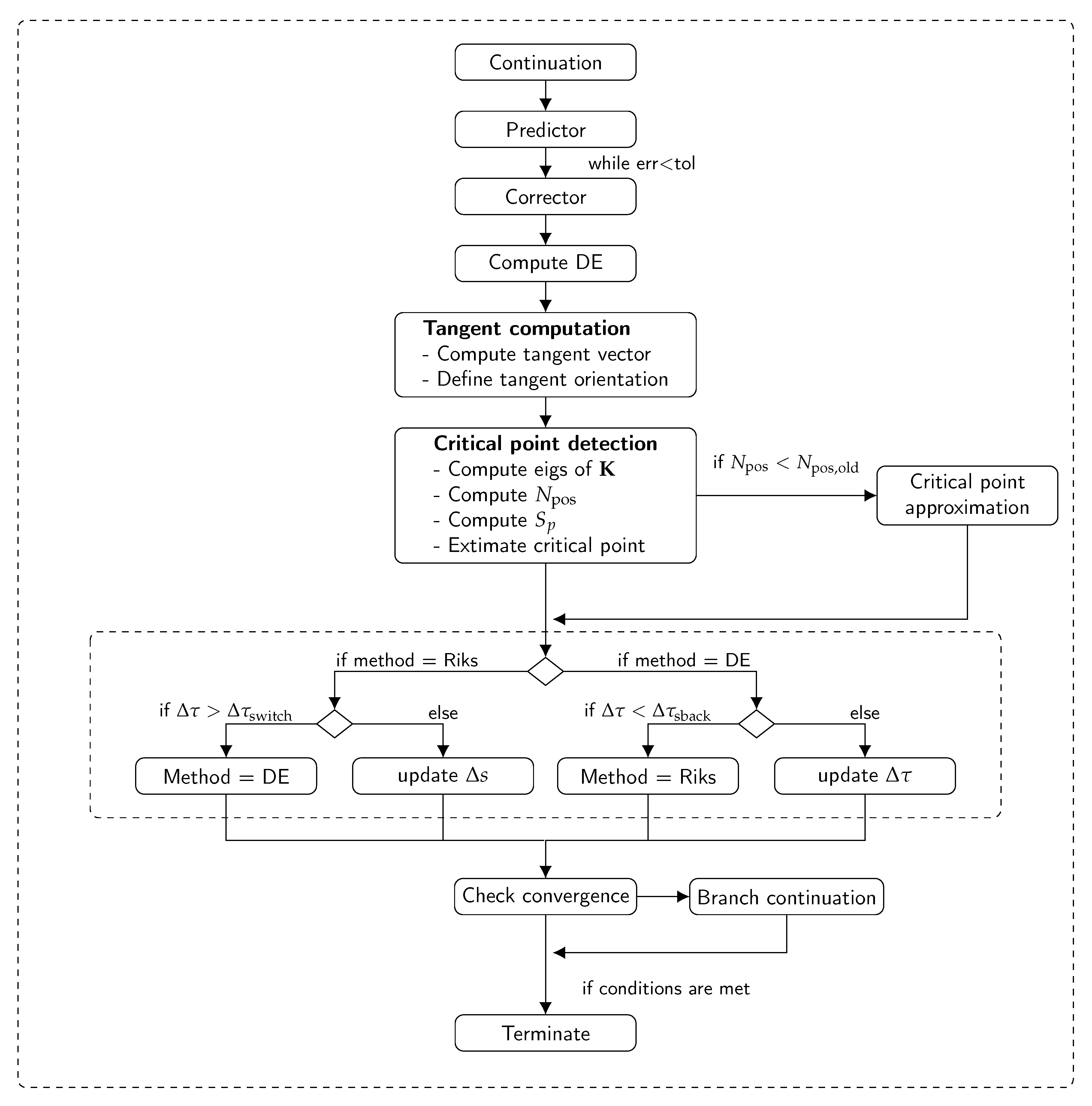
To clarify the various steps involved in the solution process, an overview of the method is provided in the flowchart of Figure 1. The relevant equations adopted at each steps are reported by observing that they vary according to the continuation strategy currently active – this can be either the modified Riks or the dissipation-based method.
At the beginning of the procedure, the modified Riks method is set by default, so all the equations reported henceforth are those relative to the Riks approach during the first loop. The initial predictor step is performed on the basis of Equation (31) or (31), while Newton-Raphson iterations are repeated during the corrector phase referring to Equation (37) or (43). The procedure is arrested when the error is below the threshold defined by the tolerance. The successive step consists in the evaluation of the dissipated energy, which is used subsequently to define the continuation algorithm. The evaluation of the tangent vector requires the solution of the linear systems according to Equation (37) or (49), while the parameter of Equation (38) is adopted for defining the orientation.
The successive phase consists in detecting the critical points, which is performed by evaluating the eigenvalues of the stiffness matrix . Depending on the number of positive eigenvectors and the value of the stiffness parameter, it can be established whether a critical point is obtained, and its nature, i.e., bifurcation or limit. After detecting a critical point, the approximation procedure is activated following the procedure outlined in Section 3.3.
The method to be used in the subsequent step is defined by comparing the dissipated energy with the threshold values defined by the user. In the presence of dissipation phenomena, the method is set as DE, otherwise the Riks continuation is maintained. Note that the switch between the two strategies is controlled by the algorithm outlined in Algorithm 2.
The step length is finally updated following the approach presented in Ref. [17], and convergence is finally checked. Whenever one or more bifurcation points are detected throughout the iteration process, the continuation along the secondary equilibrium path is performed.
7. Results
In this section, the continuation strategy is applied to the analysis of problems involving both geometric or material nonlinearities. These kind of nonlinearities can be present independently or in combination. All the simulations are performed using the open source finite element code PyFem [29], that was used as underlying framework for implementing the numerical procedure. The elements used for the analyses are nonlinear four-node, plane-strain continuum elements. To model delamination phenomena, the cohesive element proposed by Camanho et al. [30] was implemented in PyFem. Mesh sizes were defined on the basis of preliminary convergence studies. In those analyses involving the use of cohesive elements, the mesh size was chosen to guarantee a proper description of the process zone, referring to the length defined by [31,32]:
where is a scalar nondimensional parameter, here taken as 0.884, E denotes the Young’s modulus, is the fracture toughness in mode I, and N is the interfacial strength.
It is noted that the ability of the method to converge to the correct solution and to successfully trace the bifurcation diagrams is strongly affected by the choice of the parameter . To this aim, preliminary tests were carried out to properly choose the value of the parameter.
The section of results is organized as follows. Two preliminary test cases, an axially compressed column and a simple one-degree-of-freedom (one-DOF) problem, are discussed in Section 7.1 and Section 7.2 to illustrate the application of the method to geometrically nonlinear problems. The application of the continuation approach is then presented for two problems, a beam and an arch embedding initial cracks, in Section 7.3 and Section 7.4, where materially nonlinear responses are of concern. Bifurcation plots are presented for these two cases, and the robustness of the approach is illustrated against an alternative formulation based on a purely geometric constraint equation. Finally, the procedure is presented as a mean for solving quasi-static problems for a relatively complex nonlinear example, a perforated beam loaded in mode I, which is discussed in Section 7.5.
7.1. Subcritical Bifurcation (One-DOF Problem)
This first example deals with the nonlinear response of a simple 1-DOF problem characterized by the presence of a sub-critical bifurcation point. It follows that equilibrium branches emanating from the bifurcation are, in this case, unstable. The structure is composed by a rigid truss and a linear spring, as illustrated in Figure 2. The length l is equal to 10 mm, while the stiffness of the spring is N/mm. An horizontal load of intensity P is applied at the free end of the rigid bar.
The numerical model is obtained by using a linear spring element and truss with a very high stiffness value to simulate the ideal infinite value.
The numerical predictions obtained with the proposed continuation method are compared with the analytical solution of the problem, which is given by:
where is the rotation angle and P the applied load. The results are summarized in Figure 3.
As observed, perfect matching is achieved when comparing the analytical and the numerical solution. The continuation procedure correctly identifies the overall bifurcation plot, and provides an accurate description of the three equilibrium paths emanating from the bifurcation point. Note that the solution process is carried out without activation of the dissipative continuation technique as the response is purely elastic.
7.2. Supercritical Bifurcation (Axially Compressed Column)
The second assessment regards the analysis of a column subjected to a compressive end load. The bifurcation is defined as supercritical as both sides of the bifurcation branch are locally stable equilibrium paths characterized by increasing values of the load factor [23]. A sketch of the structure is provided in Figure 4. The column is fixed at one end and free at the second one, while a concentrated force is applied at the free end. The overall length l is equal to 10 mmand the thickness h is 1 mm. An isotropic homogeneous material of modulus GPa and is assumed. Ten finite elements are used for discretization.
The problem does not involve any kind of dissipative phenomena, so the modified Riks continuation approach is maintained throughout the solution process. The results are compared against those obtained by using the Crisfield arc-length approach, whose implementation in the PyFem code was already assessed in Ref. [17]. It is worth noting that the Crisfield method is not developed for tracing bifuraction diagrams in one single run. For this reason, two distinct nonlinear analyses were performed by assuming initial imperfections with opposite sign and shape equal to the first buckling mode. On the contrary, the continuation method allows to plot the bifuraction diagram in one single run, with no need for introducing initial imperfections.
The results are summarized in Figure 5, where the axial displacement of the bottom-most corner of the column is reported against the axial load.
The close matching with the results obtained using the Crisfield method demonstrates the ability of the continuation method to deal with the solution of equilibrium branches arising from supercritical bifurcation points.
In addition, the quality of the prediction can be noted by inspection of the region in the neighborhood of the bifurcation. As seen from the zoom of the plot, the continuation approach provides a precise description of the equilibrium branches departing from the critical point. In contrast, the Crisfield approach undergoes small oscillations, and convergence to spurious equilibrium configurations is observed in proximity of the bifurcation. Again, it is remarked that no initial imperfections are needed within the context of the continuation approach, so the bifurcation is precisely detected.
7.3. Beam Containing an Initial Crack
Previous test cases are restricted to geometrically nonlinear phenomena, and material nonlinearities are not accounted for. In the example presented here, a beam containing an initial delamination is considered and the propagation of the crack is accounted for by making use of cohesive elements characterized by a bilinear cohesive law. Further details regarding the implementation of these elements in the PyFem code are available in [33]. A sketch of the structure is reported in Figure 6.
The beam’s length and thickness are denoted with l and h, respectively. The central portion of the beam is characterized by the presence of an initial crack, whose length is equal to a. The material is isotropic with modulus GPa and Poisson’s ratio 0.25, and a plane strain constitutive law is assumed.
The structure is hinged at the bottom left vertex, while the translation along the direction normal to the beam axis is constrained at the bottom right end. The load is introduced in the form of a compressive force per unit length of magnitude p.
As seen from Figure 6, the structure is divided into two equal parts with respect to the midline running parallel to the beam axis. The two outer portions are connected by means of two layers of cohesive elements. The fracture toughnesses in mode I and II are taken as 0.5 N/mm, while the interfacial strengths are fixed at 1.0 . The penalty stiffness of the cohesive elements is 5000 .
The centrally located pre-damaged area is simulated by means of cohesive elements with reduced properties, whose aim is to avoid interpenetration between the upper and lower parts of the structure during the deformation process [32].
The finite element model is composed of 200 nonlinear shell elements and 20 cohesive elements. Note, the mesh size is chosen in order to guarantee the presence of 4/5 elements in the process zone, whose size is estimated referring to Equation (50).
In the first part of the procedure, the primary equilibrium path is computed. Starting from the undeformed configuration, the load is progressively increased, and the corresponding equilibrium points are found. During this first phase, the eigenvalues of the stiffness matrix are determined at each step of the iterative process, and the presence of critical points is verified. Whenever a critical point is detected, it is approximated referring to the procedure outlined in Section 3, depending on whether it is a limit or a bifurcation point. As an example, the initial part of the primary path is reported in Figure 7a, just after the detection of the first bifurcation point. The procedure is then switched to the continuation procedure, and the tracing of the equilibrium path restarts from the last equilibrium point available. The complete primary path up to a load of 300 N is presented in Figure 7b together with the four bifurcation points detected.
As reported in Figure 7b, the primary path is characterized by an almost linear behaviour, consisting of a progressive shortening of the beam with no bending deflections. After the first bifurcation point, the primary equilibrium path becomes unstable. However, the absence of initial imperfections and the symmetry of the problem make its computation possible. It is also noted that no damage phenomena are associated with this primary equilibrium configurations.
In the second phase of the solution process, the equilibrium branches departing from the bifurcation points are computed. The branch associated with a positive sign of the first buckling mode is plotted in Figure 8a, while the branch obtained by assuming a negative sign is reported in Figure 8c. The two corresponding deformed shapes are presented in in Figure 8b,d, respectively.
In a similar fashion, the procedure is repeated for all the bifurcations points. The results of Figure 9 illustrate the force-displacement curves and the corresponding deformed shapes during the evaluation of the fourth equilibrium branch.
The curve of Figure 9c corresponds also with the complete bifurcation diagram, comprehensive of all the equilibrium paths departing from the bifurcation points detected.
A summary of the deformed configurations obtained at the end of the loading process along the four equilibrium branches is reported in Figure 10.
From Figure 10 it can be noted that all the deformed shapes but the third one exhibit the typical buckled pattern of pristine beams. In this case, the deformed configurations are characterized by one to three half-waves, and a partial damaging of the cohesive elements is observed due to the shear transfer mechanism between the upper and lower portion of the beam. As result, the fracture is dominated by a mode II mechanism. As observed from Figure 9c, the corresponding load-deflection curves are associated with a slight drop of load just after the bifurcation point, motivated by the contemporary onset of the buckling half-waves and damage mechanism in mode II. Afterwards, no additional load is carried by the structure, and the shortening happens at a constant load level.
A different response is observed for the third equilibrium branch, whose post-buckled pattern is reported in Figure 10c. In this case, the damage mechanism is governed by mode I component, with a clear opening between the upper and lower portions of the structure. The propagation is unstable and sudden, and is responsible for a drastic drop of load, not clearly visible from the complete bifurcation diagram. For clarity purposes, the force-displacement curve is reported in Figure 11 by restricting the plot to the third equilibrium branch, where the collapse induced by the onset of the buckling phenomenon can be fully appreciated.
The unloading phase happens in a steep manner, along a path which is close, but distinct, from loading one. After the drop of load, all the cohesive elements are completely damaged, thus the solution is arrested.
It is interesting to investigate the performance of the method in terms of number of iterations along the equilibrium branches previously considered. The results are summarized in Table 1 with regard to two different solution procedures. In one case, denoted with hybrid, the procedure refers to the combined geometric-dissipative approach summarized in Figure 1; in the other case, denoted with geometric, the dissipative constraint is removed, and the procedure is forced to adopt the purely geometric Riks constraint. As far as the number of iterations is a function of the parameter of Equation (25), a preliminary assessment was performed to obtain the values of —reported in the brackets—guaranteeing the smallest number of iterations.
As summarized in Table 1, the adoption of the dissipative constraint determines an increase of the total number of iterations with respect to the modified Riks case. The increase is motivated by the mainly geometric nature of the post-critical configurations associated with the equilibrium branches 1, 2 and 4. In these cases, the sources of nonlinearity can be mostly attributed to the deflected patterns, as seen from Figure 10, thus the advantages offered by a dissipation based-criterion cannot be fully appreciated. On the contrary, the number of iterations is slightly smaller when the combined dissipative-geometric constraint is adopted for tracing the third equilibrium branch, i.e., the one characterized by the opening of the initial crack. While the comparison in terms of iterations seems to suggest the adoption of a purely geometric constraint, it is important to notice that the quality of the predictions in the two cases is not equal. In particular, the adoption of a geometric constraint tends to determine relatively large increments, and the step size can be hardly controlled. It follows that the equilibrium path is not accurately described. On the other hand, the adoption of a dissipative constraint provides an excellent control of the step size, so enabling to trace the equilibrium branches with improved degree of refinement.
7.4. Fixed-Fixed Arch
An additional example is discussed regarding the configuration illustrated in Figure 12.
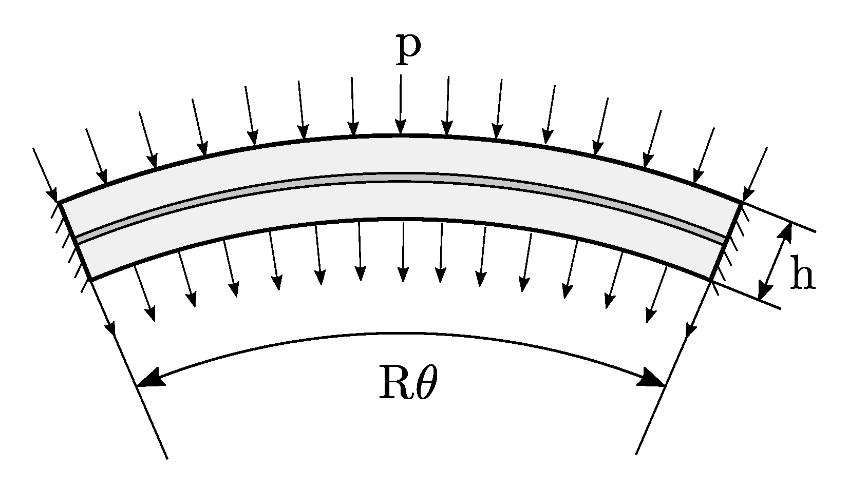
The structure is an arch characterized by a radius R equal to 10 mm, an arc-length angle of radians, and a radius-to-thickness ratio of 100. The material elastic properties are those considered in the previous example. The two ends of the beam are fixed, while a uniformly distributed force per unit length p is applied along the radial direction at the upper and lower surface of the arch, as illustrated in Figure 6. In order to account for material nonlinear responses, a layer of cohesive elements is introduced along the midline of the arch. In this case the fracture toughnesses in mode I and II are 0.5 N/mm, while the interfacial strengths are equal to 15 . The mesh is made of 100 nonlinear shell elements and 50 cohesive elements.
The bifurcation plot is presented in Figure 13 by reporting the nodal displacement of the central upper node versus the nodal force applied at the same node.
In this case, two critical points are detected along the primary path. The first one is a bifurcation point, as seen from the equilibrium path emanating from it. The second one is a limit point, and corresponds to a local maximum of the load carried by the structure. The primary path is now characterized by a nonlinear behaviour, where a progressive reduction of the linear stiffness is observed. No damage phenomena are observed along the major part of this path, as cohesive elements display the initiation of damage mechanisms just in the surroundings of the limit point.
The secondary equilibrium branch is characterized by an unloading phase, associated with a progressive failure of all the cohesive elements in mode II. From the curve of Figure 13, it can be observed the step-wise shape of the secondary equilibrium path, which is related to the failure of the interface elements. In any case, the layer of cohesive elements is distributed along all the overall structure, thus the role played by dissipative phenomena is significant.
To further address the relevance of dissipative phenomena, a comparison is presented between the performances achieved by considering the geometric-dissipative constraint, and those obtained with a run based on the adoption of a purely geometric constraint. The number of increments and iterations to complete the analysis are summarized in Table 2, where the optimal value of the parameter is reported in the brackets.
In this test, the advantages offered by the use of the hybrid constraint are clearer. While the number of increments along the two paths is, by chance, identical, the total number of iterations is much smaller when the energy control is active. The reduction of iterations determines a gain of approximately 15% in terms of computational time. In fact, the post-bifurcational response is dominated by the material nonlinearities, so the control over the dissipated energy is the more efficient approach.
7.5. Perforated Beam
This final example illustrates the use of the continuation approach as a mean for solving a nonlinear problem characterized by a complex response, where nonlinearites are due to geometric and material behaviour. The numerical solution strategy is not used here for tracing the bifurcation plot, but for obtaining the primary equilibrium path, as commonly done when solving a nonlinear quasi-static problem. The problem was analyzed using arc-length hybrid strategies in a previous work form the authors [17].
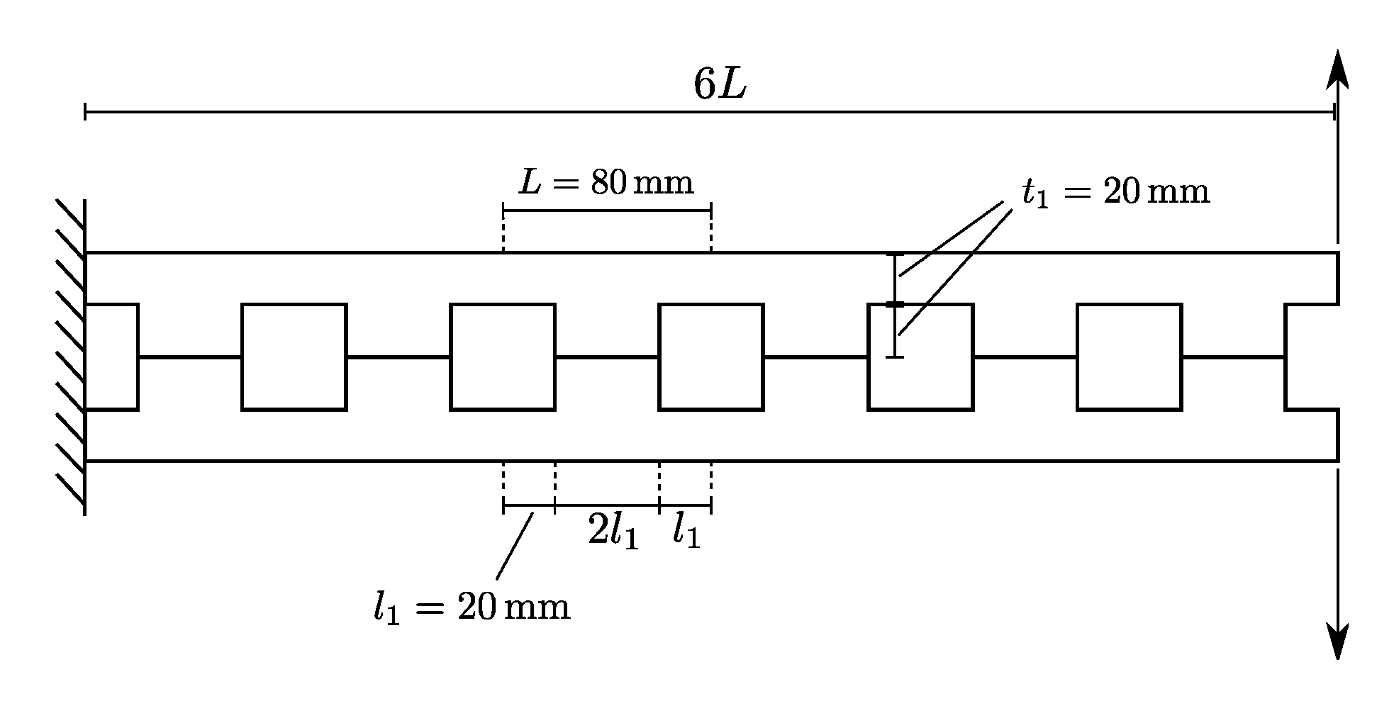
The analysis regards the mode I opening of a cantilever beam characterized by the presence of five equally spaced, square holes. The beam is loaded at the tip by means of two concentrated forces, as indicated in Figure 14, where all the relevant geometric dimensions are reported. An isotropic material is considered, with modulus equal to 1000 MPa and Poisson’s ratio 0.3.
To capture the onset and the propagation of the crack, a layer of cohesive elements is introduced along the horizontal line of symmetry of the structure. The fracture toughnesses in mode I and II are equal to 0.01 N/mm, while the interfacial tensile and shear strength are taken as 1 . A penalty stiffness of 100 is assumed. The resulting finite element model is composed of 288 two-dimensional, plane-strain continuum elements, and 24 cohesive elements.
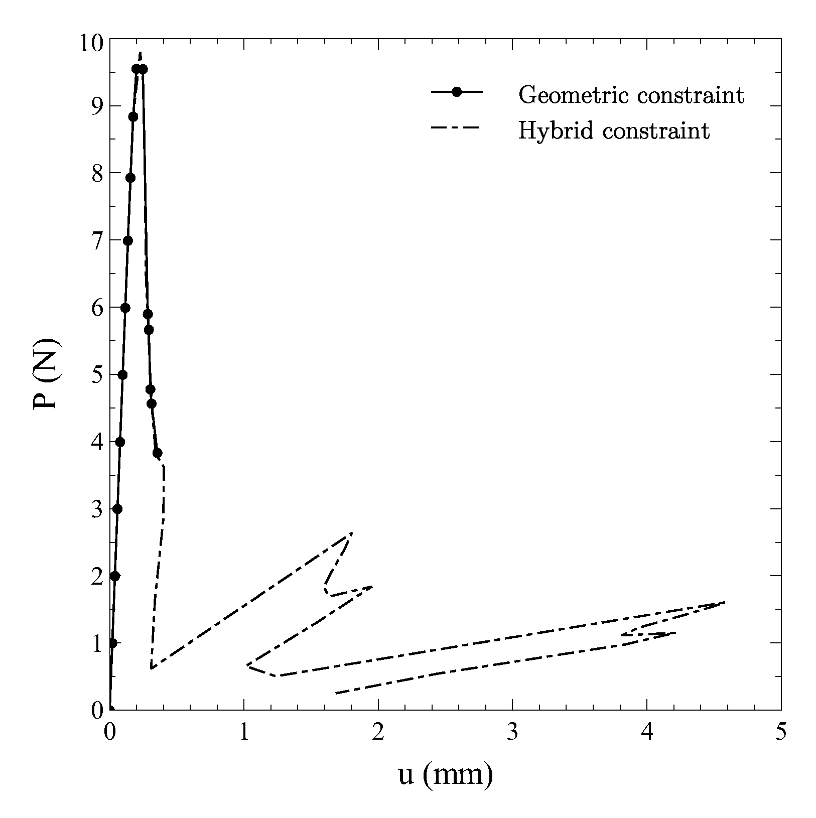
The curves reporting to the vertical displacement of the loaded nodes are plotted against the applied load in Figure 15. The comparison is presented for two different strategies. In one case the continuation method is applied as implemented, thus allowing the automatic switch between geometric and dissipative constraint. In the second case the constraint is forced to be of purely geometric, with the scope of illustrating the advantages due to the hybrid continuation approach presented here.
As seen from the figure, the adoption of a purely geometric constraint leads to a premature failure of the analysis, which terminates along the first descending branch of the curve. On the contrary, the hybrid implementation is capable of capturing the subsequent portions of the equilibrium path. Note that each sudden drop is due to the opening of the holes. After the first peak, a snap-back behaviour can be observed, where a secondary snap characterizing the unloading phase. Indeed, a partial recovery of the load-carrying capability is observed in the post-peak region, followed by another snap-back.
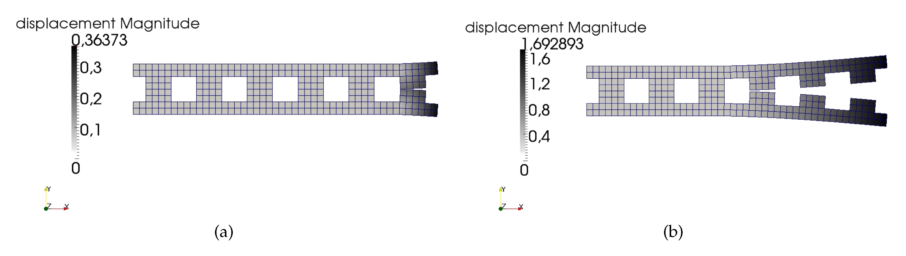
The deformed shapes at the end of the analysis are reported in Figure 16.
While the initiation of the opening of the first crack coincides with the failure of the purely geometric approach (Figure 16a), the improved robustness properties of the hybrid method are clearly visible from Figure 16b.
It is useful to illustrate the comparison between the two strategies in terms of numerical performance of the solution procedure, as done in Table 3.
The results provide a clear picture of what highlighted by inspection of the force-displacement response. In particular, the geometric continuation is capable of obtaining the solution in the initial part of the curve, where 17 increments are performed. At the onset of the first crack, the step length is reduced 3 times, demonstrating the difficulties experienced by the method to obtain the solution. Then, after reaching the complete damaging of two cohesive elements, the analysis is terminated.
On the other hand, the hybrid strategy is capable of reaching the condition characterized by a number of 12 completely damaged cohesive elements. No step length reductions are observed. Clearly, the total time for the analysis and the number of increments are higher.
8. Conclusions
This work discussed the development and implementation of a numerical continuation technique for analyzing structural problems characterized by geometric and material nonlinearities. The continuation strategy can be successfully applied for detecting bifurcation and limit points as well as tracing the equilibrium paths, which is a useful mean for gathering insight into the response of the structure. For instance, the complete post-buckling behaviour can be assessed by performing one single quasi-static analysis, with no needs to introduce initial imperfections in the finite element model.
The effectiveness of the current implementation was checked by means of illustrative examples, where cohesive elements were employed for capturing the onset and propagation of cracks. Main advantage of the approach is the robustness of the numerical solution strategy, which is based upon a hybrid constraint equation that includes both geometric and dissipative considerations. Thus crack propagation phenomena can be accurately predicted, whilst standard geometric-based approaches tend to undergo converge issues. In addition, the method can be used as a technique for solving quasi-static nonlinear problems, when the analysis of secondary equilibrium paths is not of concern. The effectiveness of the approach was illustrated with a test case characterized by the presence of sharp snap-backs, and secondary snap-backs. The analyst can benefit for the adoption of a unique, integrated solution scheme, which can be used for solving the structural boundary value problem, as well as exploring multiple equilibrium paths with improved robustness.
Author Contributions
The two authors equally contributed to the present paper.
Acknowledgments
This study did not receive funds.
Conflicts of Interest
The authors declare no conflict of interest.
References
- Buermann, P.; Rolfes, R.; Tessmer, J.; Schagerl, M. A Semi-Analytical Model for Local Post-Buckling Analysis of Stringer- and Frame-Stiffened Cylindrical Panels. Thin Walled Struct. 2006, 44, 102–114. [Google Scholar] [CrossRef]
- Brubak, L.; Hellesland, J. Semi-analytical Postbuckling and Strength Analysis of Arbitrarily Stiffened Plates in Local and Global Bending. Thin Walled Struct. 2007, 45, 620–633. [Google Scholar] [CrossRef]
- Vescovini, R.; Bisagni, C. Two-step procedure for fast post-buckling analysis of composite stiffened panels. Comput. Struct. 2013, 128, 38–47. [Google Scholar] [CrossRef]
- Barriére, L.; Marguet, S.; Castanié, B.; Cresta, P.; Passieux, J.C. An adaptive model reduction strategy for post-buckling analysis of stiffened structures. Thin Walled Struct. 2013, 73, 81–93. [Google Scholar] [CrossRef] [Green Version]
- Milazzo, A.; Oliveri, V. Post-buckling analysis of cracked multilayered composite plates by pb-2 Rayleigh–Ritz method. Compos. Struct. 2015, 132, 75–86. [Google Scholar] [CrossRef]
- Cricrì, G.; Perrella, M.; Calì, C. Experimental and numerical post-buckling analysis of thin aluminium aeronautical panels under shear load. Strain 2014, 50, 208–222. [Google Scholar] [CrossRef]
- Citarella, R.; Giannella, V.; Lepore, M. DBEM crack propagation for nonlinear fracture problems. Frattura ed Integrità Strutturale 2015, 34, 514–523. [Google Scholar]
- Pook, L. Determination of fatigue crack paths. Int. J. Bifurc. Chaos 1997, 7, 469–475. [Google Scholar] [CrossRef]
- Riks, E. The Application of Newton’s Method to the Problem of Elastic Stability. J. Appl. Mech. 1972, 39, 1060–1065. [Google Scholar] [CrossRef]
- Wempner, G. Discrete approximations related to nonlinear theories of solids. Int. J. Solids Struct. 1971, 7, 1581–1599. [Google Scholar] [CrossRef]
- Crisfield, M. A fast incremental/iterative solution procedure that handles “snap-through”. Comput. Struct. 1981, 13, 55–62. [Google Scholar] [CrossRef]
- May, I.; Duan, Y. A local arc-length procedure for strain softening. Comput. Struct. 1997, 64, 297–303. [Google Scholar] [CrossRef]
- Schellekens, J.; Borst, R.D. A non-linear finite element approach for the analysis of mode-I free edge delamination in composites. Int. J. Solids Struct. 1993, 30, 1239–1253. [Google Scholar] [CrossRef] [Green Version]
- Borst, R.D. Computation of post-bifurcation and post-failure behavior of strain-softening solids. Comput. Struct. 1987, 25, 211–224. [Google Scholar] [CrossRef] [Green Version]
- Gutierrez, M. Energy release control for numerical simulations of failure in quasi-brittle solids. Commun. Numer. Methods Eng. 2004, 20, 19–29. [Google Scholar] [CrossRef]
- Verhoosel, C.; Remmers, J.; Gutierrez, M. A dissipation-based arc-length method for robust simulation of brittle and ductile failure. Int. J. Numer. Methods Eng. 2009, 77, 1290–1321. [Google Scholar] [CrossRef]
- Bellora, D.; Vescovini, R. Hybrid geometric-dissipative arc-length methods for the quasi-static analysis of delamination problems. Comput. Struct. 2016, 175, 123–133. [Google Scholar] [CrossRef] [Green Version]
- Rastiello, G.; Riccardi, F.; Richard, B. Discontinuity-scale path-following methods for the embedded discontinuity finite element modeling of failure in solids. Comput. Methods Appl. Mech. Eng. 2019, 349, 431–457. [Google Scholar] [CrossRef] [Green Version]
- Davidenko, D. On a new method of numerical solution of systems of nonlinear equations. Doklady Akademii Nauk SSSR 1953, 4, 601–602. (in Russian). [Google Scholar]
- Davidenko, D. On approximate solution of systems of nonlinear equations. Ukrainian Math. J. 1953, 5, 196–206. (in Russian). [Google Scholar]
- Allgower, E.; Georg, K. Introduction to Numerical Continuation Method; SIAM: Philadelphia, PA, USA, 2003. [Google Scholar]
- Rheinboldt, W. Numerical Analysis of Continuation Methods for Nonlinear Structural Problems. Comput. Struct. 1981, 13, 103–113. [Google Scholar] [CrossRef]
- Seyde, R. Practical Bifurcation and Stability Analysis; Springer: New York, NY, USA, 2009. [Google Scholar]
- Riks, E. An incremental approach to the solution of snapping and buckling problems. Int. J. Solids Struct. 1979, 2, 529–551. [Google Scholar] [CrossRef]
- Shi, J. Computing critical points and secondary paths in nonlinear structural stability analysis by the finite element method. Comput. Struct. 1996, 58, 203–220. [Google Scholar] [CrossRef]
- Bergan, P.; Horrigmoe, G.; Bråkeland, B.; Søreide, T. Solution techniques for non- linear finite element problems. Int. J. Numer. Methods Eng. 1978, 12, 1677–1696. [Google Scholar] [CrossRef]
- Wagner, W.; Wriggers, P. A simple method for the calculation of postcritical branches. Eng. Comput. 1988, 5, 103–109. [Google Scholar] [CrossRef]
- Magnusson, A.; Svensson, I. Numerical treatment of complete load–deflection curves. Int. J. Numer. Methods Eng. 1998, 41, 955–971. [Google Scholar] [CrossRef]
- Borst, R.D.; Crisfield, M.; Remmers, J.; Verhoosel, C. Non-Linear Finite Element Analysis of Solids and Structures; John Wiley & Sons: New York, NY, USA, 2012. [Google Scholar]
- Camanho, P.; Dávila, C.G.; Moura, M.D. Numerical simulation of mixed-mode progressive delamination in composite materials. J. Compos. Mater. 2003, 37, 1415–1424. [Google Scholar] [CrossRef]
- Turon, A.; Dávila, C.; Camanho, P.; Costa, J. An Engineering Solution for Using Coarse Meshes in the Simulation of Delamination with Cohesive Zone Models. Available online: https://ntrs.nasa.gov/search.jsp?R=20050160472 (accessed on 30 October 2019).
- Vescovini, R.; Dávila, C.; Bisagni, C. Failure analysis of composite multi-stringer panels using simplified models. Compos. B Eng. 2013, 45, 939–951. [Google Scholar] [CrossRef]
- Bellora, D. Quasi-Static Solution Procedures for the Finite Element Analysis of Delaminations. Master’s Thesis, Politecnico di Milano, Milano, Italy, 2015. [Google Scholar]
Figure 1.
Flowchart of the continuation procedure.

Figure 2.
Sketch of the truss-spring system.
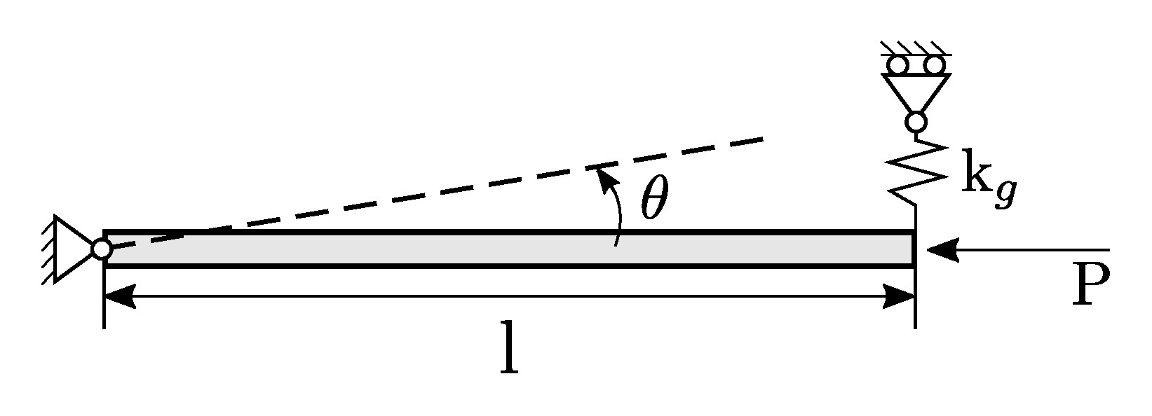
Figure 3.
Bifurcation plot for the spring-truss example.
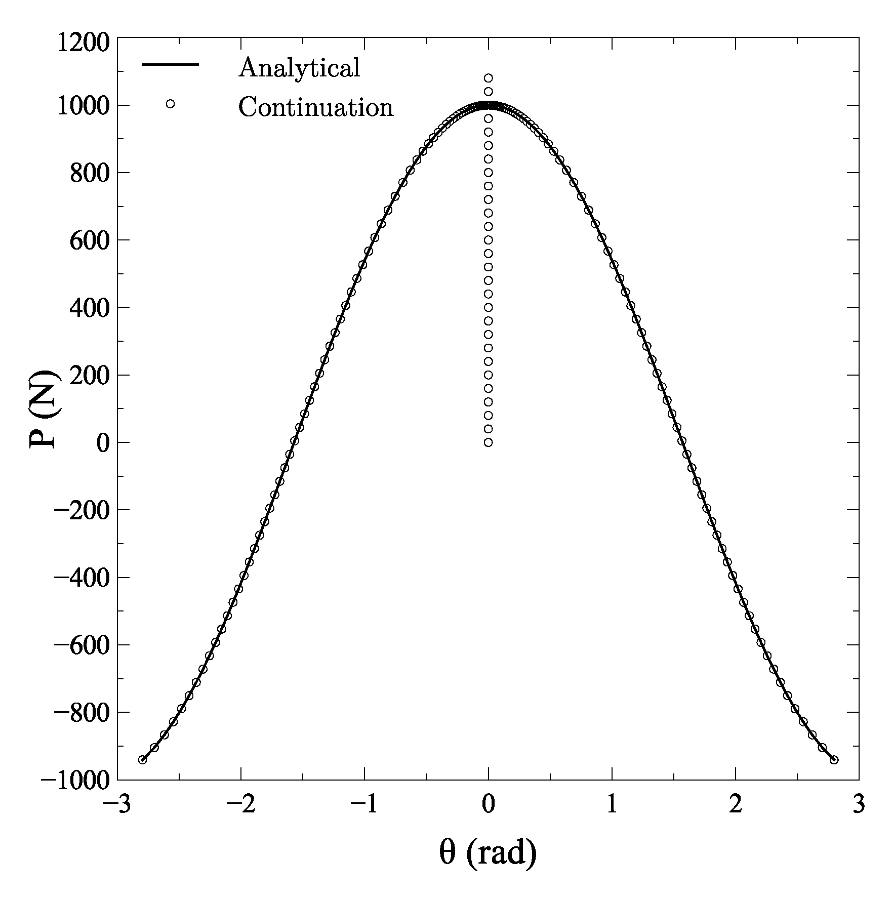
Figure 4.
Cantilever beam with end compressive load.
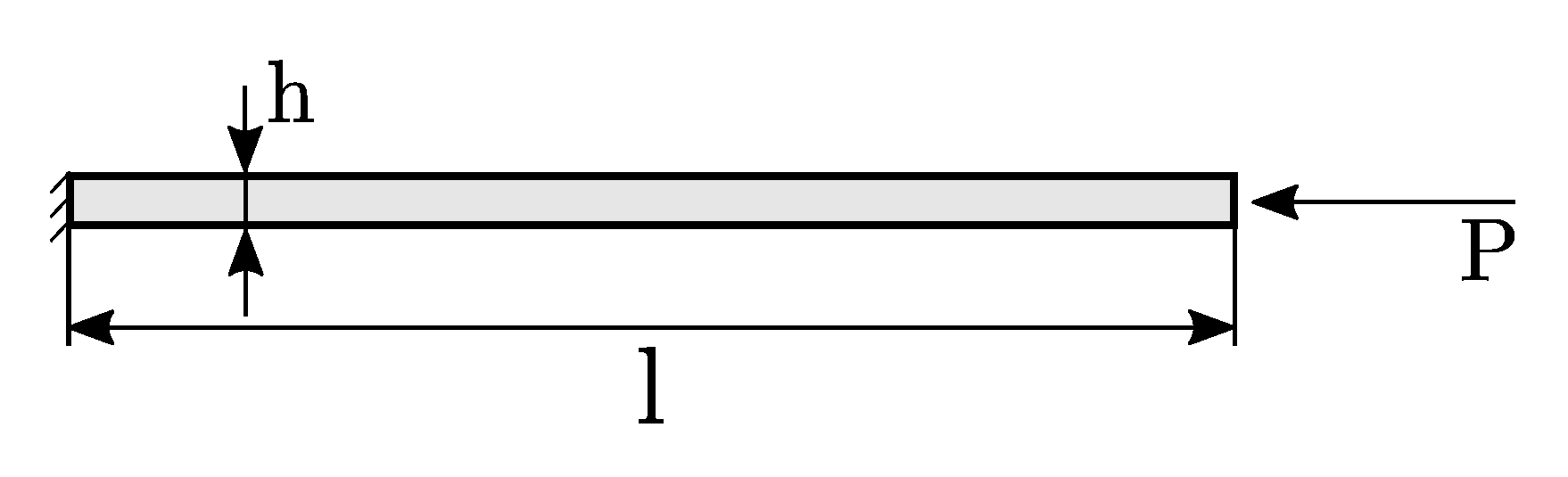
Figure 5.
Bifurcation plot for axially compressed column.

Figure 6.
Beam with initial crack.

Figure 7.
Primary equilibrium path: (a) detection of the first critical point, (b) full equilibrium path.
Figure 7.
Primary equilibrium path: (a) detection of the first critical point, (b) full equilibrium path.

Figure 8.
Computation of the first bifurcation branch: (a) positive side of the branch, (b) corresponding deformed shape, (c) negative side of the branch, (d) corresponding deformed shape.
Figure 8.
Computation of the first bifurcation branch: (a) positive side of the branch, (b) corresponding deformed shape, (c) negative side of the branch, (d) corresponding deformed shape.
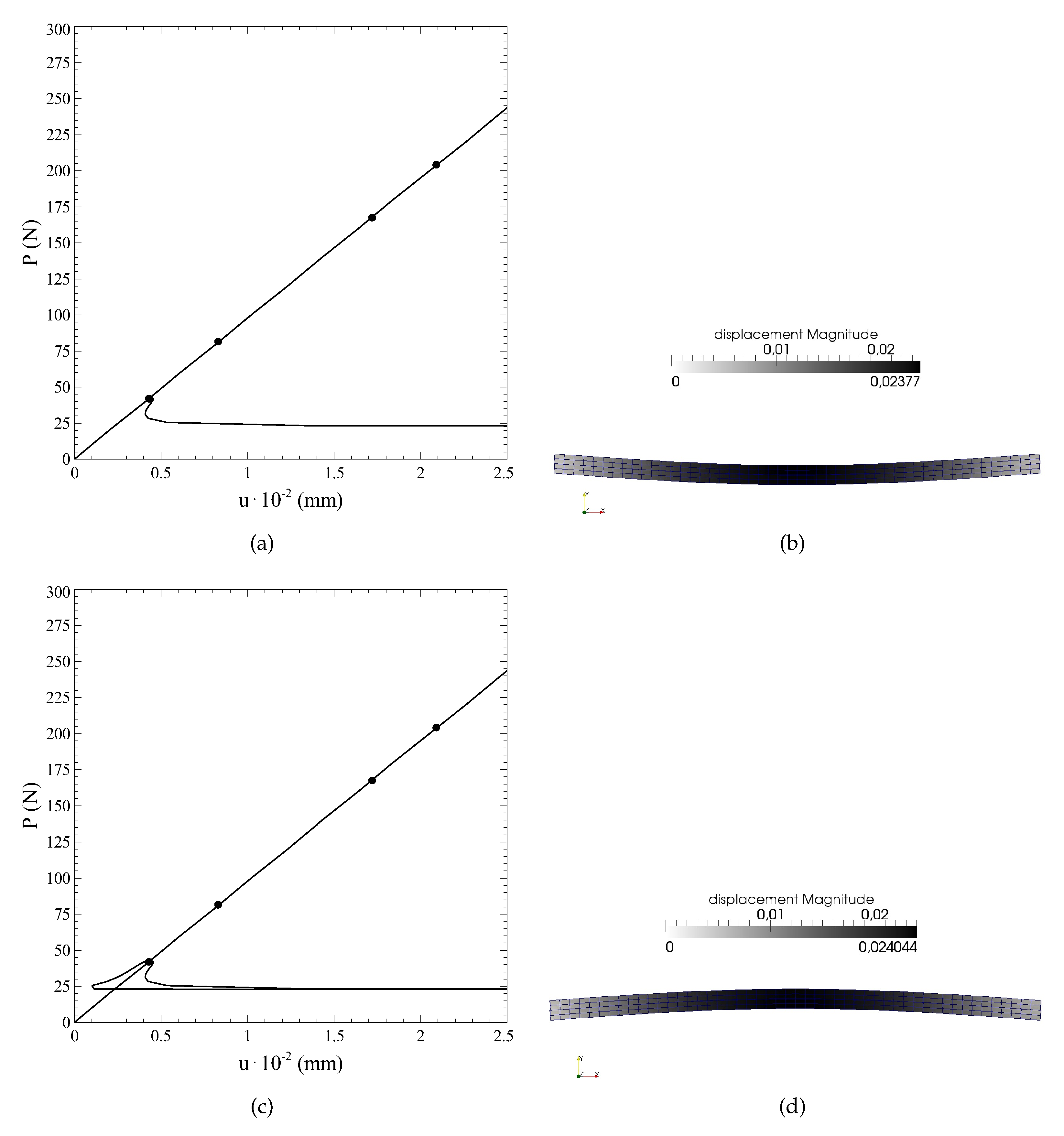
Figure 9.
Computation of the fourth bifurcation branch: (a) positive side of the branch, (b) corresponding deformed shape, (c) negative side of the branch, (d) corresponding deformed shape.
Figure 9.
Computation of the fourth bifurcation branch: (a) positive side of the branch, (b) corresponding deformed shape, (c) negative side of the branch, (d) corresponding deformed shape.
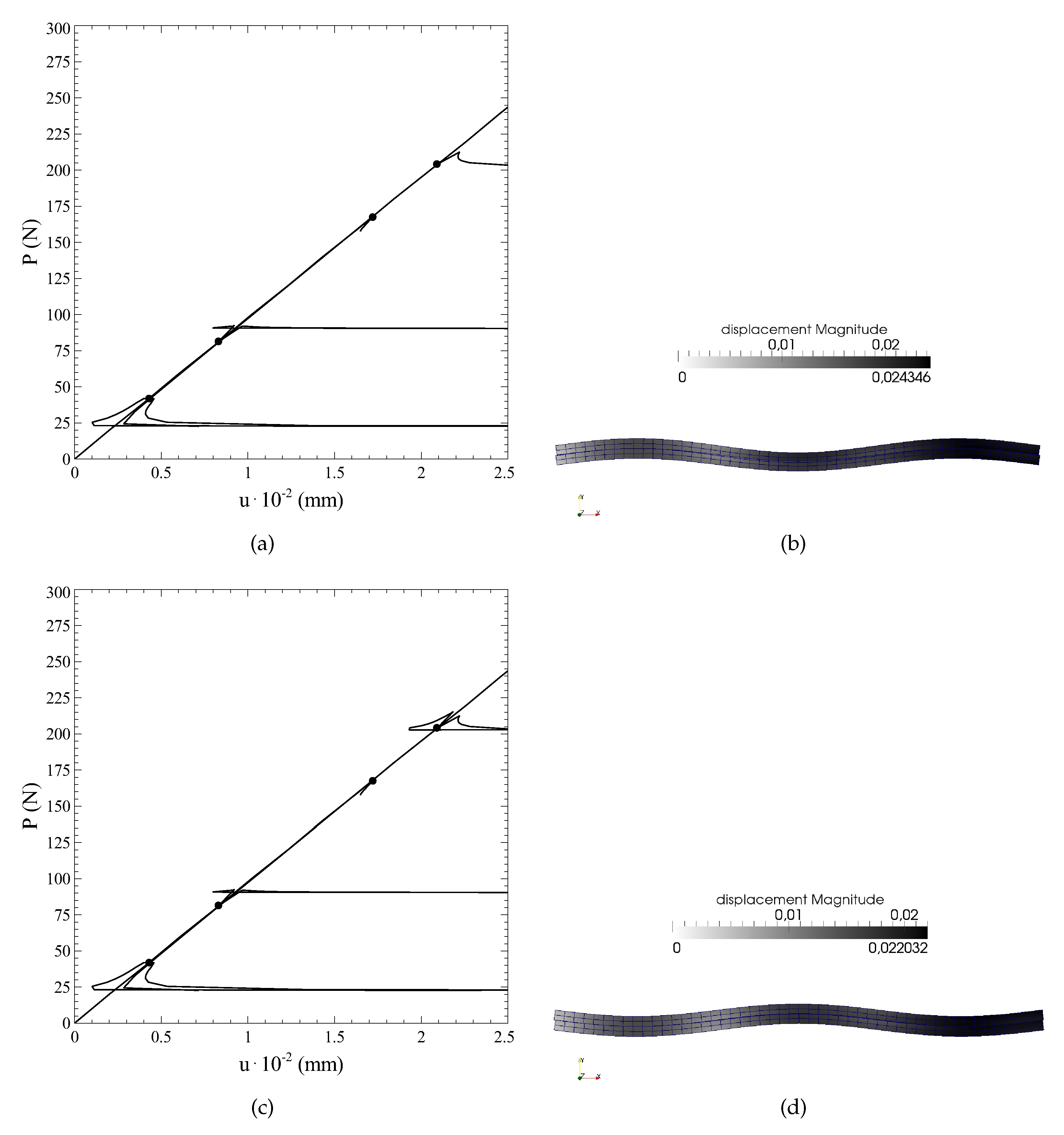
Figure 10.
Post-critical deformed shapes along the equilibrium paths 1 to 4: (a) path 1, (b) path 2, (c) path 3, (d) path 4.
Figure 10.
Post-critical deformed shapes along the equilibrium paths 1 to 4: (a) path 1, (b) path 2, (c) path 3, (d) path 4.

Figure 11.
Detail of the force-displacment curve for the equilibrium branch 3.
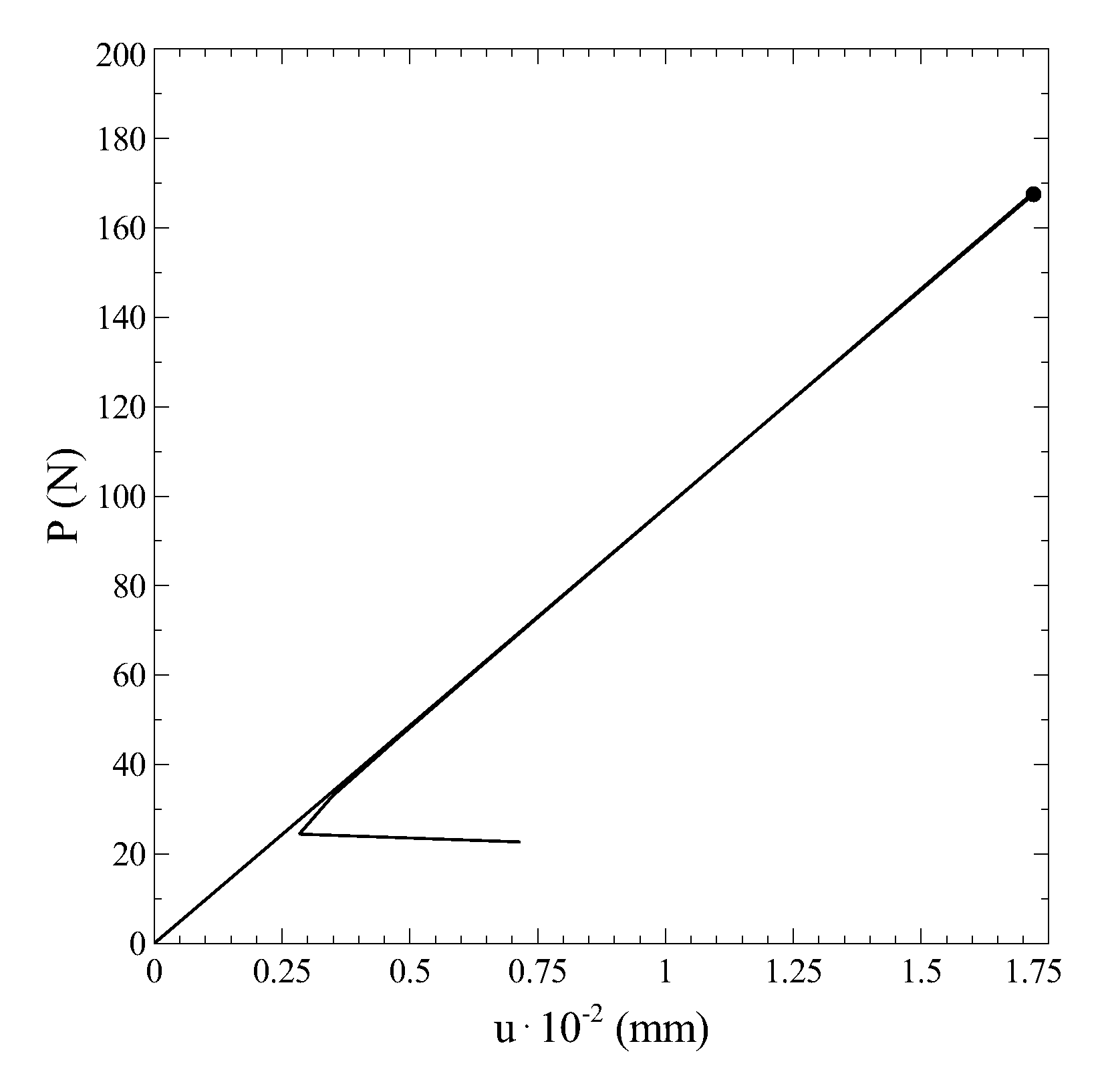
Figure 12.
Arch subjected to distributed pressure.

Figure 13.
Bifurcation plot of the arch subjected to distributed pressure.
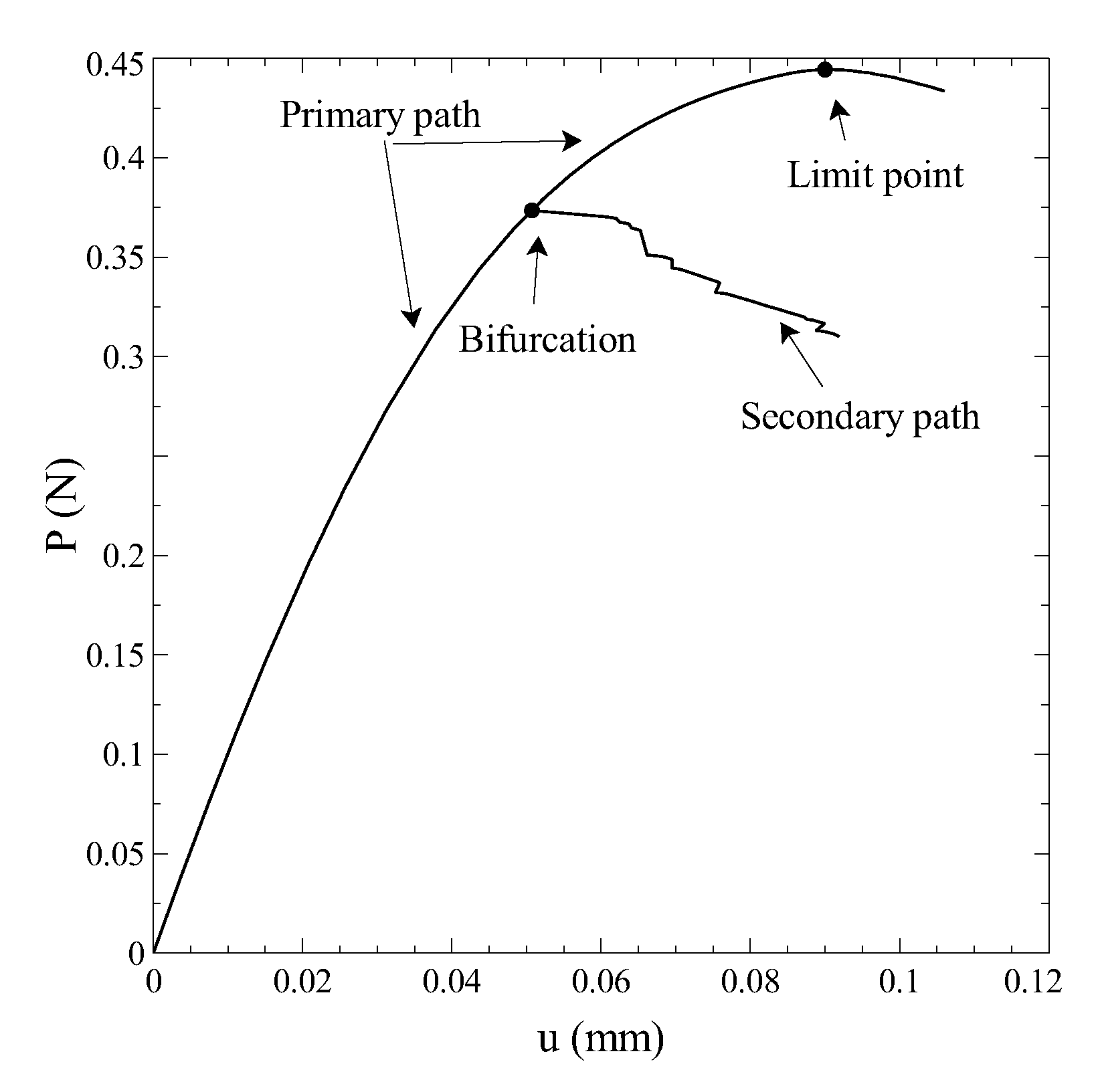
Figure 14.
Cantilever perforated beam: geometry and dimensions.

Figure 15.
Force-displacement curve using different constraints.

Figure 16.
Deformed configuration at the end of the analysis by using: (a) geometric constraint, (b) hybrid constraint.
Figure 16.
Deformed configuration at the end of the analysis by using: (a) geometric constraint, (b) hybrid constraint.


Table 1.
Number of increments using different constraint equations. ( in the parenthesis).
| Constraint | N. of Incr. | N. of Iter. | |||||
|---|---|---|---|---|---|---|---|
| Primary | Branch 1 | Branch 2 | Branch 3 | Branch 4 | Tot | Tot | |
| Hybrid | 10 | 18 (10) | 90 (10) | 35 (50) | 40 (20) | 193 | 332 |
| Geometric | 15 | 40 (10) | 22 (10) | 38 (20) | 31 (30) | 146 | 150 |
Table 2.
Number of increments using different constraint equations. ( in the parenthesis).
| Constraint | N. of Incr. | N. of Iter. | ||
|---|---|---|---|---|
| Primary | Branch 1 | Total | ||
| Hybrid | 47 | 160 (20) | 207 | 276 |
| Geometric | 47 | 160 (30) | 207 | 445 |
Table 3.
Summary of numerical performance for the perforated cantilever beam.
| Constraint | N. of Incr. | N. of Iter. | Step Cuts | N. of Fully Damaged Coh. Els |
|---|---|---|---|---|
| Geometric | 17 | 59 | 3 | 2 |
| Hybrid | 35 | 85 | 1 | 12 |
© 2019 by the authors. Licensee MDPI, Basel, Switzerland. This article is an open access article distributed under the terms and conditions of the Creative Commons Attribution (CC BY) license (http://creativecommons.org/licenses/by/4.0/).
Share and Cite
MDPI and ACS Style
Bellora, D.; Vescovini, R. A Continuation Procedure for the Quasi-Static Analysis of Materially and Geometrically Nonlinear Structural Problems. Math. Comput. Appl. 2019, 24, 94. https://doi.org/10.3390/mca24040094
AMA Style
Bellora D, Vescovini R. A Continuation Procedure for the Quasi-Static Analysis of Materially and Geometrically Nonlinear Structural Problems. Mathematical and Computational Applications. 2019; 24(4):94. https://doi.org/10.3390/mca24040094
Chicago/Turabian StyleBellora, Davide, and Riccardo Vescovini. 2019. "A Continuation Procedure for the Quasi-Static Analysis of Materially and Geometrically Nonlinear Structural Problems" Mathematical and Computational Applications 24, no. 4: 94. https://doi.org/10.3390/mca24040094