Article

Satellite-Based Estimation of Daily Ground-Level PM2.5 Concentrations over Urban Agglomeration of Chengdu Plain

School of Automation Engineering, University of Electronic Science and Technology of China, Chengdu 611731, China
*
Author to whom correspondence should be addressed.
Atmosphere 2019, 10(5), 245; https://doi.org/10.3390/atmos10050245
Submission received: 11 March 2019 / Revised: 22 April 2019 / Accepted: 28 April 2019 / Published: 3 May 2019

Abstract

:
Monitoring particulate matter with aerodynamic diameters of less than 2.5 μm (PM2.5) is of great importance to assess its adverse effects on human health, especially densely populated regions. In this paper, an improved linear mixed effect model (LMEM) was developed. The model introduced meteorological variable, column water vapor (CWV), which has as the same resolution as satellite-derived aerosol optical thickness (AOT), to enhance PM2.5 estimation accuracy by considering spatiotemporal consistency of CWV and AOT. The model was implemented to urban agglomeration of Chengdu Plain during 2015. The results show that model accuracy has been improved significantly compared to linear regression model (R2 = 0.49), with R2 of 0.81 and root mean squared prediction error (RMSPE) of 15.47 μg/m3, mean prediction error (MPE) of 11.09 μg/m3, and effectively revealed the characteristics of spatiotemporal variations PM2.5 level across the study area: The PM2.5 level is higher in the central and southern areas with dense population, while it is lower in the northwest and southwest mountain areas; and the PM2.5 level is higher during autumn and winter, while it is lower during spring and summer. The product data in this paper are valuable for local government pollution monitoring, public health research, and urban air quality control.

Graphical Abstract

1. Introduction

PM2.5, particulate matter with aerodynamic diameters of less than 2.5 μm, is a significant indicator of air pollution level, which has aroused the attention of environmental protection authorities from central and local government in China. Numerous epidemiological studies have demonstrated that there are strong association between PM2.5 exposure and public illness and mortality from respiratory and cardiovascular diseases [1,2,3,4,5,6,7,8,9]. Ground-based monitoring sites can measure PM2.5 level continuously in the long term, but the monitoring sites are generally distributed sparsely and unevenly due to geological and environmental condition restriction, accordingly causing dense distribution in urban area and spare in rural area. Ground-based monitoring networks are inadequate to analyze fine-scale spatial variability of pollution, which is important for health impact assessment and needed to characterize the heterogeneity of human exposure to PM2.5, and effectively prevent and control air pollution [10]. There are many publications that highlight the problem of sparse PM2.5 locations. Let us start with the review paper of Hoff and Christopher 2009 [11].
However, aerosol optical thickness (AOT), one parameter of the characteristics of aerosol, is equal to the integral extinction coefficient over a vertical column of atmosphere at observation location, and it represents the degree to which aerosol prevent the transmission of light by absorption or scattering of light. AOT can be derived from satellite imageries indirectly [12,13,14,15], and numerous global satellites are widely used for AOT retrieval, e.g., advanced very high-resolution radiometer (AVHRR), total ozone mapping spectrometer (TOMS), moderate-resolution imaging spectroradiometer (MODIS), multi-angle imaging spectroradiometer (MISR), sea-viewing wide field-of-view sensor (SeaWifFS) [16], and visible infrared imaging radiometer suite (VIIRS) [17], continuously measuring AOT from the late 1990s to the most recent.
Satellite data are able to monitor large/urban scale air quality through adding synoptic and spatial distribution information to ground-based air quality measurements and modeling [18,19]. In recent decades, numerous researchers have developed many algorithms for calibrating satellite-derived AOT to ground-level PM2.5 concentrations. Early studies primarily established simple linear regression models to relate PM2.5 and AOT [19,20,21]. Then, meteorological data were incorporated in the multiple regression analysis and improved the PM2.5–AOT correlation [22]; advanced statistical models, such as artificial neural networks (ARN) [23], generalized additive model (GAM) [24,25], land use regression model (LUR) [26,27,28], and geographically weighted regression (GWR) [29,30,31,32,33] were developed to analyze the variability of PM2.5–AOT relationship correlated with meteorology or land use data. Although such advanced models gained higher estimation accuracy for large regions such as the northeastern and southeastern US, Europe, and China, etc., auxiliary parameters increased the complexity of these models and introduced other errors. Lee firstly incorporated time-varying parameters (day-to-day) in a statistical model to calibrate MODIS AOT and obtained good estimation accuracy [34]; and this model was further improved through adding meteorological data, land use data, and pollution sources over the whole China, Beijing, Beijing–Tianjin–Hebei (BTH) region, Yangtze River Delta (YRD), Peral River Delta (PRD), California, and southeastern U.S. [33,35,36,37,38,39,40,41,42,43,44,45].
In the presence of water in the atmosphere, an aerosol particle changes its size and other characteristics by absorbing or evaporating water (i.e., aerosol hygroscopic growth) [46]. Because AOT is an indicator of the abundance of aerosol particles in the total vertical column while PM2.5 concentration is measured at ground level, the correlation between them is influenced by the vertical distribution of aerosols and the humidity that impacts aerosol extinction coefficient. These two factors are associated with atmospheric profiles, ambient conditions, as well as the size distributions and aerosol particles components, all of which may have large spatial and temporal variations. Hence, PM2.5 estimates from AOT alone will have large uncertainties. To reduce these uncertainties, numerous studies have incorporated the planetary boundary layer height, ambient relative humidity, and other meteorological factors (e.g., temperature, wind speed) in their models to better characterize the correlation between AOT and PM2.5 [21,22,24,29,32,33,37,38,39,42,47,48,49]. However, it is usually difficult to obtain those observational parameters, such as particle vertical distribution at specific locations. Most of the works mentioned above were conducted using data obtained from the sparse ground-based monitoring sites [33,38,47,48] and model assimilated meteorological data, e.g., Goddard earth observation system data assimilation system [21,39,42], rapid update cycle [22,24] North American regional reanalysis [29], European Center for Medium-Range Weather Forecasts [32], and North American land data assimilation system [37]. Because of the establishing strategies of ground-based monitoring sites, there are very few, even no, monitoring sites in exurban and rural areas, small towns, etc., which may cause some uncertainties in model retrieval. Meanwhile, model-assimilated meteorological data can have better spatial coverage over all the locations, but their grid spatial resolution is low such as 0.25° latitude × 0.3125° longitude and 13 km, which are much lower than that of satellite AOT, causing serious inconsistence of spatial coverage between meteorological data and AOT grid cell. As discussed above, many meteorological variables can substantially affect the PM2.5–AOT relationship and are significant predicators of PM2.5 concentrations, and the meteorological data source also introduces some uncertainties.
Conventional Collection 5.1 (C5.1) MODIS AOT at 10 km spatial resolution and Collection 6.0 (C6) MODI AOT at 3 km spatial resolution were widely used to estimate ground-level PM2.5 concentration due to its daily global coverage and availability in the long term. Nevertheless, those spatial resolutions are not enough to capture the spatial variation of air pollution in urban scale [50,51].The multi-angle implementation of atmospheric correction (MAIAC) algorithm were developed for the MODIS aerosol retrievals and atmospheric correction over both dark vegetated surfaces and bright deserts based on a time series analysis and image-based process, producing products such as AOT, spectral regression coefficient (SRC), column water vapor (CWV), and bidirectional reflectance distribution function (BRDF) at 1 km spatial resolution, which is finer than previous MODIS AOT products [52,53]. More importantly, the MAIAC CWV is generated along with MAIAC AOT from MAIAC algorithm, so both of them have the same spatial coverage and time taken.
In this study, in order to reduce the uncertainty caused by inconsistency of spatiotemporal between AOT and meteorological data, we firstly incorporated MAIAC CWV into PM2.5 estimation model based on widely used LMEM method [34]; and the model is implemented to urban agglomeration of Chengdu Plain, which is one of the most heavily polluted in China in 2015 [54,55,56]; then, we assessed model performance via different ground measurements of PM2.5 datasets and MAIAC AOT datasets; the spatiotemporal change of PM2.5 level in urban agglomeration of Chengdu Plain was also analyzed. A final table with acronyms is attached at the end of the manuscript, please see Appendix A.

2. Materials and Methods
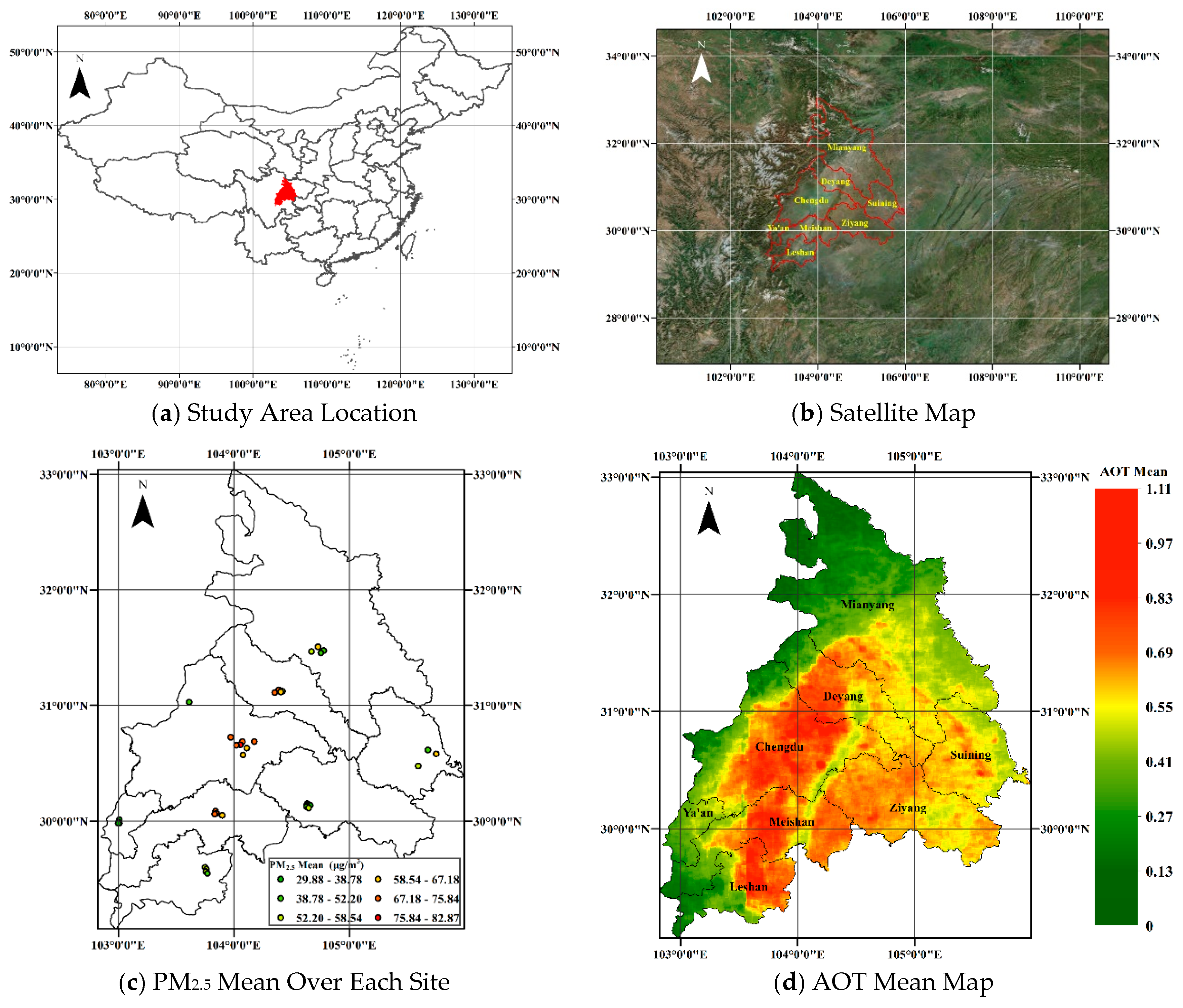
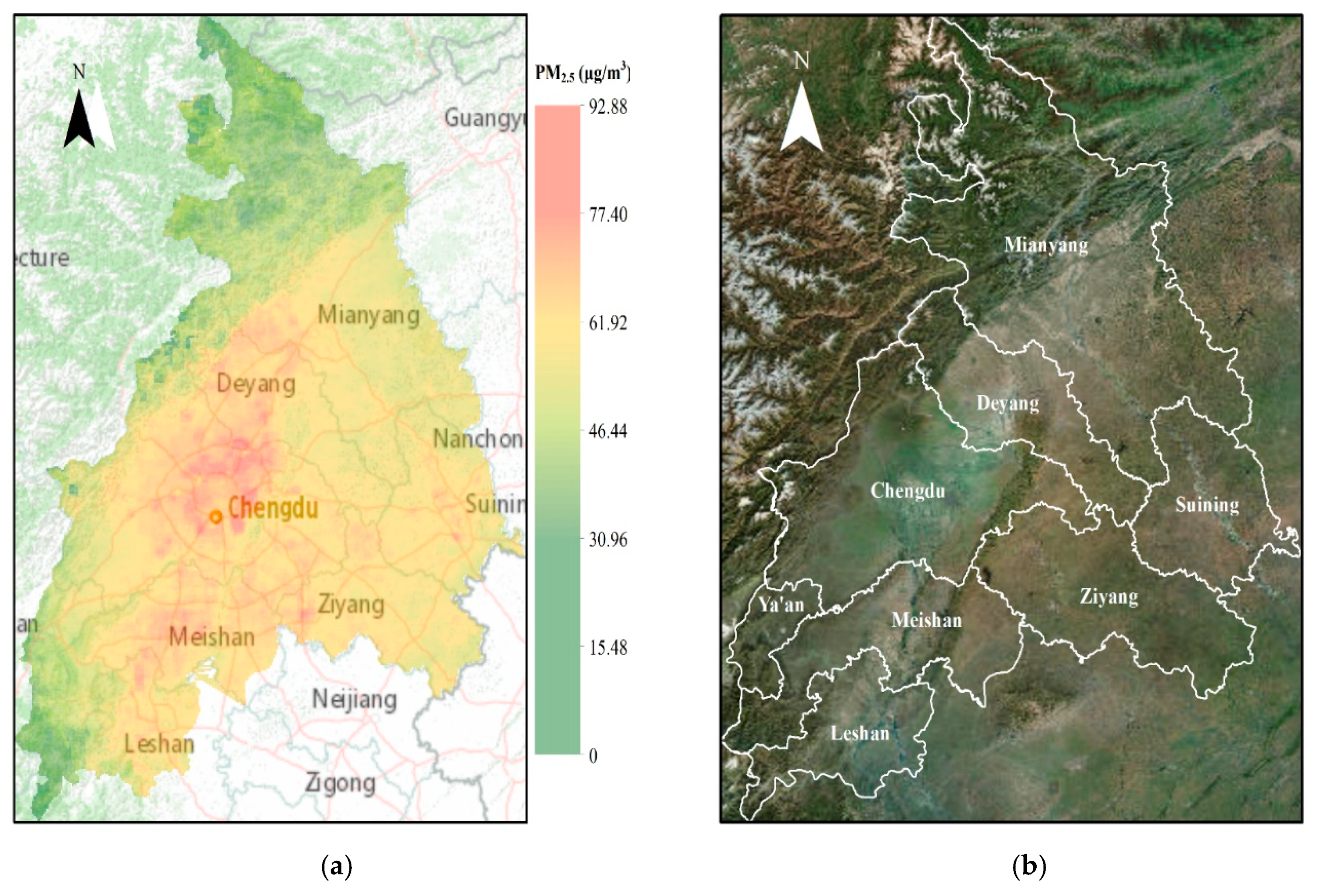
2.1. Study Area

The urban agglomeration of Chengdu Plain consists of 8 province-controlled cities: Chengdu, Deyang, Mianyang, Meishan, Ziyang, Suining, and part of Ya’an and Leshan, with a population of around 50 million. It is located in the western part of the Sichuan Basin surrounded by mountains: The Longmen Mountains lie in the northwest, the Qionglai Mountains lie west, and the Longquan Mountains lie east (Figure 1b). Due to the surrounding mountains and temperature inversion, it often experiences foggy weather and smog. The climate has distinct seasons but is moist and cloudy, with the least days of sunshine in China. In recent years, it has undergone heavy air pollution because of the enormous economic boom, urban construction, the increase in the number of motorized vehicles, population growth, surrounding topography, and seasonal weather conditions.

2.2. Ground-Level PM2.5 Datasets

Ground-level PM2.5 datasets are used for model fitting and model testing in our study. PM2.5 data are collected hourly from 36 monitoring sites of national monitoring networks in urban agglomeration of Chengdu Plain (Figure 1c and see Supplementary: Table S1). The ground-based PM2.5 monitoring sites are deployed densely in urban area and sparsely in rural area and measured by the tapered element oscillating microbalance method (TEOM) [49,57], which has an accuracy of ±1.5 μ g / m 3 for 1 h average, and performs a calibrating process and quality control according to the Chinese National Ambient Air Quality Standard (China NAAQS) [58]. The TEOM continuously pumps in the ambient air and heats it up (to remove the water vapor’s influence), and the particles with sizes smaller than 2.5 μm are selected by passing through a special head and then weighted. Thus, the dry mass of PM2.5 within a unit volume of ambient air is acquired and recorded every 15 min. It should be noted that by heating the air sample, the measured PM mass (dry) might be less than the real PM level in the ambient air due to the volatilization of semi-volatile aerosol components [59].
In order to better explore the PM2.5–AOT relationship, we selected four PM2.5 datasets, which are mainly based on two satellites (i.e., Terra and Aqua) overpass. AOTs are measured by Terra satellite (at ~10:30 local time) in the morning and Aqua satellite (at ~13:30 local time) in the afternoon. The four PM2.5 datasets are averaged from hourly ground-level PM2.5 at different time period: 1) PM2.5 24-h average; 2) PM2.5 time average of 10:00 and 14:00; 3) PM2.5 time average of 10:00 and 11:00; 4) PM2.5 time average of between 13:00 and 14:00 at each monitoring site in 2015.

2.3. MAIAC Product Datasets

In our study, the MAIAC product was downloaded for both Terra and Aqua from National Aeronautics and Space Administration (NASA) Center for Climate Simulation via https portal [60]. In order to maintain reasonable file size, the MAIAC algorithm team divided the entire China up into a title grid, and the title grid coordinate system starts at (0, 0) (horizontal tile number, vertical tile number) in the upper left corner and proceeds right (horizontal) and downward (vertical). The study area consists of two tiles, i.e., h02v02 and h03v02. The two tiles include MAIAC data derived from both Terra satellite in the morning and Aqua satellite in the afternoon. The MAIAC algorithm was specifically developed for MODIS data, performing aerosol retrievals and atmospheric correction over both vegetated surfaces and bright deserts at 1 km spatial resolution based on time-series analysis and image-based processing [52,53]. MAIAC algorithm generates products such as aerosol parameters, CWV, BRDF, and SRC. The aerosol parameters include AOT, fine mode fraction, Angstrom exponent from wavelength of 0.47 to 0.67 um, and aerosol type including background, smoke, and dust models [53]. Firstly, MAIAC collected an accumulation of MODIS observations during 5 (over poles)–16 (over equator) with a sliding window approach at specific region. Then, those MODIS data were gridded to 1 km spatial resolution with specific projection coordinate system. When the surface remains stable during collection period, the surface BRDF is retrieved using the regional background aerosol model. Because the 2.1 μm band is transparent to aerosol, it is used to retrieve aerosol and surface reflectance over dark and moderately bright surfaces. Four or more days with low AOT values are used to calculate SRC correlating surface reflectance in the blue and shortwave infrared bands. Once SRC is obtained, the AOT is retrieved with the last MODIS observation. AOT retrieval is conducted with the regional background aerosol model in clear conditions, and surface BRDF in haze conditions. Aerosol robotic network (AERONET) [61] validation shows that the MAIAC and MOD04 algorithms have similar accuracy over dark and vegetated surfaces and have improved the accuracy over brighter surfaces due to SRC retrieval and BRDF factor characterization, as demonstrated for several U.S. west coast AERONET sites [53].
Due to cloudy and foggy weather conditions in the study area, there are many days or areas without satellite AOT measurements. In order to improve spatial coverage of satellite-derived AOT, we merged MAIAC AOT measurements of the Terra satellite (at ~10:30 local time) in the morning and Aqua satellite (at ~13:30 local time) in the afternoon [35,42]. With regard to a given location in one day, there are two situations for AOT availability, one in which both MAIAC Aqua AOT and MAIAC Terra AOT are available, and the other in which just one of MAIAC Aqua AOT and MAIAC Terra AOT is available. If the two AOT measurements (i.e., Terra and Aqua) have strong correlation, we can estimate missing AOT measurement form each other. Hence, in our study, we developed a simple linear regression model with MAIAC Terra AOTs and MAIAC Aqua AOTs in the first situation, then estimate missing AOT measurements from another available one in the second situation. Since the ratio of AOT in the morning to that in the afternoon varied by season, we classified one year into two seasons: Warm season (March to August) and cold season (September to February). The linear regression models of estimating missing AOTs in different season in our study were given as below:
Warm season:
τ T e r r a = 0.899 τ A q a u a + 0.080
τ A q u a = 0.885 τ T e r r a + 0.028
Cold season:
τ T e r r a = 1.025 τ A q u a + 0.046
τ A q u a = 0.869 τ T e r r a + 0.025
where τ is the MAIAC AOT value. The R2 of regression models on warm season and cold season were 0.80 and 0.89, respectively. The missing AOT value was estimated using the above regression equation and then the daily AOT was calculated by averaging of MAIAC Terra AOT and MAIAC Aqua AOT. Finally, the daily AOT represents the average aerosol level between 10:00 and 14:00 for each day.
We also evaluated the MAIAC AOT product. Because there is no AERONET site in Sichuan Basin, the ground-based AOT measurements from three AERONET sites in Beijing (Beijing [116.38° E, 39.97° N], Beijing_CAMS [116.31° E, 39.93° N], and Beijing_RADI [116.37° E, 40.00° N]) in the year of 2015 were used to validate the MAIAC AOT. To be comparable with the spectrum setting of MODIS, AERONET AOT at 550 nm were gained by calculating the Angstrom turbidity coefficient and Angstrom exponent with AEROENT measured AOTs at two wavelengths (440 nm and 675 nm) [62,63]. The total number of AOT pairs (MAIAC AOT–AERONET AOT) for the three sites are 257, 272, and 90, respectively. MAIAC AOT shows high temporal correlation with AERONET AOT (see Supplementary: Figure S1), with Pearson correlation coefficients R of 0.96, 0.97, and 0.97 at three sites, respectively, and the mean AOT difference MAIAC and AERONET at three sites is 0.097.

2.4. Population Datasets

The gridded population of the world (GPW) collection in fourth version (GPWv4) generated by socioeconomic data and application center (SEDAC) was used in our study. It can provide a spatially disaggregated population layer that is compatible with datasets from social, economic, and remote sensing. GPWv4 used the results of the 2010 round population and housing censuses with much finer spatial resolution. It produces the population distribution for the years 2000, 2005, 2010, 2015, and 2020 [64]. In this study, GPW data in 2015 at 1 km spatial resolution were employed. In our study, min-max normalization process was also performed to change the range of GPW data ranging from 0 to 1.

2.5. Data Pre-Processing and Matching

To establish the PM2.5-AOT relationship model (parameterization), the ground-based daily PM2.5 measurements, gridded population data (POP), satellite-derived MAIAC AOT, and CWV values must be collected at the closest spatial location and time. For each monitoring site (PM2.5), the 1 km pixel of MAIAC AOT, CWV, and POP where the monitoring site location is selected. The PM2.5, AOT, CWV, and POP is picked to form a sample PM2.5-AOT pair. Data pairs with either PM2.5 values less than 3.0 μg/m3 or missing PM2.5/AOT measurements are omitted. In addition, because the regression slope cannot be estimated from only one single data pair, the days with less than two PM2.5-AOT pairs available are excluded.

2.6. LMEM Model Fitting and Validation

Lee et al. [34] established day-specific PM2.5–AOT relationships using LMEM algorithm and estimated daily estimation of ground-level PM2.5 concentrations based on MOD04 AOT in the New England region, considering the day-to-day variability of PM2.5–AOT relationship correlated to mixing height, relative humidity, PM2.5 composition, and PM2.5 vertical profile with the assumption that PM2.5–AOT relationship varies largely day to day but minimally spatially on a given day in study area. The LMEM calculates day-specific random intercepts and slopes for the PM2.5–AOT relationship and incorporates both fixed-effects terms and random-effects terms. As discussed above, the correlation between PM2.5 and AOT is influenced by the humidity that affects aerosol extinction coefficient. Because the aerosol vertical profile during satellite (Terra and Aqua) overpass time in each day is difficult to obtain, the model did not take it into account. Moreover, anthropogenic factors influencing the PM2.5–AOT relationship usually are constant, e.g., major road, factory emissions. Hence, we incorporated population data as another indicator of influencing the spatial variability of the PM2.5–AOT relationship. It is should be noted that to reduce the uncertainty caused by inconsistency of spatiotemporal between AOT and meteorological data, both of them are should be generated from the same satellite. The improved LMEM equation is below:
PM ij = ( α + μ j ) + ( β + υ j ) × AOT ij + ( γ + φ j ) × CWV ij + P O P i + ε ij
where, PM ij is the daily average PM 2.5 concentration (μg/m3) at site i on day j; AOT ij is the daily average AOT value (unitless) corresponding to site i on day j; CWV ij is the daily average CWV value (cm) corresponding to site i on day j; P O P i is the population over the area covering the site i; α and μ j are the fixed and random intercepts on day j, respectively; β and υ j are the fixed and random slopes for AOT on day j, respectively; γ and φ j are the fixed and random slopes for CWV on day j, respectively; ε ij is the error term at site i on day j. In this model, the fixed parameter β and γ of AOT and CWV represent the average effects on PM2.5 concentrations for the entire space and time in the study area, while the random parameter υ j and φ j (day-specific) explain daily variation of the PM2.5-AOT relationship. The above statistical model (Equation (5)) was applied to the entire sample pairs of PM2.5–AOT to calculate the fixed-effect intercept and slope for all the model-valid days and random effect intercepts and slopes (day-specific) for each individual model-valid day. Finally, we get PM2.5 estimation model for each model-valid day. The model coefficients were calculated using package ‘lme4’ of R programming language (version 3.4.3).
For model validation, 10-fold cross-validation (CV) [65] was applied to test the model potential over-fitting through randomly dividing the entire sample pairs (i.e., PM2.5–AOT pair) into 10 subsets with almost 10% of the whole sample pairs for each subset. The process of CV was conducted through using nine sample subsets for model fitting, while the remaining one sample subset for model testing, then repeated 10 times until every subset was tested and combined all the testing subsets. We assessed the model performance by calculating the overall R2, the site-specific (each site) R2 between PM2.5 estimates and ground ground-based measurements, mean prediction error (MPE), and root mean squared prediction error (RMSPE) for model fitting and CV results.
MPE = i = 1 n ( y i y i ) / n
RMSPE = i = 1 n ( y i y i ) 2 / n
where, y i and y i are the estimated PM2.5 and the measured PM2.5 of the ith sample, respectively, and n is the total number of PM2.5-AOT pair samples.
In this paper, a model that estimates daily ground-level PM2.5 concentrations was established. Using the model, we generated seasonal and yearly averaged PM2.5 concentrations using the daily PM2.5 estimates in the study area across the whole study period.

3. Results

3.1. Data Descriptive Statistics

In our study, in order to increase spatial coverage, the AOT average (daily AOT) of MAIAC Terra AOT (~ 10:00 local time) and MAIAC Aqua AOT (~ 14:00 local time) were used to establish PM2.5 estimation models. We built the linear regression models for warm and cold seasons based on days where both AOT in the morning and AOT in the afternoon are available, then missing AOTs were estimated via above linear models. After adjusting, the size of model fitting dataset was dramatically increased, with PM2.5–AOT sample pairs increased from 529 to 1635 and corresponding model-valid days from 53 to 129 during 2015. Data statistics summary shows that the overall mean of PM2.5 24-h average is 58.25 μg/m3, varying from 29.88 μg/m3 (SD = 15.60 μg/m3) to 82.87μg/m3 (SD = 48.28 μg/m3) by site (see Supplementary: Table S2) and the overall mean of PM2.5 time average of 10:00 and 14:00 is 60.70 μg/m3, varying from 23.86 μg/m3 (SD = 13.24 μg/m3) to 88.35 μg/m3 (SD = 57.3 μg/m3) by site (see Supplementary: Table S3); the overall mean MAIAC AOT is 0.64, varying from 0.39 (SD = 0. 20) to 0.79 (SD = 0.38) by site (Table S4). Figure 1c shows that high PM2.5 level mainly occurs at Chengdu, Deyang, and Meishan, located in the central and south areas of the study area, which might likely be due to high population density, vehicles, climate (high humidity all year), and terrain condition; the MAIAC AOT average (Figure 1d) and PM2.5 levels for the entire study period (Figure 1d) have a similar spatial pattern.

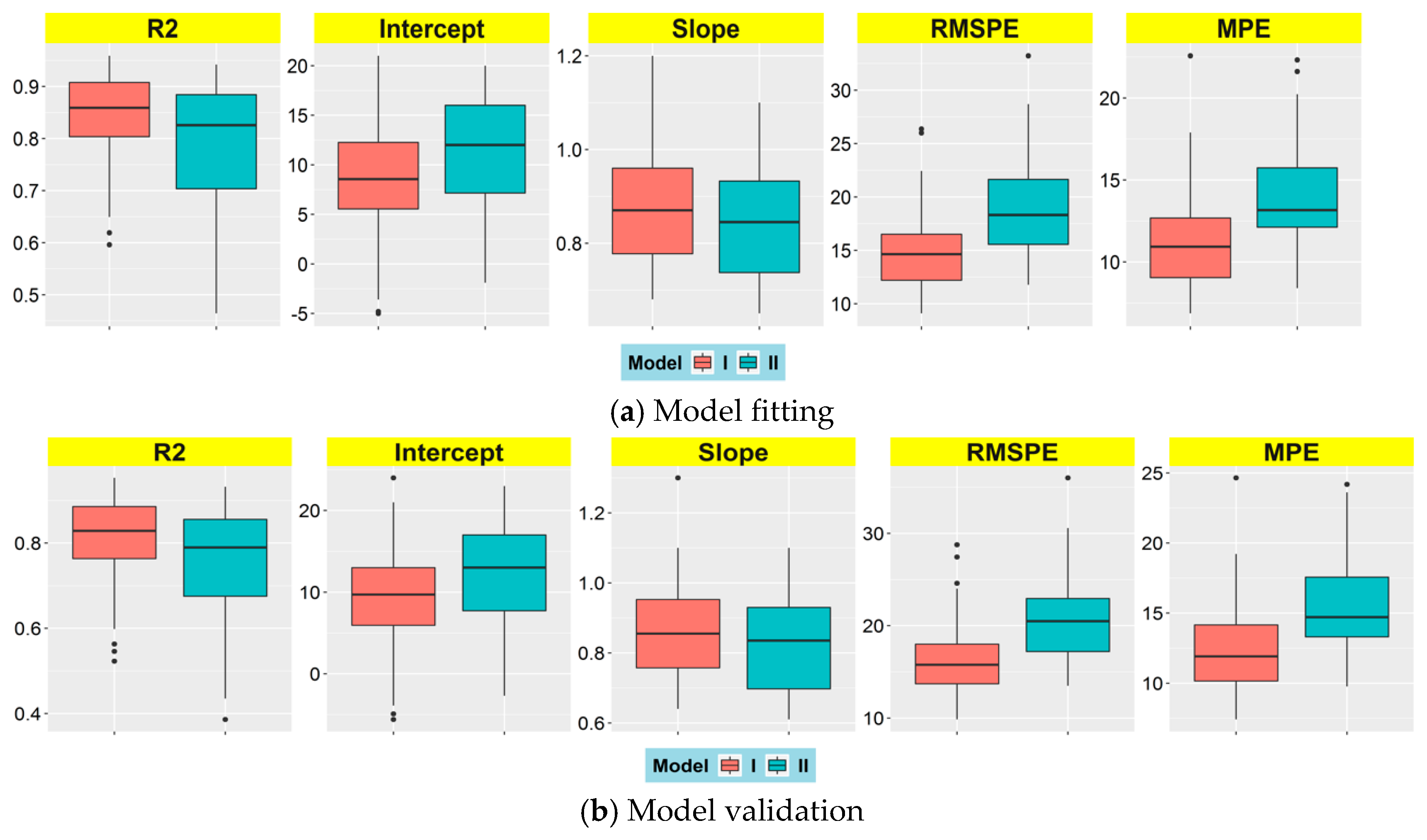
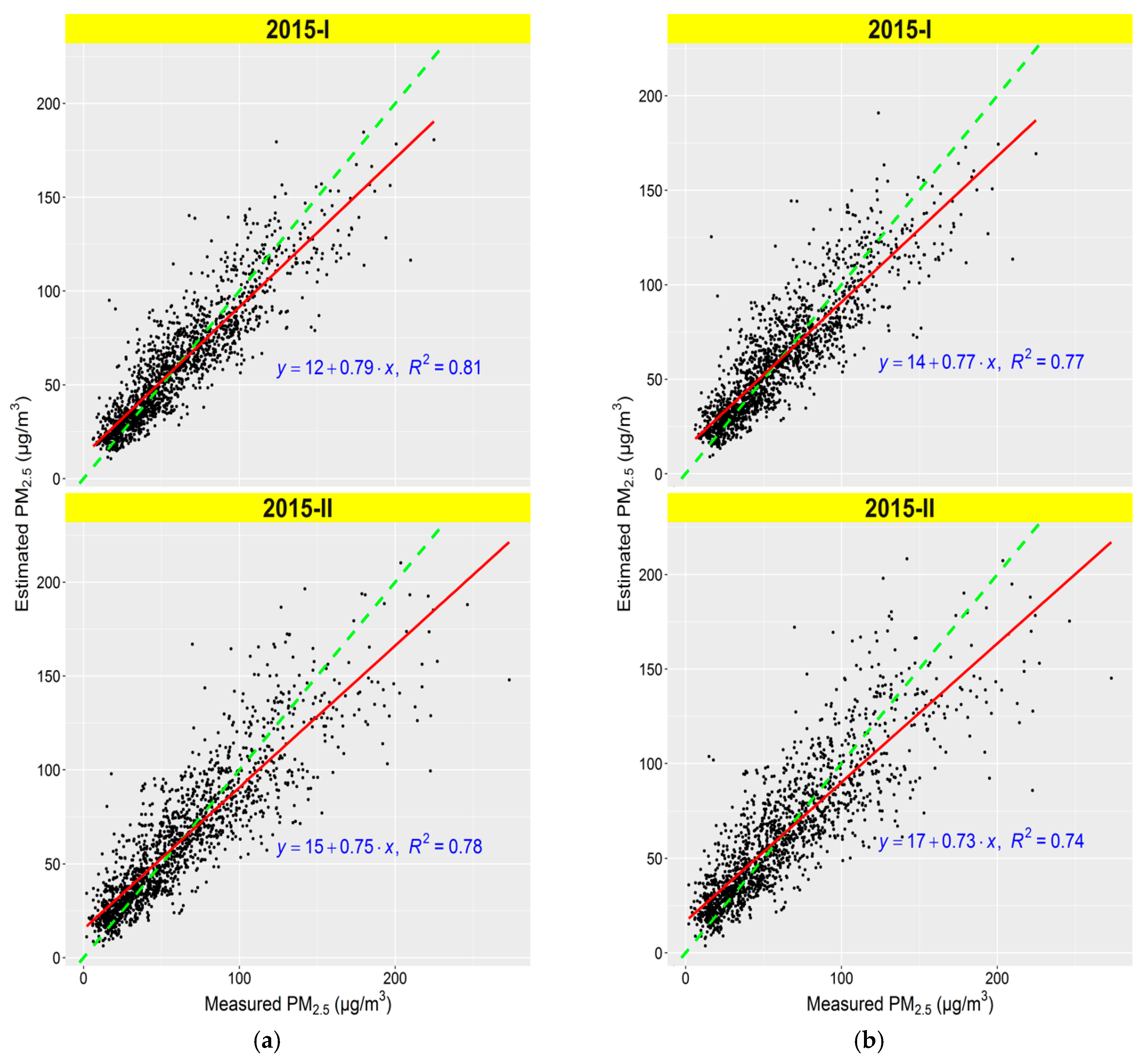
3.2. Results of Model Fitting and Validation

In our study, we established several models for daily estimation of ground-level PM2.5 with different PM2.5 time average datasets and AOT datasets. Firstly, PM2.5 estimation models were fitted using the MAIAC AOT average, PM2.5 24-h average (model-I), and PM2.5 time average of 10:00 and 14:00 (model-II). Based on PM2.5 estimates and ground-based measurements, we calculated R2, intercept, slope, RMSPE, and MPE between them for each monitoring site. Figure 2a shows the boxplots statistics of model fitting performance at all the 36 sites, and site-specific R2 ranges from 0.60 to 0.96, slope is from 0.68 to 1.20, RMSPE is from 9.08 μg/m3 to 26.36 μg/m3, MPE is from 6.86 μg/m3 to 22.57 μg/m3 for Model-I; and R2 ranges from 0.46 to 0.94, slope is from 0.65 to 1.10, RMSPE is from 11.76 μg/m3 to 33.22 μg/m3, MPE is from 8.40 μg/m3 to 22.31 μg/m3 for Model-II; and median values of R2, slope for Model-I (0.84) is higher than corresponding values of Model-II (0.78), while RMSPE has an adverse result (14.88 μg/m3 versus 19.24 μg/m3), indicating that Model-I has much better estimation performance than Model-II, and good agreement between fitted and measured PM2.5 at each monitoring site. The overall R2 of all the sites is 0.81 for Model-I, while it is 0.78 for Model-II. The scatterplots of PM2.5 estimates of model fitting versus ground-based PM2.5 measurements can be seen in Figure 3a. Table 1 shows the mode performance of Model-I and Model-II, demonstrating that both PM2.5 24-h average and PM2.5 time average of 10:00 and 14:00 can be used to fit estimation models with good estimation performance, and among them, model-fitted ith PM2.5 24-h average is much better. In addition, model CV performance statistics results are shown in Figure 2b and Figure 3b; the performance statistics of model CV (Figure 2b) shows that site-specific R2 for both Model-I and Model-II decrease, while RMSPE and MPE increase from model fitting to model validation with small differences. On the other hand, model CV results shown in Figure 3b and Table 1 indicate that overall R2 of Model-I and Model-II are 0.77 and 0.74, respectively, for the entire study period. Both Model-I and Model-II have over-fitting due to R2 decrease and RMSPE and MPE increase, yet the differences are small. Overall, although both Model-I and Model-I have good estimation performance with higher R2 values, Model-I is better due to lower RMSPE and MPE. So, we employed Model-I to estimate daily ground-level PM2.5 concentrations over the study area for all model-valid days in the year of 2015.
In addition, models are also established using just one satellite observation (Table 1), i.e., Model-III fitted with Terra AOT and PM2.5 time average of 10:00 and 11:00, Model-IV fitted with Aqua AOT and PM2.5 time average of 13:00 and 14:00, Model-V fitted with the average of MAIAC Terra AOT and MAIAC Aqua AOT (both of them are available in a given day) and PM2.5 24-h average, and Model-VI fitted with the average of MAIAC Terra AOT and MAIAC Aqua AOT (both of them are available in a given day) and PM2.5 time average of 10:00 and 14:00. It should be noted that the missing AOT is not estimated for Model-V/VI. Model estimation performance of above four models are also given in Table 1, indicating that the model fitted R2 are higher for most models except Mode-III, and Model-V with the highest R2, and lowest RMSPE and MPE. Models fitted with PM2.5 24-h average (Model-I, Model-V) are better than those with PM2.5 time average of 10:00 and 14:00 (Model-II, Model-VI) due to higher R2 and lower RMSPE and MPE. Also, the model fitted with MAIAC Aqua AOT (Model-IV) is better than that with MAIAC Terra AOT (Model-III), with higher R2 and lower RMSPE and MPE but with less model-valid days and PM2.5–AOT sample pairs.
The differences between Model-I estimated and ground-based PM2.5 concentrations are shown in Figure 4. It can be seen that PM2.5 concentrations are slightly overestimated in lightly polluted areas, while underestimated at heavily polluted areas. Nevertheless, the difference were within ± 17.13 μg/m3 for 80% of all the monitoring observations.

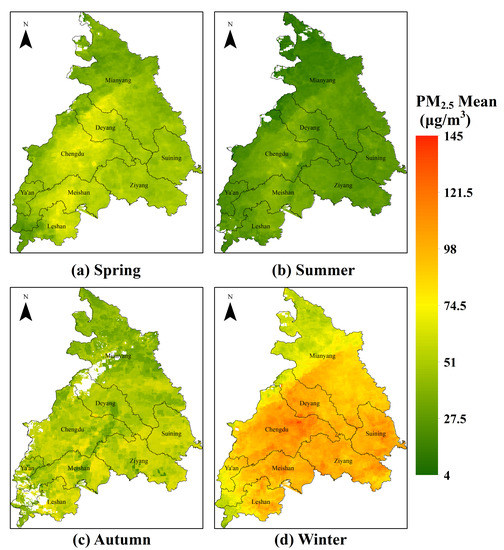
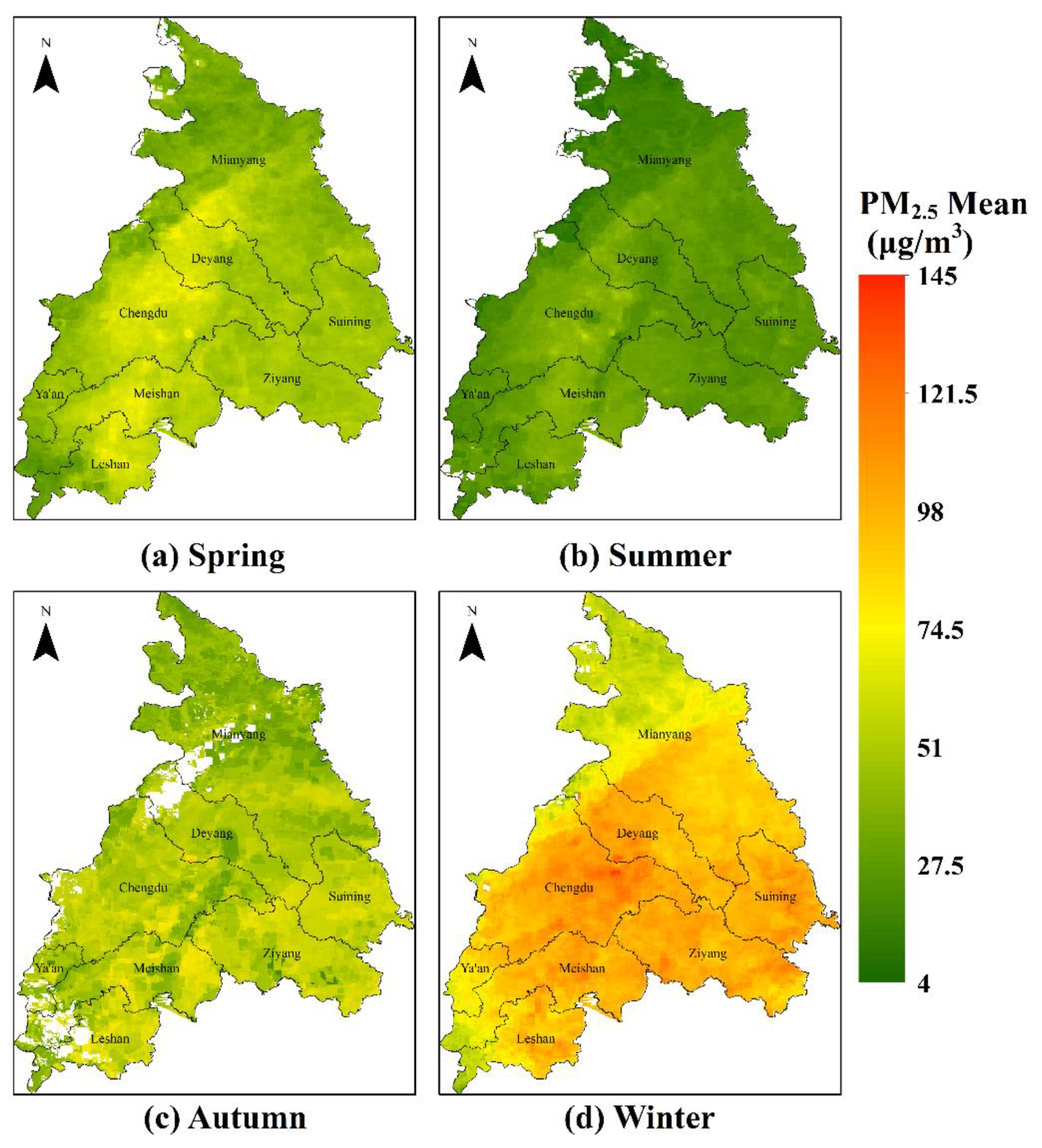
3.3. Spatiotemporal Trends of PM2.5 Concentrations

We employed the Model-I to estimate daily PM2.5 concentrations, then the maps of weekly, monthly, seasonal, and annual mean PM2.5 can be created, which are vital for the prevent and control of air pollution for local government or travel and life of city residents. As discussed before, there are a total of 129 model-valid days that have daily PM2.5 estimates during the entire study period. Figure 5a illustrates the spatial distribution of PM2.5 average from all the model-valid days at 1 km resolution for the entire study area (i.e., urban agglomeration of Chengdu Plain). It can be observed that the PM2.5 levels have obvious spatial change pattern across the study area: High PM2.5 levels are mainly located in the middle and southern areas, which are the mountain valleys of Longquan Mountains and Qionglai Mountians (Figure 5a); while low PM2.5 levels appear in rural and mountainous areas in the northwest and southwest areas. Such spatial patterns correspond well with those of ground-based monitoring sites shown in Figure 1b. It is evident that the boundaries of plains and mountains also separate areas of high PM2.5 levels areas and low PM2.5 levels areas over Chengdu Plain, indicating that the terrain has significant impact on the distribution of pollution.
The PM2.5 average is 56.86 μg/m3 during the whole study period, which is comparable to 53.86 μg/m3 of all the monitoring sites, 1.5 times more than China NAAQS of 35.0 μg/m3 for the daily mean PM2.5. The city-specific mean PM2.5 was the average of all PM2.5 grid cells that belong to one specific city, varying from 49.78 μg/m3 for Ya’an to 62.12 μg/m3 for Chengdu. The PM2.5 estimates indicate that almost the majority of people living in the study area are exposed to risky PM2.5 pollution levels, especially Chengdu, the provincial capital of Sichuan Province, with much dense population, which is a serious public concern for local government and common people. Figure 5a indicates that high PM2.5 level areas are located at areas with high-level urbanization in Chegndu Plain. Figure 5a also indicates that higher PM2.5 levels are located at main traffic roads, and several atmospheric pollution hotspots exist at a traffic hub with high density of roads in Chengdu, indicating that traffic vehicles are an important source of PM2.5, also high PM2.5 levels in urban center of Suining, Meishan, Ziyang, and Leshan.
Moreover, the seasonal mean PM2.5 estimates in the whole study area are 49.80, 30.16, 48.61, and 88.45 μg/m3 for spring (March, April, and May), summer (June, July, and August), autumn (September, October, and November), and winter (December, January, and February), respectively. From Figure 6a–d, it is easily observed that the PM2.5 levels has a remarkable seasonal variability, with the highest PM2.5 level during the winter and the lowest during the summer. The high PM2.5 concentrations during the winter are possibly caused by enhanced anthropogenic emissions from fossil fuel combustion and biomass burning, as well as unfavorable meteorological conditions such as temperature inversion during the cold periods or lower mixing height for atmospheric pollutants dispersion; the low PM2.5 concentrations during the summer are possibly due to reduced anthropogenic emissions, high humidity, and more rainfall, which is helpful for depositions of aerosol particles.

4. Discussion

In our study, we established and compared several daily ground-level PM2.5 estimation models using different PM2.5 datasets, AOT datasets, and other auxiliary variables. The results show that both model fitting and CV for all models can generate higher R2 (Table 1). Among the models, the Model-I has the best performance and agreement between satellite estimated and ground-based measured PM2.5, with model-valid days of 129 and PM2.5–AOT pairs of 1635. Compared to linear regression model performance based on the same modeling data (see Supplementary: Figure S2), the performance of Model-I is hugely improved when considering daily variations of PM2.5–AOT relationship. Model-CV results show models have over-fitting due to R2 decrease, RMSPE, and MPE increase. Model-I/Model-V has slightly better performance than Model-II/Model-VI shown in Table 1. For models fitted with only one satellite observation (Terra or Aqua), Model-III (Terra AOT, morning) is inferior to Model-IV (Aqua AOT, afternoon), with higher RMSPE and MPE, and lower R2. Besides, after estimating the missing AOT data, the number of PM2.5–AOT pairs was significantly increased from 529 to 1635, and also improved spatial and temporal coverage of PM2.5 estimates, only causing a slight degradation of performance. Thus, the process of estimating of the missing AOT is important and necessary for the study area with serious data missing.
The air pollution strongly depends on thermodynamic state of the atmosphere. The turbulence occurring in the boundary layer of the atmosphere influences the meteorological conditions, and especially the convection process and temperature inversion. It strongly influences the formation and intensity of diffusion in the atmosphere and, as a consequence, the concentration of primary and secondary atmospheric pollutants in the lower troposphere. For one day, after sunrise, the radiation increases, and the mixing layer height increases rapidly under the impact of thermal buoyancy lift, reaching the maximum at about midday. Meanwhile, the atmospheric pollutants emitted at ground will be lifted aloft along with mixing layer height rising. After noon, the mixing layer height decreases as a consequence of the reduction of convective activity driven by the heating of the Earth’ surface by sunlight and the corresponding nocturnal radiative cooling of the ground. Atmospheric pollutants (e.g., particles) confined within the mixing layer will descend to the ground due to inactive of thermodynamic state and gravitational force. Hence, the concentration of atmosphere particles increases [66].
Satellite-derived AOT represents the amount of aerosol in the whole vertical column of atmosphere from the ground to satellite altitude (not only limited to the vertical column segment close to the ground-based monitoring sites). According to the varying pattern of the atmospheric pollutants in one day described above, the PM2.5 24-h average captures more of the aerosols subsiding down to ground level at monitoring sites than does the PM2.5 time average of 10:00 and 14:00. This might explain why the Model I/V performs a little better than the Model II/VI.
As described above, the atmospheric pollutants are confined within the mixing layer, and lifted to the atmosphere. The atmospheric pollutants during satellite Aqua overpass are more uniformly mixed within the mixing layer than those during satellite Terra overpass, so the correlation between PM2.5 and AOT is much stronger, which is likely to interpret that performance of Model-IV using MAIAC Aqua AOT is better than Model-III using MAIAC Terra AOT.
In our study, the Model-I gained higher model fitting R2 of 0.81 and CV R2 of 0.77 than previous studies, e.g., the GWR model applied to the whole China mainland with overall CV R2 of 0.64 [30], to PRD area with R2 of 0.74 [33]; VIIRS night light data incorporated and applied to BTH region with R2 of 0.75 [67]; an improved model applied to three megalopolises with high pollution in China, namely, to the BTH with R2 of 0.77, to the YRD region with R2 of 0.80, and to the PRD region with R2 of 0.80 [43]; the observation-based method considered the effect of the main aerosol particle characteristics applied to BTH region, YRD, and PRD, with R2 of 0.70 (N = 331), 0.77 (N = 279), and 0.83 (N = 329) [47]; the LMEM models using only MODIS AOT at 3 km spatial resolution were applied to Beijing with R2 of 0.796 and 0.81 [44,45]. The similar models were applied in US with MAIAC AOT, e.g., applied to southeastern US with model fitting R2 of 0.83 and CV R2 of 0.67 [35], long-term (10 years) analysis with model fitting R2 of 0.71–0.85 and CV R2 of 0.62–0.78 [36] and also in northeastern US with CV R2 of 0.89 [68]. The RMSPE of Model-I CV was 17.04 μg/m3, which was higher than than in the US (<9.0 μg/m3) [21,29,34,35,36,37,38], but comparable to Beijing area with a coarser 3 km spatial resolution of PM2.5 estimates by Li (16.04 μg/m3) [44] and Xie (17.85 μg/m3) [45] but with higher R2, possibly due to the smoothing effect of satellite data with coarser resolution, representing more coverage condition of air quality. The higher RMSPE in our study area or other Chinese areas than the US was more likely due to much higher PM2.5 levels, ranging from 6.0 to 224.83 μg/m3 with the average of 59.33 μg/m3, which was up to several times as that in the United States.
Although the satellite-derived PM2.5 can provide larger spatial coverage than ground-based monitoring sites, the satellite has less temporal coverage due to its observation limitations, e.g., clouds, fogginess, surface conditions, and other factors. In our study, there are a total of 129 model-valid days, which is only about 35% for one year. In addition, due to cloudy or foggy weather in Chengdu Plain causing low sampling frequency of available satellite observations, the larger variations in the PM2.5 levels were possibly be neglected. Satellite-derived AOT should be used carefully when estimating ground-level PM2.5 concentrations in Chengdu Plain due to the data missing in heavy pollution conditions where the AOT retrieval algorithm is not valid. As air pollution has become an increasing concern for the public and government, the ground-based monitoring sites will be set up more and more, and further studies should be conducted by considering other factors affecting the PM2.5–AOT relationship.
Overall, the model-estimated PM2.5 concentrations have a good consistency with that of ground- based measurements. However, there are days and sites with large residuals as seen in Figure 3. We tried to get more accurate PM2.5 estimation at every place and every day, but there are many factors that impact the spatial variability of PM2.5-AOT relationship; in particular, mixing height, PM2.5 composition, temperature, and humidity [50,51]. Another reason is the number of ground monitoring PM2.5 sites and its uneven spatial location.

5. Conclusions

In this study, we developed an improved linear mixed effects model (LMEM) to estimate the daily ground-level PM2.5 concentrations referring to atmospheric particulate matter with a diameter of less than 2.5 μm by incorporating humidity and gridded population data. It is should be noted that to reduce the uncertainty caused by inconsistency of spatiotemporal between aerosol optical thickness (AOT) and meteorological data, both of them should be generated from the same satellite.
The model is implemented to the urban agglomeration of Chengdu Plain, where heavy atmospheric particle pollution is common and frequent. The results indicate that the PM2.5–AOT relationship was significantly improved when considering the day-to-day variability, with a much higher accuracy than simple linear regression (see Supplementary: Figure S3) with R2 of 0.81 versus 0.49, lower root mean squared prediction error (RMSPE) of 15.47 μg/m3 versus 25.32 μg/m3, mean prediction error (MPE) of 11.09 μg/m3 versus 18.87 μg/m3; the mean PM2.5 estimates across the whole study area was 56.86 μg/m3, which is comparable to 53.86 μg/m3 of all the monitoring sites, indicating good consistency of PM2.5 estimates and ground monitoring sites.
The results demonstrate that the PM2.5 levels in the study area have an obvious spatial pattern, with high PM2.5 levels mainly located in middle and southern areas, and low PM2.5 levels in rural and mountainous areas. The PM2.5 levels also have a remarkable seasonal variability, with the highest level during the winter and the lowest during the summer.
Besides, the product of daily PM2.5 estimation at 1 km spatial resolution in heavily polluted areas with high accuracy are valuable for local government pollution monitoring, public health research, and urban air quality control.

Supplementary Materials

The following are available online at https://www.mdpi.com/2073-4433/10/5/245/s1, Figure S1: Scatterplots of MAIAC AOT versus AERONET, Figure S2: Scatterplots of daily PM2.5 versus daily AOT, Figure S3: Scatterplots of Estimated PM2.5 versus Measured PM2.5, Table S1: Geolocation of 36 Monitoring Sites in Urban Agglomeration of Chengdu Plain, Table S2: Statistical Summary of Daily PM2.5 24-h Average for Each Site in Urban Agglomeration of Chengdu Plain, Table S3: Statistical Summary of Daily PM2.5 time average of 10 a.m. and 2 p.m. for Each Site in Urban Agglomeration of Chengdu Plain, Table S4: Statistical Summary of Daily AOT Average for Each Site in Urban Agglomeration of Chengdu Plain.

Author Contributions

W.H., conceived and designed the experiments; W.H. and L.T. analyzed the data; W.H. wrote the original draft of the paper, which was revised by L.T.

Funding

This research was funded by the National Natural Science Foundation of China (Grant No. 41771433) and Advanced Research Project (Grant No. 30102060301).

Acknowledgments

The authors would like to thank the MAIAC algorithm team for offering AOT data, SEDAC team for offering GPWv4 data.

Conflicts of Interest

The authors declare no conflict of interest.

Appendix A

Table A1. The acronyms and definitions used in this article area displayed below table.
AcronymsDefinition
AERONETAerosol Robotic Network
AOTAerosol Optical Thickness
AVHRRAdvanced Very High Resolution Radiometer
BRDFBidirectional Reflectance Distribution Function
BTHBeijing-Tianjin-Hebei
CVCross-Validation
CWVColumn Water Vapor
GAMGeneralized Additive Model
GPWGridded Population of the World
GPWv4GPW collection in fourth version
GWRGeographically Weighted Regression
LMEMLinear Mixed Effect Model
LURLand Use Regression
MAIACMulti-Angle Implementation of Atmospheric Correction
MAIAC AOTAOT products produced with MAIAC algorithm
MAIAC CWVCWV products produced with MAIAC algorithm
MAIAC-Aqua AOTAOT products produced with Aqua satellite using MAIAC algorithm
MAIAC-Terra AOTAOT products produced with Terra satellite using MAIAC algorithm
MISRMulti-angle Imaging SpectroRadiometer
MOD04MODIS Aerosol Product with 10 km resolution
MODISMODerate resolution Imaging Spectroradiometer
MPEMean Prediction Error
China NAAQSChina National Ambient Air Quality Standard
NASANational Aeronautics and Space Administration
PM2.5Particulates with aerodynamic diameters of less than 2.5 μm
POPPopulation data
PRDPearl River Delta
RMSPERoot Mean Squared Prediction Error
SeaWiFSSea-Viewing Wide Field-of-View Sensor
SEDACSocioeconomic Data and Application Center
SRSurface Reflectance
SRCSpectral Regression Coefficient
TEOMTapered Element Oscillating Microbalance
TOMSTotal Ozone Mapping Spectrometer
VIIRSVisible Infrared Imaging Radiometer Suite
WHOWorld Health Organization
YRDYangtze River Delta

References

  1. Lu, F.; Xu, D.; Cheng, Y.; Dong, S.; Guo, C.; Jiang, X.; Zheng, X. Systematic review and meta-analysis of the adverse health effects of ambient PM2.5 and PM10 pollution in the Chinese population. Environ. Res. 2015, 136, 196–204. [Google Scholar] [CrossRef] [PubMed]
  2. Tian, Y.; Xiang, X.; Wu, Y.; Cao, Y.; Song, J.; Sun, K.; Liu, H.; Hu, Y. Fine Particulate Air Pollution and First Hospital Admissions for Ischemic Stroke in Beijing, China. Sci. Rep. 2017, 7, 3897. [Google Scholar] [CrossRef]
  3. Weichenthal, S.; Villeneuve, P.J.; Burnett, R.T.; van Donkelaar, A.; Martin, R.V.; Jones, R.R.; DellaValle, C.T.; Sandler, D.P.; Ward, M.H.; Hoppin, J.A. Long-term exposure to fine particulate matter: Association with nonaccidental and cardiovascular mortality in the agricultural health study cohort. Environ. Health Perspect. 2014, 122, 609–615. [Google Scholar] [CrossRef]
  4. Brook, R.D.; Cakmak, S.; Turner, M.C.; Brook, J.R.; Crouse, D.L.; Peters, P.A.; van Donkelaar, A.; Villeneuve, P.J.; Brion, O.; Jerrett, M.; et al. Long-term fine particulate matter exposure and mortality from diabetes in Canada. Diabetes Care 2013, 36, 3313–3320. [Google Scholar] [CrossRef]
  5. Crouse, D.L.; Peters, P.A.; van Donkelaar, A.; Goldberg, M.S.; Villeneuve, P.J.; Brion, O.; Khan, S.; Atari, D.O.; Jerrett, M.; Pope, C.A.; et al. Risk of nonaccidental and cardiovascular mortality in relation to long-term exposure to low concentrations of fine particulate matter: A Canadian national-level cohort study. Environ. Health Perspect. 2012, 120, 708–714. [Google Scholar] [CrossRef]
  6. Dockery, D.W.; Schwartz, J. Particulate air pollution and mortality: More than the Philadelphia story. Epidemiology 1995, 6, 629–632. [Google Scholar] [CrossRef]
  7. Moolgavkar, S.H.; Luebeck, E.G. A critical review of the evidence on particulate air pollution and mortality. Epidemiology 1996, 7, 420–428. [Google Scholar] [CrossRef] [PubMed]
  8. Ito, K.; Thurston, G.; Silverman, R. Characterization of PM2.5, gaseous pollutants, and meteorological interactions in the context of time-series health effects models. J. Expo. Sci. Environ. Epidemiol. 2008, 17 (Suppl. 2), S45–S60. [Google Scholar] [CrossRef]
  9. Lall, R.; Kendall, M.; Ito, K.; Thurston, G. Estimation of historical annual PM2.5 exposures for health effects assessment. Atmos. Environ. 2004, 38, 5217–5226. [Google Scholar] [CrossRef]
  10. Apte, J.S.; Messier, K.P.; Gani, S.; Brauer, M.; Kirchstetter, T.W.; Lunden, M.M.; Marshall, J.D.; Portier, C.J.; Rch, V.; Hamburg, S.P. High-Resolution Air Pollution Mapping with Google Street View Cars: Exploiting Big Data. Environ. Sci. Technol. 2017, 51, 6999–7008. [Google Scholar] [CrossRef] [PubMed]
  11. Hoff, R.M.; Christopher, S.A. Remote sensing of particulate pollution from space: Have we reached the promised land? Air Repair 2009, 59, 642–644. [Google Scholar] [CrossRef]
  12. Kaufman, Y.J.; Tanré, D.; Remer, L.A.; Vermote, E.F.; Chu, A.; Holben, B.N. Operational remote sensing of tropospheric aerosol over land from EOS moderate resolution imaging spectroradiometer. J. Geophys. Res. Atmos. 1997, 102, 17017–17051. [Google Scholar] [CrossRef]
  13. Kaufman, Y.J. Satellite sensing of aerosol absorption. J. Geophys. Res. 1987, 92, 4307–4317. [Google Scholar] [CrossRef]
  14. Kaufman, Y.J. Aerosol optical thickness and atmospheric path radiance. J. Geophys. Res. Atmos. 1993, 98, 2677–2692. [Google Scholar] [CrossRef]
  15. Fraser, R.S.; Kaufman, Y.J.; Mahoney, R. Satellite measurements of aerosol mass and transport. Atmos. Environ. 1984, 18, 2577–2584. [Google Scholar] [CrossRef]
  16. Li, Z.; Zhao, X.; Kahn, R.; Mishchenko, M.; Remer, L.; Lee, K.H.; Wang, M.; Laszlo, I.; Nakajima, T.; Maring, H. Uncertainties in satellite remote sensing of aerosols and impact on monitoring its long-term trend: A review and perspective. Ann. Geophys. 2009, 27, 2755–2770. [Google Scholar] [CrossRef]
  17. Laszlo, I. Aerosol Retrieval from SNPP/VIIRS: Analysis of Technique and Data Quality. In Proceedings of the EGU General Assembly 2013, Vienna, Austria, 7–12 April 2013. [Google Scholar]
  18. Engel-Cox, J.A.; Hoff, R.M.; Haymet, A.D.J. Recommendations on the Use of Satellite Remote-Sensing Data for Urban Air Quality. J. Air Waste Manag. Assoc. 2004, 54, 1360–1371. [Google Scholar] [CrossRef]
  19. Engel-Cox, J.A.; Holloman, C.H.; Coutant, B.W.; Hoff, R.M. Qualitative and quantitative evaluation of MODIS satellite sensor data for regional and urban scale air quality. Atmos. Environ. 2004, 38, 2495–2509. [Google Scholar] [CrossRef]
  20. Wang, J.; Christopher, S.A. Intercomparison between satellite-derived aerosol optical thickness and PM2. 5 mass: Implications for air quality studies. Geophys. Res. Lett. 2003, 30. [Google Scholar] [CrossRef]
  21. Liu, Y.; Sarnat, J.A.; Kilaru, V.; Jacob, D.J.; Koutrakis, P. Estimating ground-level PM2.5 in the Eastern United States using satellite remote sensing. Environ. Sci. Technol. 2005, 39, 3269–3278. [Google Scholar] [CrossRef] [PubMed]
  22. Gupta, P.; Christopher, S.A. Particulate matter air quality assessment using integrated surface, satellite, and meteorological products: Multiple regression approach. J. Geophys. Res. Atmos. 2009, 114. [Google Scholar] [CrossRef]
  23. Gupta, P.; Christopher, S.A. Particulate matter air quality assessment using integrated surface, satellite, and meteorological products: 2. A neural network approach. J. Geophys. Res. 2009, 114. [Google Scholar] [CrossRef]
  24. Liu, Y.; Paciorek, C.J.; Koutrakis, P. Estimating regional spatial and temporal variability of PM2.5 concentrations using satellite data, meteorology, and land use information. Environ. Health Perspect. 2009, 117, 886–892. [Google Scholar] [CrossRef] [PubMed]
  25. Strawa, A.W.; Chatfield, R.B.; Legg, M.; Scarnato, B.; Esswein, R. Improving retrievals of regional fine particulate matter concentrations from moderate resolution imaging spectroradiometer (MODIS) and ozone monitoring instrument (OMI) multisatellite observations. J. Air Waste Manag. Assoc. 2013, 63, 1434–1446. [Google Scholar] [CrossRef]
  26. Kloog, I.; Nordio, F.; Coull, B.A.; Schwartz, J. Incorporating local land use regression and satellite aerosol optical depth in a hybrid model of spatiotemporal PM2.5 xxposures in the Mid-Atlantic states. Environ. Sci. Technol. 2012, 46, 11913–11921. [Google Scholar] [CrossRef] [PubMed]
  27. David Knibbs, L.; van Donkelaar, A.; Martin, R.; Bechle, M.; Brauer, M.; Cohen, D.D.; Cowie, C.; Dirgawati, M.; Guo, Y.; Hanigan, I.C.; et al. Satellite-bBased land use regression for continental-scale long-term ambient PM2.5 exposure assessment in Australia. Environ. Sci. Technol. 2018, 52, 12445–12455. [Google Scholar] [CrossRef] [PubMed]
  28. Li, R.; Ma, T.; Xu, Q.; Song, X. Using MAIAC AOD to verify the PM2.5 spatial patterns of a land use regression model. Environ. Pollut. 2018, 243, 501–509. [Google Scholar] [CrossRef]
  29. Hu, X.; Waller, L.A.; Al-Hamdan, M.Z.; Crosson, W.L.; Estes, M.G., Jr.; Estes, S.M.; Quattrochi, D.A.; Sarnat, J.A.; Liu, Y. Estimating ground-level PM2.5 concentrations in the southeastern U.S. using geographically weighted regression. Environ. Res. 2013, 121, 1–10. [Google Scholar] [CrossRef]
  30. Ma, Z.; Hu, X.; Huang, L.; Bi, J.; Liu, Y. Estimating ground-level PM2.5 in China using satellite remote sensing. Environ. Sci. Technol. 2014, 48, 7436–7444. [Google Scholar] [CrossRef]
  31. van Donkelaar, A.; Martin, R.V.; Brauer, M.; Hsu, N.C.; Kahn, R.A.; Levy, R.C.; Lyapustin, A.; Sayer, A.M.; Winker, D.M. Global Estimates of Fine Particulate Matter using a Combined Geophysical-Statistical Method with Information from Satellites, Models, and Monitors. Environ. Sci. Technol. 2016, 50, 3762–3772. [Google Scholar] [CrossRef]
  32. Guo, Y.; Tang, Q.; Gong, D.-Y.; Zhang, Z. Estimating ground-level PM2.5 concentrations in Beijing using a satellite-based geographically and temporally weighted regression model. Remote Sens. Environ. 2017, 198, 140–149. [Google Scholar] [CrossRef]
  33. Song, W.; Jia, H.; Huang, J.; Zhang, Y. A satellite-based geographically weighted regression model for regional PM2.5 estimation over the Pearl River Delta region in China. Remote Sens. Environ. 2014, 154, 1–7. [Google Scholar] [CrossRef]
  34. Lee, H.J.; Liu, Y.; Coull, B.A.; Schwartz, J.; Koutrakis, P. A novel calibration approach of MODIS AOD data to predict PM2.5 concentrations. Atmos. Chem. Phys. 2011, 11, 7991–8002. [Google Scholar] [CrossRef]
  35. Hu, X.; Waller, L.A.; Lyapustin, A.; Wang, Y.; Al-Hamdan, M.Z.; Crosson, W.L.; Estes, M.G.; Estes, S.M.; Quattrochi, D.A.; Puttaswamy, S.J.; et al. Estimating ground-level PM2.5 concentrations in the Southeastern United States using MAIAC AOD retrievals and a two-stage model. Remote Sens. Environ. 2014, 140, 220–232. [Google Scholar] [CrossRef]
  36. Hu, X.; Waller, L.A.; Lyapustin, A.; Wang, Y.; Liu, Y. 10-year spatial and temporal trends of PM2.5 concentrations in the southeastern US estimated using high-resolution satellite data. Atmos. Chem. Phys. 2014, 14, 6301–6314. [Google Scholar] [CrossRef] [PubMed]
  37. Hu, X.; Waller, L.A.; Lyapustin, A.; Wang, Y.; Liu, Y. Improving satellite-driven PM2.5 models with Moderate Resolution Imaging Spectroradiometer fire counts in the southeastern U.S. J. Geophys. Res. Atmos. 2014, 119, 375–386. [Google Scholar] [CrossRef] [PubMed]
  38. Lee, H.J.; Chatfield, R.B.; Strawa, A.W. Enhancing the applicability of satellite remote sensing for PM2.5 estimation using MODIS deep blue AOD and land use regression in California, United States. Environ. Sci. Technol. 2016, 50, 6546–6555. [Google Scholar] [CrossRef] [PubMed]
  39. Ma, Z.; Hu, X.; Sayer, A.M.; Levy, R.; Zhang, Q.; Xue, Y.; Tong, S.; Bi, J.; Huang, L.; Liu, Y. Satellite-bsed spatiotemporal trends in PM2.5 concentrations: China, 2004–2013. Environ. Health Perspect. 2016, 124, 184–192. [Google Scholar] [CrossRef]
  40. Ma, Z.; Liu, Y.; Zhao, Q.; Liu, M.; Zhou, Y.; Bi, J. Satellite-derived high resolution PM2.5 concentrations in Yangtze River Delta Region of China using improved linear mixed effects model. Atmos. Environ. 2016, 133, 156–164. [Google Scholar] [CrossRef]
  41. Schliep, E.M.; Gelfand, A.E.; Holland, D.M. Autoregressive spatially varying coefficients model for predicting daily PM2.5 using VIIRS satellite AOT. Adv. Stat. Clim. Meteorol. Oceanogr. 2015, 1, 59–74. [Google Scholar] [CrossRef]
  42. Zhang, X.; Hu, H. Improving satellite-driven PM2.5 models with VIIRS nighttime light data in the Beijing–Tianjin–Hebei region, China. Remote Sens. 2017, 9, 908. [Google Scholar] [CrossRef]
  43. Zheng, Y.; Zhang, Q.; Liu, Y.; Geng, G.; He, K. Estimating ground-level PM2.5 concentrations over three megalopolises in China using satellite-derived aerosol optical depth measurements. Atmos. Environ. 2016, 124, 232–242. [Google Scholar] [CrossRef]
  44. Li, R. Estimating ground-level PM2.5 using fine-resolution satellite data in the megacity of Beijing, China. Aerosol Air Qual. Res. 2015, 15, 1347–1356. [Google Scholar] [CrossRef]
  45. Xie, Y.; Wang, Y.; Zhang, K.; Dong, W.; Lv, B.; Bai, Y. Daily estimation of ground-level PM2.5 concentrations over Beijing using 3 km resolution MODIS AOD. Environ. Sci. Technol. 2015, 49, 12280–12288. [Google Scholar] [CrossRef] [PubMed]
  46. Lee, A.K.Y.; Ling, T.Y.; Chan, C.K. Understanding hygroscopic growth and phase transformation of aerosols using single particle Raman spectroscopy in an electrodynamic balance. Faraday Discuss. 2008, 137, 245. [Google Scholar] [CrossRef]
  47. Lin, C.; Li, Y.; Yuan, Z.; Lau, A.K.H.; Li, C.; Fung, J.C.H. Using satellite remote sensing data to estimate the high-resolution distribution of ground-level PM2.5. Remote Sens. Environ. 2015, 156, 117–128. [Google Scholar] [CrossRef]
  48. Wang, Z.; Chen, L.; Tao, J.; Liu, Y.; Hu, X.; Tao, M. An empirical method of RH correction for satellite estimation of ground-level PM concentrations. Atmos. Environ. 2014, 95, 71–81. [Google Scholar] [CrossRef]
  49. Wang, Z.; Chen, L.; Tao, J.; Zhang, Y.; Su, L. Satellite-based estimation of regional particulate matter (PM) in Beijing using vertical-and-RH correcting method. Remote Sens. Environ. 2010, 114, 50–63. [Google Scholar] [CrossRef]
  50. Chudnovsky, A.; Tang, C.-H.; Lyapustin, A.; Wang, Y.; Schwartz, J.; Koutrakis, P. A critical assessment of high resolution aerosol optical depth (AOD) retrievals for fine particulate matter (PM) predictions. Atmos. Chem. Phys. 2013, 13, 10907–10917. [Google Scholar] [CrossRef]
  51. Chudnovsky, A.A.; Kostinski, A.; Lyapustin, A.; Koutrakis, P. Spatial scales of pollution from variable resolution satellite imaging. Environ. Pollut. 2013, 172, 131–138. [Google Scholar] [CrossRef]
  52. Lyapustin, A.; Martonchik, J.; Wang, Y.; Laszlo, I.; Korkin, S. Multiangle implementation of atmospheric correction (MAIAC): 1. Radiative transfer basis and look-up tables. J. Geophys. Res. 2011, 116. [Google Scholar] [CrossRef]
  53. Lyapustin, A.; Wang, Y.; Laszlo, I.; Kahn, R.; Korkin, S.; Remer, L.; Levy, R.; Reid, J.S. Multiangle implementation of atmospheric correction (MAIAC): 2. Aerosol algorithm. J. Geophys. Res. 2011, 116. [Google Scholar] [CrossRef]
  54. Lowsen, D.H.; Conway, G.A. Air Pollution in Major Chinese Cities: Some Progress, But Much More to Do. J. Environ. Prot. 2016, 7, 2081–2094. [Google Scholar] [CrossRef]
  55. Liao, T.; Wang, S.; Ai, J.; Gui, K.; Duan, B.; Zhao, Q.; Zhang, X.; Jiang, W.; Sun, Y. Heavy pollution episodes, transport pathways and potential sources of PM2.5 during the winter of 2013 in Chengdu (China). Sci. Total Environ. 2017, 584–585, 1056–1065. [Google Scholar] [CrossRef] [PubMed]
  56. Qiao, X.; Jaffe, D.; Tang, Y.; Bresnahan, M.; Song, J. Evaluation of air quality in Chengdu, Sichuan Basin, China: Are China’s air quality standards sufficient yet? Environ. Monit. Assess. 2015, 187, 250. [Google Scholar] [CrossRef]
  57. Fan, L.U. Design of Real-time Ambient Particulate Monitoring System Based on TEOM Technology. J. Atmos. Environ. Opt. 2007, 2, 361–365. [Google Scholar]
  58. Ministry of Ecology and Environment. Determination of Atmospheric Articles PM10 and PM2.5 in Ambient Air by Gravimetric Method. Available online: http://english.mee.gov.cn/Resources/standards/Air_Environment/air_method/201111/t20111101_219390.shtml (accessed on 27 December 2018).
  59. Koelemeijer, R.; Homan, C.; Matthijsen, J. Comparison of spatial and temporal variations of aerosol optical thickness and particulate matter over Europe. Atmos. Environ. 2006, 40, 5304–5315. [Google Scholar] [CrossRef]
  60. NASA Center for Climate Simulation. MAIAC AOT Data Repository. Available online: https://portal.nccs.nasa.gov/datashare/maiac/DataRelease/ (accessed on 27 December 2018).
  61. Holben, B.N.; Eck, T.F.; Slutsker, I.; Tanré, D.; Buis, J.P.; Setzer, A.; Vermote, E.; Reagan, J.A.; Kaufman, Y.J.; Nakajima, T. AERONET—A Federated Instrument Network and Data Archive for Aerosol Characterization. Remote Sens. Environ. 1998, 66, 1–16. [Google Scholar] [CrossRef]
  62. Instesre. Calculating the Angstrom Turbidity Coefficient and Other Quantities Related to Aerosol Optical Thickness. Available online: http://www.instesre.org/Aerosols/angstrom.htm (accessed on 29 March 2019).
  63. Ångström, A. The parameters of atmospheric turbidity. Tellus 1963, 16, 64–75. [Google Scholar] [CrossRef]
  64. Socioeconomic Data and Applications Center. Gridded Population of the World (GPW), v4. Available online: http://sedac.ciesin.columbia.edu/data/collection/gpw-v4 (accessed on 27 December 2018).
  65. Kohavi, R. A Study of Cross-Validation and Bootstrap for Accuracy Estimation and Model Selection. In Proceedings of the 4th International Joint Conference on Artificial Intelligence, Montreal, QC, Canada, 20–25 August 1995; Volume 14. [Google Scholar]
  66. Tang, G.; Zhu, X.; Hu, B.; Xin, J.; Wang, L.; Münkel, C.; Mao, G.; Wang, Y. Impact of emission controls on air quality in Beijing during APEC 2014: Lidar ceilometer observations. Atmos. Chem. Phys. 2015, 15, 12667–12680. [Google Scholar] [CrossRef]
  67. Wei, W.; Zengxin, P.; Feiyue, M.; Wei, G.; Shenghui, F.; Lin, D. Deriving Hourly PM2.5 Concentrations from Himawari-8 AODs over Beijing-Tianjin-Hebei in China. Remote Sens. 2017, 9, 858. [Google Scholar] [CrossRef]
  68. Chudnovsky, A.A.; Koutrakis, P.; Kloog, I.; Melly, S.; Nordio, F.; Lyapustin, A.; Wang, Y.; Schwartz, J. Fine particulate matter predictions using high resolution Aerosol Optical Depth (AOD) retrievals. Atmos. Environ. 2014, 89, 189–198. [Google Scholar] [CrossRef]
Figure 1. (a) Study area location at China (displayed with red polygon in the map); (b) satellite map shows that study area (red lines) is surrounded by mountains in the west, north, and northeast (Satellite imagery source: Esri, DigitalGlobe, GeoEye); (c) annual average PM2.5 24-h average (μg/m3) for each site, which is classified into six levels represented by different color; (d) the spatial distribution of average of multi-angle implementation of atmospheric correction (MAIAC) aerosol optical thickness (AOT) at 1 km resolution during 2015. The boundaries of eight province-controlled cities are shown in black lines.
Atmosphere 10 00245 g001
Figure 2. Boxplots statistics of estimation performance at all the 36 sites for R2, intercept, slope, root mean squared prediction error (RMSPE) (μg/m3), MPE (μg/m3). (a) Model fitting; (b) model validation. ‘I’ denotes models using PM2.5 24-h average, and ‘II’ denotes models using PM2.5 time average of 10:00 and 14:00.
Atmosphere 10 00245 g002
Figure 3. Scatterplots for model fitting and cross validation between estimated and measured PM2.5 for each year. (a) Model fitting; (b) model cross validation. The red solid line represents the regression line and the green dashed line is the 1:1 line with slope of 1.0; ‘I’ denotes models using PM2.5 24-h average, and ‘II’ denotes models using PM2.5 time average of 10:00 and 14:00.
Atmosphere 10 00245 g003
Figure 4. The differences between estimated and measured PM2.5 (μg/m3) at each monitoring site during 2015.
Atmosphere 10 00245 g004
Figure 5. (a) Maps of mean PM2.5 concentration (μg/m3) averaged from all PM2.5 estimates model valid days for 2015, and the back ground is traffic map. (b) Satellite imagery map for Chengdu Plain (Satellite imagery source: Esri, DigitalGlobe, GeoEye).
Atmosphere 10 00245 g005
Figure 6. Maps of seasonal mean PM2.5 concentration (μg/m3) calculated with daily estimation for the year of 2015. (a) Spring, (b) summer, (c) autumn, (d) winter. The white blank areas indicate missing value due to lack of MAIAC AOT data. The boundaries of eight cities area shown in black lines.
Atmosphere 10 00245 g006
Table 1. Model performance summary.
ModelN 1M 2Model FittingCross Validation
R2RMSPE (μg/m3)MPE (μg/m3)R2RMSPE (μg/m3)MPE (μg/m3)
Model-I 312916350.8115.4711.090.7717.0412.31
Model-II 412916350.7819.9614.090.7421.7815.53
Model-III 511013460.6527.0319.570.5829.3321.42
Model-IV 6807620.8517.8411.900.8020.1813.64
Model-V 7535290.8614.6210.560.8216.5612.11
Model-VI 8535290.8219.7613.850.7822.1215.63
1 Denotes the number of days used in model fitting. 2 Denotes the number of PM2.5-AOT pairs used in model fitting. 3 Denotes models using PM25 24-h average and AOT average of adjusted Terra and Aqua MAIAC AOT. 4 Denotes models using PM2.5 average between 10:00 and14:00, and AOT average of adjusted Terra and Aqua MAIAC AOT. 5 Denotes models using Terra MAIAC AOT and average between 10:00 and 11:00. 6 Denotes models using Aqua MAIAC AOT and PM2.5 average between 13:00 and 14:00. 7 Denotes models using PM25 24-h average and AOT average of Terra and Aqua MAIAC AOT. 8 Denotes models using PM2.5 average between 10:00 and 14:00, and AOT average of Terra and Aqua.

