Optimised Heat Pump Management for Increasing Photovoltaic Penetration into the Electricity Grid

 , , , and
Abstract

1. Introduction
2. Methodology and Simulation Framework
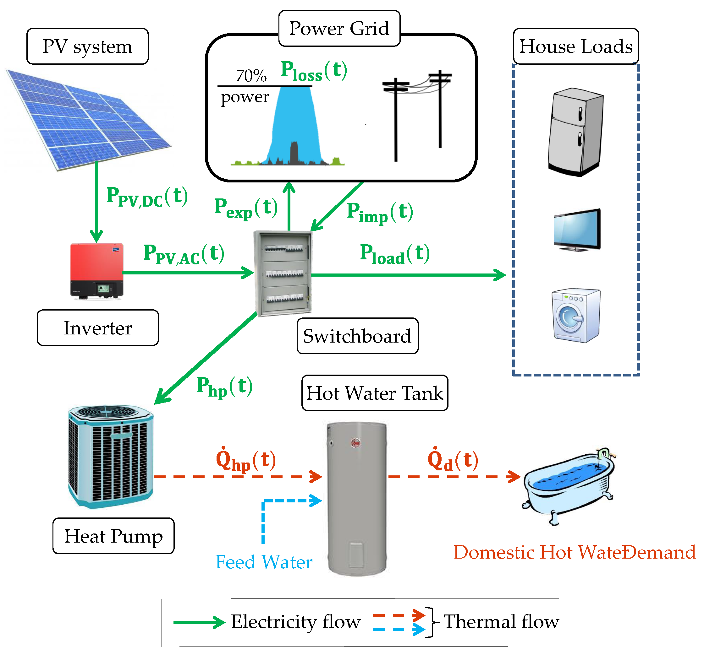
2.1. System Components and Modelling
2.1.1. Inverter
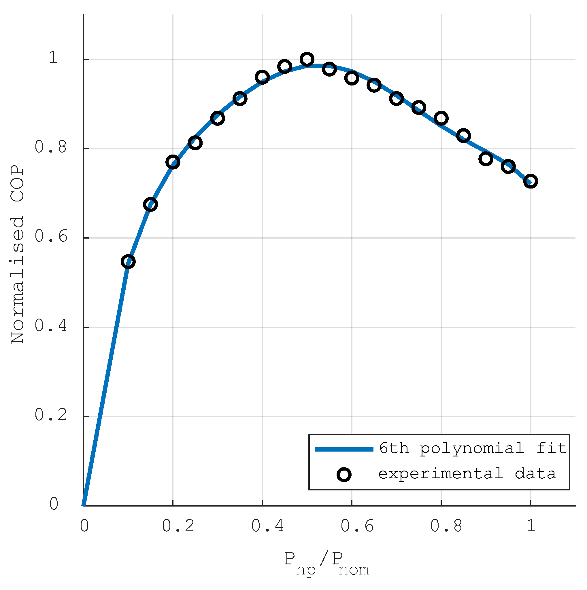
2.1.2. Heat Pump
2.1.3. Domestic Hot Water Tank
2.2. HP Operation Optimisation
2.2.1. Data Input
2.2.2. Parameters of Optimal Control Problem
2.2.3. Nonlinear Optimisation Problem
2.2.4. Mixed-Integer Linear Optimisation Problem
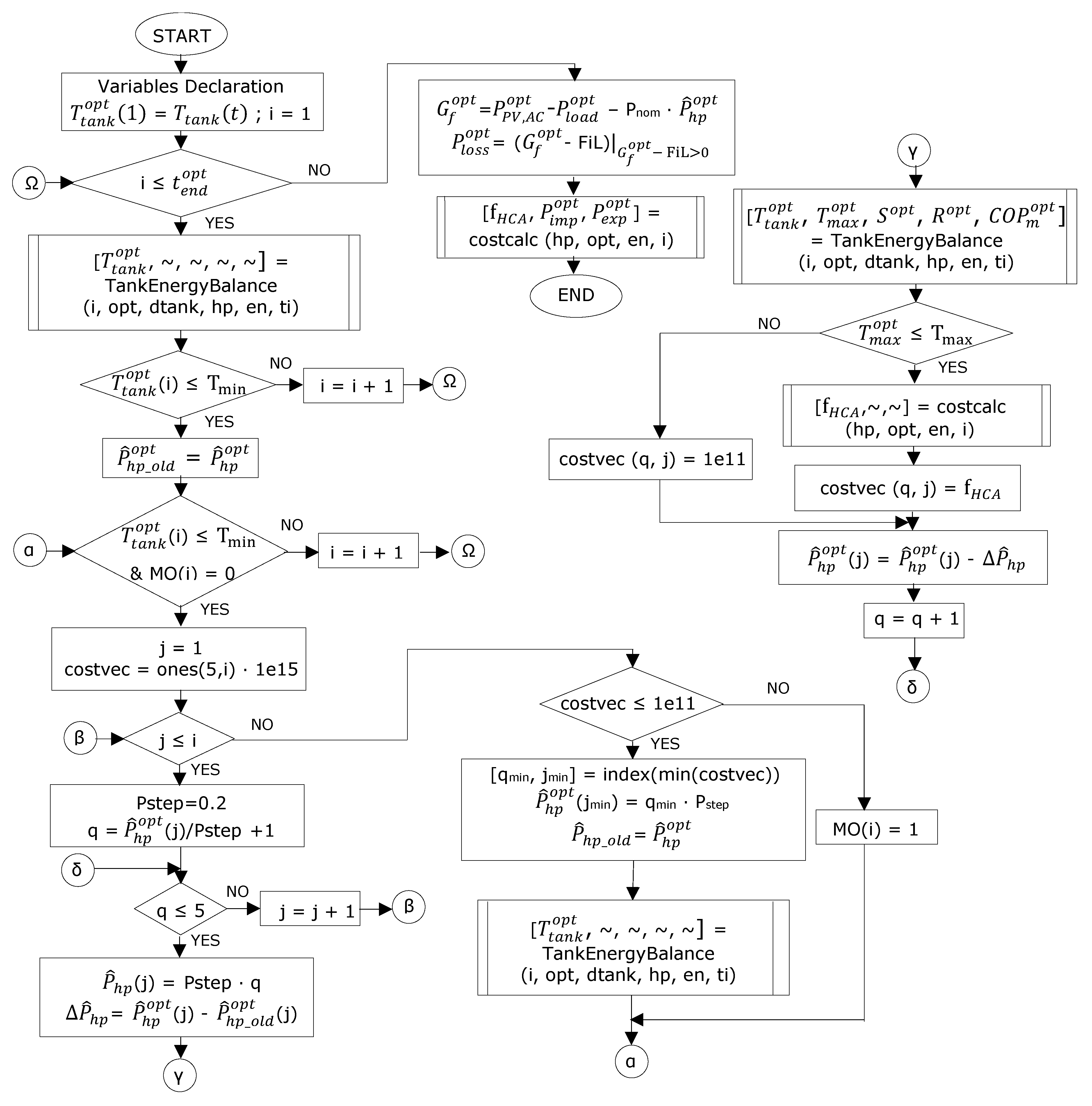
2.2.5. Heuristic Optimal Control Problem
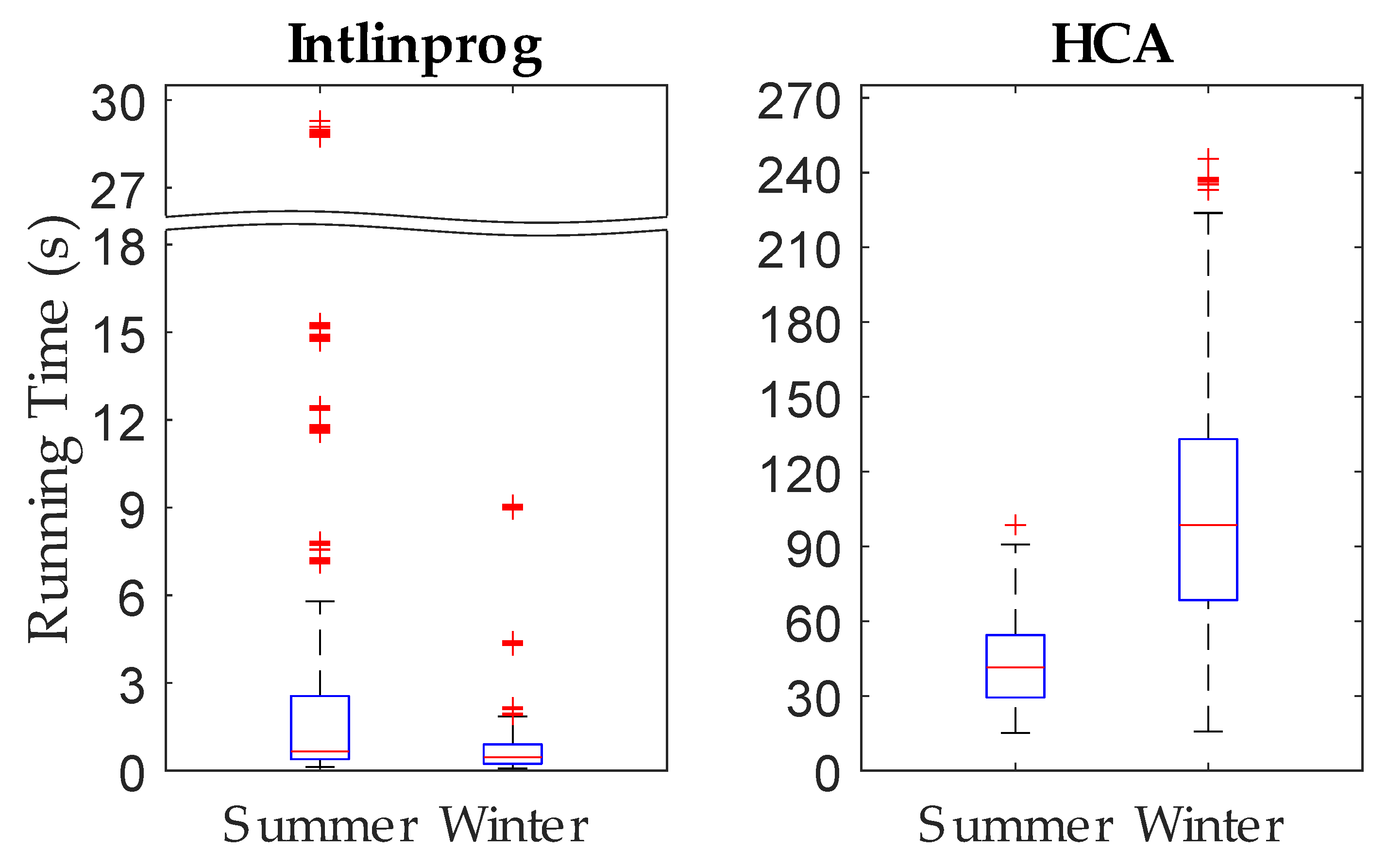
2.2.6. Optimisation Solvers
2.2.7. Instantaneous Control Algorithm (ICA)
2.3. Evaluation Metrics
3. Results and Discussion
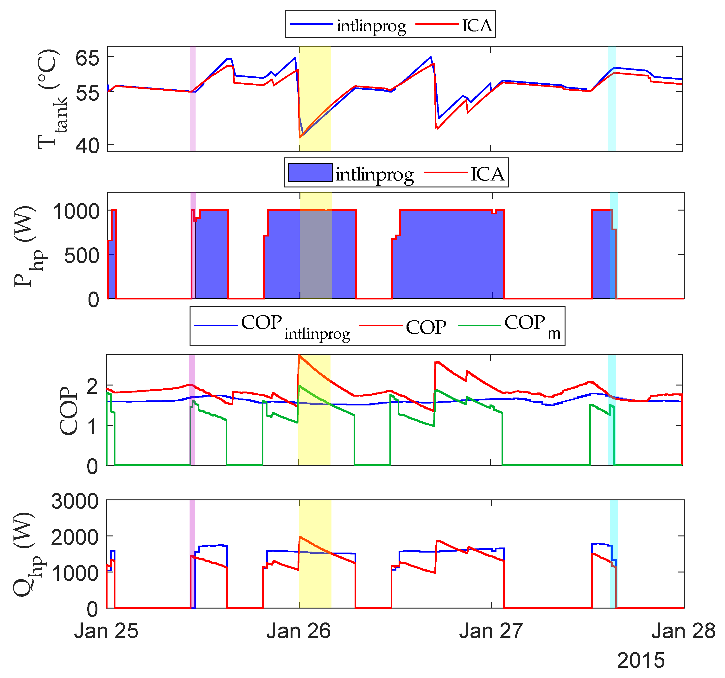
3.1. Short-Term Simulations
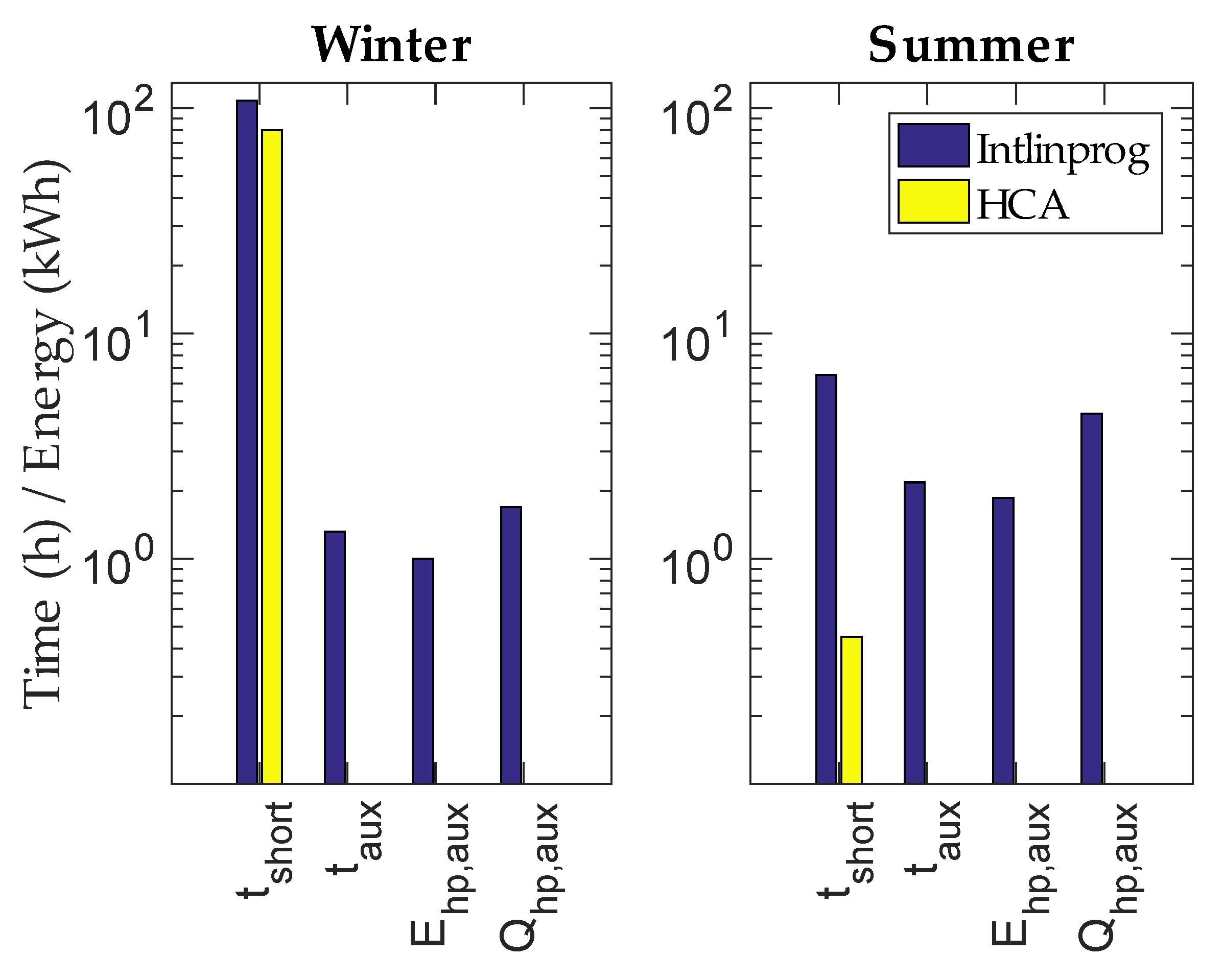
3.2. Long-Term Simulations
4. Conclusions
Author Contributions
Funding
Acknowledgments
Conflicts of Interest
Abbreviations
| AWHP | Air-to-Water Source Heat Pump |
| CAPEX | Capital Expenditures |
| COP | Coefficient of Performance |
| DHW | Domestic Hot Water |
| FiL | Feed-in Power Limit |
| FiT | Feed-in Tariff |
| HCA | Heuristic Control Algorithm |
| HP | Heat Pump |
| ICA | Instantaneous Control Algorithm |
| MILP | Mixed Integer Linear Programming |
| NLP | Nonlinear Programming |
| LP | Linear Programming |
| OCP | Optimal Control Problem |
| OPEX | Operating Expenditures |
| PLR | Part-Load Ratio |
| PV | Photovoltaics |
| RBC | Rule-Based Control |
| RE | Renewable Energy |
| TES | Thermal Energy Storage |
Appendix A

| Pos | Property | Unit | Description | Value |
|---|---|---|---|---|
| DHW Tank (dtank) | ||||
| Inverter (inv) | ||||
| Environment (en) | ||||
| 1 | W | Photovoltaic DC-production | ||
| 2 | W | Household electric consumption profile | ||
| Temps (ti) | ||||
| 3 | min | Starting time of simulation | [1, 525,601] | |
| 4 | min | End of simulation time | [1, 525,601] | |
| 5 | min | Simulation time step | 1 | |
| Heat Pump (hp) | ||||
| 6 | Unitless | Independent coefficient | 5.5930 | |
| 7 | 1/°C | -dependent coefficient | 0.0569 | |
| 8 | 1/°C | -dependent coefficient | −0.0661 | |
| 9 | Unitless | 1st order part-load efficiency coefficient | 8.3350 | |
| 10 | Unitless | 2nd order part-load efficiency coefficient | −38.0747 | |
| 11 | Unitless | 3rd order part-load efficiency coefficient | 104.6758 | |
| 12 | Unitless | 4th order part-load efficiency coefficient | −159.6927 | |
| 13 | Unitless | 5th order part-load efficiency coefficient | 121.4477 | |
| 14 | Unitless | 6th order part-load efficiency coefficient | −35.9697 | |
| Instantaneous Control Algorithm (ins) | ||||
| 15 | Unitless | Heat pump coefficient of performance | ||
| 16 | W | Exporting grid flux | ||
| 17 | W | Heat pump electric power | ||
| 18 | W | Importing grid flux | ||
| 19 | W | Household electricity consumption | ||
| 20 | W | Power curtailment due to | ||
| 21 | W | Photovoltaic-AC production | ||
| 22 | °C | Maximum heat pump supply temperature | 65 | |
| 23 | °C | Minimum tank temperature | 55 | |
| Optimisation (opt) | ||||
| 24 | Unitless | Optimised heat pump coefficient of performance | ||
| 25 | Unitless | = | ||
| 26 | CHF | Matrix of cost values for all tested heating states | ||
| 27 | Unitless | Optimised HP part-load correction factor | ||
| 28 | W | Optimised net grid power flux | ||
| 29 | Unitless | Optimised heat pump power profile normalized to | ||
| 30 | Unitless | vector taken from the last decision as reference | ||
| 31 | W | Amount of PV electricity consumed in the optimised HP operation | ||
| 32 | W | Load electric consumption forecast | ||
| 33 | W | Photovoltaic-AC production Forecast | ||
| 34 | W | -min PV production forecast | ||
| 35 | Optimised heat pump thermal power | |||
| 36 | °C | Maximum temperature value of vector | Var | |

References
- European Heat Pump Association. Heat Pumps and EU Targets. Available online: https://www.ehpa.org/technology/heat-pumps-and-eu-targets/ (accessed on 26 December 2018).
- Beck, T.; Kondziella, H.; Huard, G.; Bruckner, T. Optimal operation, configuration and sizing of generation and storage technologies for residential heat pump systems in the spotlight of self-consumption of photovoltaic electricity. Appl. Energy 2017, 188, 604–619. [Google Scholar] [CrossRef]
- Iwafune, Y.; Kanamori, J.; Sakakibara, H. A comparison of the effects of energy management using heat pump water heaters and batteries in photovoltaic-installed houses. Energy Convers. Manag. 2017, 148, 146–160. [Google Scholar] [CrossRef]
- Thygesen, R.; Karlsson, B. Simulation of a proposed novel weather forecast control for ground source heat pumps as a mean to evaluate the feasibility of forecast controls’ influence on the photovoltaic electricity self-consumption. Appl. Energy 2016, 164, 579–589. [Google Scholar] [CrossRef]
- Riesen, Y.; Ballif, C.; Wyrsch, N. Control algorithm for a residential photovoltaic system with storage. Appl. Energy 2017, 202, 78–87. [Google Scholar] [CrossRef]
- Alimohammadisagvand, B.; Jokisalo, J.; Kilpeläinen, S.; Ali, M.; Sirén, K. Cost-optimal thermal energy storage system for a residential building with heat pump heating and demand response control. Appl. Energy 2016, 174, 275–287. [Google Scholar] [CrossRef]
- Bee, E.; Prada, A.; Baggio, P. Demand-Side Management of Air-Source Heat Pump and Photovoltaic Systems for Heating Applications in the Italian Context. Environments 2018, 5, 132. [Google Scholar] [CrossRef]
- Salpakari, J.; Lund, P. Optimal and rule-based control strategies for energy flexibility in buildings with PV. Appl. Energy 2016, 161, 425–436. [Google Scholar] [CrossRef]
- Riffonneau, Y.; Bacha, S.; Barruel, F.; Ploix, S. Optimal Power Flow Management for Grid Connected PV Systems With Batteries. IEEE Trans. Sustain. Energy 2011, 2, 309–320. [Google Scholar] [CrossRef]
- Widén, J. Improved photovoltaic self-consumption with appliance scheduling in 200 single-family buildings. Appl. Energy 2014, 126, 199–212. [Google Scholar] [CrossRef]
- Maleki, A.; Rosen, M.A.; Pourfayaz, F. Optimal Operation of a Grid-Connected Hybrid Renewable Energy System for Residential Applications. Sustainability 2017, 9, 1314. [Google Scholar] [CrossRef]
- Stadler, P.; Ashouri, A.; Maréchal, F. Model-based optimization of distributed and renewable energy systems in buildings. Energy Build. 2016, 120, 103–113. [Google Scholar] [CrossRef]
- Verhelst, C.; Axehill, D.; Jones, C.N.; Helsen, L. Impact of the cost function in the optimal control formulation for an air-to-water heat pump system. In Proceedings of the 8th International Conference on System Simulation in Buildings (SSB), Liege, Belgium, 13–15 December 2010. [Google Scholar]
- Fischer, D.; Lindberg, K.B.; Madani, H.; Wittwer, C. Impact of PV and variable prices on optimal system sizing for heat pumps and thermal storage. Energy Build. 2016, 128, 723–733. [Google Scholar] [CrossRef]
- Vrettos, E.; Lai, K.; Oldewurtel, F.; Andersson, G. Predictive control of buildings for demand response with dynamic day-ahead and real-time prices. In Proceedings of the European Control Conference (ECC), Zürich, Switzerland, 12–15 June 2013. [Google Scholar]
- Anvari-Moghaddam, A.; Monsef, H.; Rahimi-Kian, A. Cost-effective and comfort-aware residential energy management under different pricing schemes and weather conditions. Energy Build. 2015, 86, 782–793. [Google Scholar] [CrossRef]
- Zhao, Y.; Lu, Y.; Yan, C.; Wang, S. MPC-based optimal scheduling of grid-connected low energy buildings with thermal energy storages. Energy Build. 2015, 86, 415–426. [Google Scholar] [CrossRef]
- Girardin, L. A GIS-based Methodology for the Evaluation of Integrated Energy Systems in Urban Area. Ph.D. Thesis, École Polytechnique Fédérale de Lausanne, Lausanne, Switzerland, 2012; pp. 100–101. [Google Scholar] [CrossRef]
- Fischer, D.; Toral, T.R.; Lindberg, K.B.; Wille-Haussmann, B.; Madani, H. Investigation of Thermal Storage Operation Strategies with Heat Pumps in German Multi Family Houses. Energy Procedia 2014, 58, 137–144. [Google Scholar] [CrossRef]
- Verhelst, C.; Logist, F.; Van Impe, J.; Helsen, L. Study of the optimal control problem formulation for modulating air-to-water heat pumps connected to a residential floor heating system. Energy Build. 2012, 45, 43–53. [Google Scholar] [CrossRef]
- Bianchi, M.A. Adaptive modellbasierte prädiktive Regelung einer Kleinwärmepumpenanlage. Ph.D. Thesis, Eidgenössischen Technischen Hochschule Zürich, Zürich, Switzerland, 2006; pp. 14–18. [Google Scholar]
- Halvgaard, R.; Poulsen, N.K.; Madsen, H.; Jørgensen, J.B. Economic model predictive control for building climate control in a smart grid. In Proceedings of the 2012 IEEE PES Innovative Smart Grid Technologies (ISGT), Washington, DC, USA, 16–18 January 2012; pp. 1–6. [Google Scholar]
- Wimmer, R.W. Regelung einer Wärmepumpenanlage mit Model Predictive Control. Ph.D. Thesis, Eidgenössischen Technischen Hochschule Zürich, Zürich, Switzerland, 2004; pp. 25–30. [Google Scholar]
- Wanjiru, E.M.; Sichilalu, S.M.; Xia, X. Optimal control of heat pump water heater-instantaneous shower using integrated renewable-grid energy systems. Appl. Energy 2017, 201, 332–342. [Google Scholar] [CrossRef]
- Stein, J.S. PV LIB Toolbox (Version 1.3); Sandia National Laboratories: Albuquerque, NM, USA, 2014.
- Shang, Y. Resilient consensus of switched multi-agent systems. Syst. Control Lett. 2018, 122, 12–18. [Google Scholar] [CrossRef]
- Shang, Y. Resilient Multiscale Coordination Control against Adversarial Nodes. Energies 2018, 11, 1844. [Google Scholar] [CrossRef]
- Khatib, T.; Mohamed, A.; Sopian, K.; Mahmoud, M. An Iterative Method for Calculating the Optimum Size of Inverter in PV Systems for Malaysia; Universiti Kebangsaan Malaysia: Selangor Darul Ehsan, Malaysia, 2012. [Google Scholar]
- Notton, G.; Lazarov, V.; Stoyanov, L. Optimal sizing of a grid-connected PV system for various PV module technologies and inclinations, inverter efficiency characteristics and locations. Renew. Energy 2010, 35, 541–554. [Google Scholar] [CrossRef]
- Renaldi, R.; Kiprakis, A.; Friedrich, D. An optimisation framework for thermal energy storage integration in a residential heat pump heating system. Appl. Energy 2017, 186, 520–529. [Google Scholar] [CrossRef]
- Genkinger, A.; Afjei, T. EFKOS—Effizienz Kombinierter Systeme Mit Wärmepumpe; Technical Report; SFOE: Bern, Switzerland, 2011. [Google Scholar]
- Reflex Winkelmann GmbH. Hot Water Storage Tanks & Heat Exchangers. n.d. p. 10. Available online: https://www.gc-gruppe.de/de/lieferanten/reflex-winkelmann-gmbh (accessed on 1 March 2018).
- Technical Committee 164 ’Water Supply’ of the European Committee for Standardization. EN 12897:2016 Water Supply—Specification for Indirectly Heated Unvented (Closed) Storage Water Heaters. 2016. Available online: https://www.din.de/en/getting-involved/standards-committees/naw/european-committees/wdc-grem:din21:54739930 (accessed on 1 March 2018).
- Torreglosa, J.; García, P.; Fernández, L.; Jurado, F. Hierarchical energy management system for stand-alone hybrid system based on generation costs and cascade control. Energy Convers. Manag. 2014, 77, 514–526. [Google Scholar] [CrossRef]
- Lefort, A.; Bourdais, R.; Ansanay-Alex, G.; Guéguen, H. Hierarchical control method applied to energy management of a residential house. Energy Build. 2013, 64, 53–61. [Google Scholar] [CrossRef]
- Swiss Federal Electricity Commision ElCom. Report on the Activities of ElCom 2015; Technical Report; Federal Electricity Commission ElCom: Bern, Switzerland, 2015; p. 35. [Google Scholar]
- RES Legal Europe (European Commission). Feed-In Tariff (EEG Tariff). 2017. Available online: http://www.res-legal.eu/search-by-country/germany/single/s/res-e/t/promotion/aid/feed-in-tariff-eeg-feed-in-tariff/lastp/135/ (accessed on 3 March 2018).
- Federal Government of Germany. Act on the Development of Renewable Energy Sources (Renewable Energy Sources Act—RES Act 2014); Federal Government of Germany: Berlin, Germany, 2014; p. 12. [Google Scholar]
- Defalin SA. FURION Heat Pumps. Available online: http://pompyfurion.pl/en/index (accessed on 23 December 2017).
- Laguna, M.; Martí, R. Experimental Testing of Advanced Scatter Search Designs for Global Optimization of Multimodal Functions. J. Glob. Optim. 2005, 33, 235–255. [Google Scholar] [CrossRef]


| 0 | 10 | 0 | 0 | 0 | 0 | 0 | 0 | 0 | |
| 65 | ∞ | ∞ | 1 | 1 | ∞ | 1 |
| Solver | OCP | Benefits | Limitations |
|---|---|---|---|
| fmincon | NLP | Detailed model | Only continuous Equations |
| Global Optimisation | Largest computational time | ||
| Optimality not guaranteed | |||
| High dependency | |||
| GlobalSearch | NLP | Detailed model | Only continuous Equations |
| Global Optimisation | Largest computational time | ||
| Low dependency | Optimality not guaranteed | ||
| intlinprog | MILP | Simplest model | Accuracy |
| Lowest computational time | |||
| Continuous/Discrete Equations | |||
| Optimality guaranteed | |||
| Global Optimisation | |||
| HCA | NLP | Detailed model | Optimality not guaranteed |
| + Heuristics | Low computational time | Sequential optimisation | |
| Continuous/Discrete Equations |
| Winter | Summer | |||||||
|---|---|---|---|---|---|---|---|---|
| HCA | int. | fmin. | GS | HCA | int. | fmin. | GS | |
| (%) | 66 | 21 | ||||||
| (%) | 92 | 96 | 99 | 99 | 44 | 39 | 39 | 39 |
| 7.10 | 6.28 | 7.87 | 7.54 | 1.45 | 0.97 | 2.84 | 2.45 | |
| (s) | 80 | <1 | 1047 | 76,891 | 57 | 2 | 920 | 62,448 |
| (s) | 4 | <1 | 18 | 13,676 | 2 | <1 | 9 | 8215 |
| (s) | 3 | <1 | 8 | 15,425 | 3 | <1 | 7 | 11,360 |
| Winter | Summer | |||
|---|---|---|---|---|
| HCA | Intlinprog | HCA | Intlinprog | |
| SCref (%) | 64 | 28 | ||
| SC (%) | 88 | 96 | 46 | 47 |
| OPEX (CHF) | 166.66 | 153.18 | 37.78 | 36.27 |
© 2019 by the authors. Licensee MDPI, Basel, Switzerland. This article is an open access article distributed under the terms and conditions of the Creative Commons Attribution (CC BY) license (http://creativecommons.org/licenses/by/4.0/).
Share and Cite
Sánchez, C.; Bloch, L.; Holweger, J.; Ballif, C.; Wyrsch, N. Optimised Heat Pump Management for Increasing Photovoltaic Penetration into the Electricity Grid. Energies 2019, 12, 1571. https://doi.org/10.3390/en12081571
Sánchez C, Bloch L, Holweger J, Ballif C, Wyrsch N. Optimised Heat Pump Management for Increasing Photovoltaic Penetration into the Electricity Grid. Energies. 2019; 12(8):1571. https://doi.org/10.3390/en12081571
Chicago/Turabian StyleSánchez, Cristian, Lionel Bloch, Jordan Holweger, Christophe Ballif, and Nicolas Wyrsch. 2019. "Optimised Heat Pump Management for Increasing Photovoltaic Penetration into the Electricity Grid" Energies 12, no. 8: 1571. https://doi.org/10.3390/en12081571
APA StyleSánchez, C., Bloch, L., Holweger, J., Ballif, C., & Wyrsch, N. (2019). Optimised Heat Pump Management for Increasing Photovoltaic Penetration into the Electricity Grid. Energies, 12(8), 1571. https://doi.org/10.3390/en12081571