Application of Artificial Neural Network for Predicting Maize Production in South Africa

Abstract

The use of crop modeling as a decision tool by farmers and other decision-makers in the agricultural sector to improve production efficiency has been on the increase. In this study, artificial neural network (ANN) models were used for predicting maize in the major maize producing provinces of South Africa. The maize production prediction and projection analysis were carried out using the following climate variables: precipitation (PRE), maximum temperature (TMX), minimum temperature (TMN), potential evapotranspiration (PET), soil moisture (SM) and land cultivated (Land) for maize. The analyzed datasets spanned from 1990 to 2017 and were divided into two segments with 80% used for model training and the remaining 20% for testing. The results indicated that PET, PRE, TMN, TMX, Land, and SM with two hidden neurons of vector (5,8) were the best combination to predict maize production in the Free State province, whereas the TMN, TMX, PET, PRE, SM and Land with vector (7,8) were the best combination for predicting maize in KwaZulu-Natal province. In addition, the TMN, SM and Land and TMN, TMX, SM and Land with vector (3,4) were the best combination for maize predicting in the North West and Mpumalanga provinces, respectively. The comparison between the actual and predicted maize production using the testing data indicated performance accuracy adjusted R² of 0.75 for Free State, 0.67 for North West, 0.86 for Mpumalanga and 0.82 for KwaZulu-Natal. Furthermore, a decline in the projected maize production was observed across all the selected provinces (except the Free State province) from 2018 to 2019. Thus, the developed model can help to enhance the decision making process of the farmers and policymakers.

1. Introduction

Agriculture is considered the most vulnerable sector to yearly climate change and variability, with the greatest impact on agricultural production [1]. Up to 30% yearly variations in the growing season of most commonly grown crops are attributed to meteorological conditions, including changes in precipitation and temperature variables [2,3]. Other factors known to affect crop yields include soil conditions [4], topography (elevation, slope, and aspect) [5], and socio-economic factors [6]. Crop modeling plays a significant role in agricultural production. Farmers and other decision makers in agriculture require precise crop yield prediction methods for better planning and decision-making [7]. In particular, crop yield predictions can assist farmers in deciding on seasonal crop planning and scheduling [8], as well as determining the possible future outcome of an event.

Yield prediction methods reported in literature include, regression, simulation, expert systems, and artificial neural network (ANN). Regression models have been widely used in various studies particularly for prediction purposes [9,10]. These could be attributed to the fact that they are easy to use and often produce reliable standard tests [11]. The use of regression models is sometimes limited, especially in complex cases like extreme data values and non-linear relationships. Furthermore, regression models might be inefficient because they do not always fulfill the regression assumptions for multiple co-linearity between the dependent and independent variables [12,13]. Diversity of interrelated factors influencing crop production makes describing their associations via conventional methods difficult [13].

An advantage of the simulation method is its potential to specify relevant factors affecting yield. This allows researchers in different fields of interest to use the same sophisticated model based on physical relationships [14]. However, simulation requires considerable biophysical inputs that sometimes demand estimation instead of measurement. Also, in areas devoid of established sets of parameters, calibration could be quite time-consuming. In addition, expert systems are highly dependent on human expertise and sets of logical rules to characterize yield. However, these logical rules entail extensive communication with the experts and these rules are not readily automated and are highly subjectable and reliant on a certain set of input data [14].

The use of ANN often resolves the complex relations and strong nonlinearity between crop production and different interrelated predictor parameters. Such methods are easily automated, contain objective mathematical functions rather than subjective rules, display considerable accuracy for new conditions not denoted in the input data, do not involve pre-established physical relationships, and can be generated using readily available data. According to [15], the ANN are considered to be the best procedures for extracting information from imprecise and non-linear data. ANN techniques have turned out to be a very vital tool for a wide variety of applications across many disciplines, including crop production prediction. Thus, with varying levels of success, they have been used for maize yield prediction based on soil and weather data [16,17].

ANNs are computer programs designed to simulate just the way the human brain processes information. In other words, they are the digitized models of the human brain [18]. The ANN models are characterized by an initiation function, which uses interrelated information processing units to transform input into output. Knowledge is acquired through neural networks by detecting relationships and patterns in data. Raw input data is received by the first layer of the neural network where it is processed and then transferred to the hidden layers. The hidden layer then passes the information to the last layer where the output is produced. ANNs are trained through experience with suitable learning exemplars in like manner to human but not from programming. They learn from given information, with an identified outcome that optimizes its weights for a better prediction in circumstances where there is an unknown outcome.

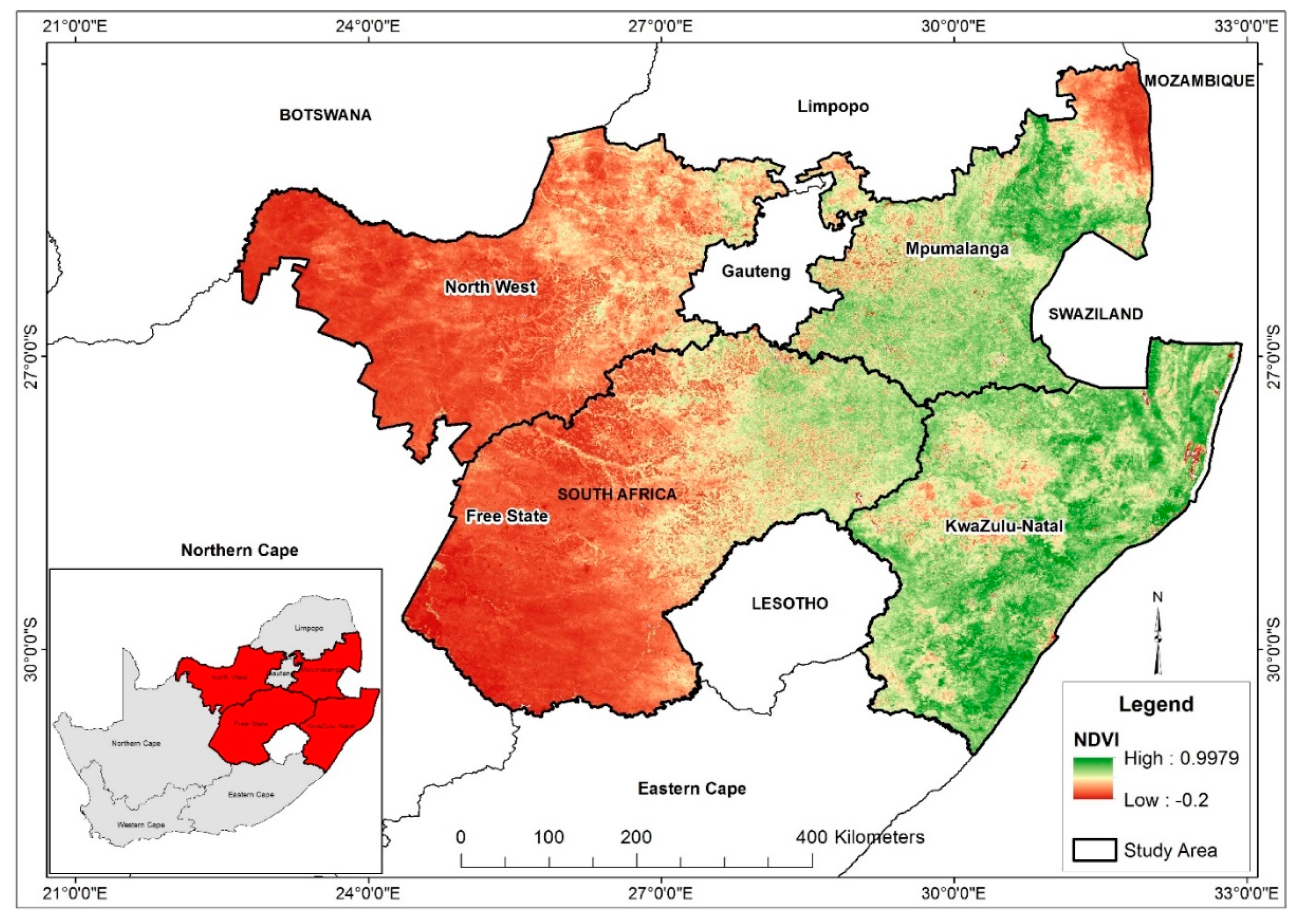
Maize is considered to be the most important grain crop, a staple food for a large proportion of the population and a major input to animal feed in South Africa. In South Africa, maize is produced by both commercial and subsistence farmers and accounts for about 45% of the gross domestic product of the agricultural sector. About 8 million tons of maize grain is produced annually in the country under varying soil, terrain, and climatic conditions. Free State (FS), North West (NW), Mpumalanga (MP) and KwaZulu-Natal (KZN) are the major maize producing provinces in South Africa accounting for about 83% of the total national production. FS and NW provinces both contribute over 60%, followed by MP (~24%) and KZN (less than 5%) [19].

Furthermore, the Food and Agriculture Organization of the United Nations (FAO) has recently reported maize as the largest grain crop (in metric tons) produced in the world [20]. Therefore, in order to ensure food security for a rapidly growing population, in the face of climate variability, several studies have been conducted on maize ranging from climate influence on maize to yield predictions. To this end, numerous researchers across the globe have used ANNs to predict maize yield and have proven this method to be reliable. For instance, Maryland’s corn and soybean were predicted by developing a feed-forward back-propagation ANN model using the rainfall and soil properties [21]. Similarly, [14] predicted maize yield at three scales in east-central Indiana, USA, with local crop-stage weather and yield data spanning from 1901 to 1996 using a fully connected back-propagation ANN together with regression models. In addition, [22] developed a feed-forward neural network to estimate the nonlinear relationship between soil parameters and crop yield. The results indicated a relatively high degree of accuracy for crop yield prediction. Furthermore, a study by [23] in eastern Ontario, Canada, evaluated the predicting power of ANN for corn and soybean yield using remotely sensed variables. The model was found to report an error level below 20% indicating the reliability of the model in predicting corn and soybean yield. Using climate data and fertilizer as predictors, [24] predicted maize yield in Jilin, China. The authors reported a close similarity between the predicted yield and the observed yield. Despite proven reliability of the application of ANNs to maize yield production, only a few studies have used these models for predicting maize yield in South Africa. Many of the existing studies have relied on the use of crop-based models which are in most cases expensive and data intensive. The aim of this study is to develop an artificial neural network for predicting maize yield in the major maize producing areas of South Africa (FS, NW, MP, and KZN).

2. Materials and Methods

2.1. Study Area

The study area includes the north-eastern part of South Africa between longitude 22° E to 33° E and latitude −32° S to −24° S. It covers KZN, FS, MP, and NW provinces, see Figure 1. Agriculture dominates the FS landscape. This is attributed to the fact that the province is agro-ecologically located on a flat plain with approximately 5% slopes. It is about 1300 m above sea level, characterized by summer rainfall (500–600 mm annually), temperature ranging between 1 °C to mild 17 °C in winter and 15 °C to 32 °C in summer. As the FS has more than 30,000 farmers producing over 70% of the country’s grain, hence the province is referred to as the “Heart and Bread-Basket of the Country”.

The NW province is considered to be an important contributor to the South Africa food basket with an estimated 43.9% of the province categorized as “arable” land. There are three distinct climatic regions which allow a wide variety of agricultural activity. The drier western region (hunting, cattle, and game farming), the central and southern parts (maize, wheat and cash crops) and the eastern and north-eastern region (variety of crops). The province is characterized by almost all year-round sunshine, rainfall ranges between 300 and 700 mm per annum, summer temperature ranging from 22 °C to 34 °C and winter temperature ranging from 2 °C to 34 °C. The MP province is rated as one of South Africa’s most important and productive agricultural regions. The province is characterized by rainfall of about 500 reaching up to 800 mm per annum with an average temperature of about 19 °C. In KZN the land area devoted to grain and seed production varies yearly according to the price of crops, demand and supply, and annual rainfall received. The province is characterized by long, hot summer with temperature ranging from 23 °C to 33 °C, winter temperature ranging from 16 °C to 25 °C, and an average annual rainfall of 500 to 800 mm [25].

2.2. Datasets

The datasets used in this study are: the Normalized Difference Vegetation Index (NDVI), potential evapotranspiration (PET), precipitation (PRE), minimum temperature (TMN), maximum temperature (TMX), soil moisture (SM), size of land cultivated for maize production (Land) and maize production per province (P) as the dependent variable. The PET, PRE, TMN, and TMX datasets were acquired from the Climate Research Unit Time-Series 3.24.01 (CRU TS 3.24.01). These data were derived from monthly observations from over 4000 meteorological stations distributed across the world’s land areas. The gridded CRU TS 3.24.01 product is freely available for the science community on http://badc.nerc.ac.uk/data/cru or http://www.cru.uea.ac.uk. The reader is referred to [26] for more details on the construction of the CRU TS 3.24.01 product. The SM data was acquired from the European Space Agency (ESA), as part of their Climate Change Initiative (CCI) program. This product is a combination of both active and passive microwave sensors. It has a spatial resolution of 0.25 degrees, given in volumetric units (m³ m⁻³) and is provided in NetCDF-4 format. Maize production data sets per province in tons (tons), as well as the land area cultivated in hectares (ha) for maize production for the major maize-producing provinces were obtained from the abstract of agricultural statistics compiled by the Department of Agriculture, Forestry and Fisheries of South Africa (DAFF). This abstract document contains important information on inter alia, field crops, horticulture, livestock, vital indicators, total land area in hectares (ha) cultivated for maize production, and the contribution of primary agriculture to the South African economy. The data are available on the department’s website (www.daff.gov.za). All datasets are extracted monthly and are averaged from October to April (average maize growing period in South Africa). This was done to ensure the same data scale as the maize data which was collected yearly. All datasets span from 1990–2017. Summary of the input data is given in

Table 1. Summary of input data used for this study.

Data Names	Abbreviation	Sources
Normalized Difference Vegetation Index	NDVI	MODIS (MOD13Q1)
Potential Evapotranspiration	PET	Climate Research Unit
Precipitation	PRE	Climate Research Unit
Minimum Temperature	TMN	Climate Research Unit
Maximum Temperature	TMX	Climate Research Unit
Soil Moisture	SM	European Space Agency
Size of land cultivated for maize production	Land	Department of Agriculture, Forestry and Fisheries

.

2.3. Data Analysis

Artificial Neural Network

In this study, the input variables include the PET, PRE, TMN, TMX, SM, and land cultivated for maize production. The mathematical model is presented in Equation (1), where; y is the output, x₁, x₂ ……. x_n represents the input variables, w₁, w₂ ……. w_n represents the weights of the combination which generates the output, $\theta$(.) is the unit step function, $w_i$ are the weights related with the ith input and $\mu$ is the mean.

$$y=\theta {\displaystyle \sum }_{j=1}^n{w}_i{x}_i-\mu$$

(1)

The generalized weight $w_i$ is defined as the contribution of the $i$th covariate to the log-odds, and was introduced by [27]. The equation below represents the generalized weight:

$$w_i=\frac{\partial \log \left(\frac{o\left(x\right)}{1-o\left(x\right)}\right)}{\partial x_i}$$

(2)

where the generalized weight shows the effect of the individual covariate $x_i$ and consequently has an analogous interpretation as the $i\mathrm{th}$ regression parameter in regression models, $o\left(x\right)$ is the predicted outcome probability by covariate vector and log-odds is the link function for the logistic regression model. Note that, the generalized weight depends on all other covariates.

The analysis was performed using the neuralnet package in R software. The neuralnet uses the supervised learning algorithms which comprise a flexible function that trains multilayer perceptron to a particular data set [28]. A two layer back propagation network with sufficient hidden nodes that has been proven to be a universal approximator was adopted [22,27]. The data were scaled in order to nullify the ambiguous effect that a variable might have on the prediction variable due to its scale. Hence, the min-max normalization was used to transform the data into a common range, thereby removing the scaling effect from all the variables. Both the dependent variable (maize) and independent variables were partitioned into training and test datasets. The training data consist of the 80% of the data (1990 to 2011) while the test data is 20% of the data (2012 to 2017). The training data is the set of data from which the system learns from and testing data is used to validate the model’s performance by comparing the predicted maize yield with the actual maize yield. In order to improve the performance of the neural network different combinations of the input variables (PET, PRE, TMN, TMX, SM, and Land) with a vector (hidden neuron); (indicating the number of hidden layers and hidden neurons in each layer) were used with an automated loop to change the vector (architecture) for each province. Hence, the best combination of variables and architecture for each province was selected using the percentage of accuracy. The best combination for each province was then used to predict maize production and was compared with the testing data (20%) left out from the machine learning process. The projection was made using the avNNet function in Caret package in R. The performance measures of the prediction were accessed using the adjusted R². The projection for maize production for the years 2018 and 2019 was then performed.

3. Results

3.1. Optimizing Combinations of Variable Selection

Owing to the fact that there is no standard method for the selection of variables in the neuron network, it is usually done by testing various variable combinations so as to arrive at the best combination for the model. In this case, as reported by [29], the major agro-climatic variable that influences maize yield varies across the maize producing areas of South Africa. According to the current study, the TMX is the major determinant in the FS and MP provinces, while the TMN is largely responsible for changes in maize yield in the NW province. Both the PET and TMN are found to be the major drivers of maize yield in KZN. These variables were selected as a baseline for the variable combination check, by holding them constant in all the combinations. Since six variables (i.e., PET, PRE, TMN, TMX, Land and SM) were used in the model, 12 combinations were created for each province except for KZN province, which had just 10 because two climatic variables largely determine its maize yield.

Table 2. Top five architecture of hidden configurations from different variable combinations; with scores, rank and the root mean squared error (RMSE) (Scores refers to the accuracy level (%) of the combination with the hidden neuron and ranked 1 to 5 accordingly).

Province	Combination of Variables	Hidden Neuron	Scores	Rank	RMSE
FS	TMX, Land, SM	8,9	76.64%	1	0.0383
		5,9	76.55%	2	0.0397
		5,7	76.28%	3	0.0381
		3,6	76.18%	4	0.0382
		7,8	76.13%	5	0.0393
	PET, PRE, TMN, TMX, Land, SM	5,8	82.42%	1	0.0374
		6,7	82.41%	2	0.0472
		4,9	82.02%	3	0.0445
		6,8	82.01%	4	0.041
		3,8	81.43%	5	0.0399
	PRE, TMN, TMX, Land, SM	2,6	82.46%	1	0.0347
		4,9	81.94%	2	0.0456
		4,5	80.80%	3	0.0457
		6,7	80.79%	4	0.0429
		8,9	79.19%	5	0.0483
NW	PRE, SM, TMN	5,6	71.51%	1	0.014
		3,5	71.26%	2	0.0166
		5,6	70.16%	3	0.0202
		6,9	69.99%	4	0.0152
		7,9	69.10%	5	0.0158
	TMN, Land, SM	3,4	73.74%	1	0.015
		2,5	72.33%	2	0.0179
		7,9	67.82%	3	0.0178
		3,6	67.77%	4	0.0172
		1,9	67.59%	5	0.0176
	TMN, SM	2,8	69.22%	1	0.0142
		4,9	69.06%	2	0.0147
		8,9	67.52%	3	0.0152
		3,8	67.08%	4	0.0170
		3,5	67.99%	5	0.0161
MP	TMN, TMX, Land, SM	3,4	93.79%	1	0.024
		3,5	91.02%	2	0.0267
		2,7	90.77%	3	0.0267
		6,9	90.73%	4	0.0271
		3,8	90.61%	5	0.0275
	PET, PRE, TMN, TMX, Land	7,9	92.02%	1	0.0243
		2,6	91.08%	2	0.0267
		4,9	90.64%	3	0.0273
		1,8	90.35%	4	0.0283
		1,4	89.99%	5	0.0262
	PET, TMX	4,7	88.39%	1	0.0246
		2,7	88.16%	2	0.0247
		8,9	87.77%	3	0.0248
		1,8	87.53%	4	0.0250
		3,8	87.51%	5	0.0245
KZN	PET, PRE, TMN, TMX	3,5	89.90%	1	0.0055
		4,6	89.66%	2	0.0055
		3,6	89.05%	3	0.0055
		3,9	88.95%	4	0.0055
		3,4	88.93%	5	0.0057
	PET, TMN, TMX, Land, SM	1,8	61.23%	1	0.0036
		1,9	61.20%	2	0.0036
		1,3	60.94%	3	0.0036
		3,5	47.19%	4	0.0036
		4,7	45.59%	5	0.0036
	PET, PRE, TMN, TMX, Land, SM	7,8	93.90%	1	0.0033
		4,7	92.15%	2	0.0037
		5,8	91.47%	3	0.0052
		4,5	90.64%	4	0.0055
		2,9	90.18%	5	0.0060

illustrate the combination of variables, the hidden neuron, overall error, and accuracy of the best three ranked combinations that best predict maize yield in each of the provinces.

According to Table 2, in the FS province, the combination of TMX, Land and SM variables at different automated two hidden neurons with vector (8,9) ranked first within this group with 76.64% accuracy and has a root mean squared error (RMSE) of 0.038. The combination of the PET, PRE, TMN, TMX, Land and SM using vector (5,8) resulted in an accuracy of 82.42% and RMSE of 0.037 and ranked first. On the other hand, an accuracy of 82.46% and RMSE of 0.035 was achieved when PRE, TMN, TMX, Land and SM were combined using vector (2,6). Hence, the combination of variables PRE, TMN, TMX, Land and SM with vector (2,6) was chosen to model maize production for the FS province. For the NW province, the combination of only two variables TMN and SM using vector (2,8) gave an accuracy of 69.22% and had RMSE of 0.014. When PRE was added to TMN and SM but with vector (5,6) the accuracy improved to 71.51% with RMSE of 0.014. However, a higher accuracy of 73.74% with RMSE of 0.015 was attained with the variable combination of TMN, Land, and SM with vector (3,4). Considering the combination with the highest accuracy, a variable combination of TMN, Land and SM with vector (3,4) was selected for the model for the NW province.

Furthermore, for MP province, the combination of variables PET and TMX using vector (4,7) gave an accuracy of 88.39% and RMSE of 0.025. The accuracy for a variable combination that better combined to predict maize yield improved to 92.02% when PET, PRE, TMN, TMX and Land were combined. The accuracy further improved to 93.79% with RMSE of 0.024 when variables TMN, TMX, Land and SM were combined using vector (3,4). Consequently, the combination of TMN, TMX, Land and SM with vector (3,4) were selected as the model for MP province. In the case of KZN, the combination of PET, TMN, TMX, Land, and SM with vector (1,8) produced an accuracy of 61.23% and RMSE of 0.0036. When the PET, PRE, TMN and TMX were combined with vector (3,5) an accuracy of 89.39% was achieved. However, the combination of PET, PRE, TMN, TMX, Land, and SM using vector (7,8) gave 93.90% accuracy and RMSE of 0.003 in predicting maize yield in KZN. Therefore, the combination of the PET, PRE, TMN, TMX, Land and SM variables with two hidden neurons of (7,8) was selected for the model for KZN province.

3.2. Generalized Weight of the Variables $(w_i)$

Table 3. Generalized weight for the independent variable in Free State.

Year	PRE	TMX	TMN	Land	SM
1990	0.09	1.18	0.03	1.02	−0.99
1991	0.09	0.88	−0.10	0.97	−0.88
1992	0.04	0.35	−0.07	0.45	−0.40
1993	0.01	0.28	0.04	0.19	−0.20
1994	0.42	7.88	1.05	5.24	−5.56
1995	0.05	0.52	−0.05	0.56	−0.52
1996	0.02	1.87	0.61	0.58	−0.86
1997	0.06	2.44	0.65	1.04	−1.32
1998	0.05	0.75	0.03	0.62	−0.61
1999	0.02	0.24	0.01	0.20	−0.20
2000	0.12	1.53	0.01	1.37	−1.32
2001	0.05	0.73	0.06	0.55	−0.56
2002	0.07	1.37	0.18	0.91	−0.96
2003	0.13	1.16	−0.14	1.32	−1.20
2004	0.13	1.10	−0.20	1.37	−1.22
2005	0.22	1.62	−0.39	2.18	−1.90
2006	0.17	2.16	0.03	1.91	−1.86
2007	0.04	0.59	0.04	0.47	−0.47
2008	0.08	1.27	0.10	0.96	−0.98
2009	0.04	0.37	−0.05	0.42	−0.38
2010	0.13	1.20	−0.14	1.35	−1.23
2011	0.07	0.76	−0.02	0.72	−0.69

,

Table 4. Generalized weight for the independent variable in North West.

Year	TMN	Land	SM
1990	1.12	0.37	−0.95
1991	1.41	0.38	−1.29
1992	1.52	0.39	−1.51
1993	1.70	0.43	−1.52
1994	1.43	0.39	−1.34
1995	1.62	0.48	−1.55
1996	1.66	0.42	−1.41
1997	1.58	0.42	−1.38
1998	1.59	0.43	−1.47
1999	1.66	0.49	−1.35
2000	1.59	0.49	−1.42
2001	1.53	0.54	−1.43
2002	1.36	0.36	−1.33
2003	1.39	0.36	−1.36
2004	1.41	0.37	−1.38
2005	1.44	0.40	−1.34
2006	1.47	0.41	−1.38
2007	1.44	0.39	−1.38
2008	1.26	0.39	−1.12
2009	1.47	0.40	−1.42
2010	1.41	0.40	−1.29
2011	1.50	0.42	−1.40

,

Table 5. Generalized weight for the independent variable in Mpumalanga.

Year	TMX	TMN	Land	SM
1990	1.62	−0.44	−0.08	−0.45
1991	1.67	−0.45	−0.08	−0.47
1992	1.19	−0.25	−0.03	−0.40
1993	1.73	−0.61	−0.11	−0.47
1994	2.01	−0.76	−0.14	−0.51
1995	1.71	−0.51	−0.09	−0.47
1996	2.23	−0.92	−0.18	−0.54
1997	1.98	−0.73	−0.14	−0.51
1998	1.81	−0.56	−0.10	−0.50
1999	2.11	−0.78	−0.15	−0.53
2000	2.14	−1.03	−0.20	−0.50
2001	1.70	−0.79	−0.15	−0.41
2002	1.76	−0.59	−0.11	−0.47
2003	1.29	−0.16	−0.01	−0.43
2004	1.75	−0.52	−0.09	−0.49
2005	1.55	−0.41	−0.07	−0.46
2006	1.97	−0.69	−0.12	−0.51
2007	1.32	−0.26	−0.03	−0.43
2008	1.51	−0.49	−0.09	−0.41
2009	1.66	−0.44	−0.08	−0.48
2010	1.58	−0.38	−0.06	−0.46
2011	1.34	−0.50	−0.08	−0.38

and

Table 6. Generalized weight for the independent variable in KwaZulu-Natal.

Year	PET	PRE	TMX	TMN	Land	SM
1990	−1.69	0.63	2.93	−1.66	1.00	−2.97
1991	−5.33	0.92	8.76	−0.56	2.95	−5.37
1992	−1.78	0.59	3.00	0.31	1.31	−2.05
1993	−1.17	0.55	2.08	0.18	0.95	−1.66
1994	−5.02	1.06	8.00	0.91	2.92	−4.88
1995	−2.69	0.64	4.57	−0.83	1.57	−3.26
1996	−1.74	0.69	3.28	−0.29	1.35	−2.40
1997	−2.28	0.71	4.01	0.26	1.58	−2.60
1998	−2.03	0.69	3.60	0.37	1.49	−2.33
1999	−3.18	0.76	5.06	0.54	1.99	−3.24
2000	−6.22	0.59	8.49	1.81	2.41	−5.09
2001	−3.80	0.68	5.82	1.00	1.90	−3.53
2002	−1.33	0.50	2.28	−0.02	0.93	−1.81
2003	−1.43	0.54	2.42	−0.09	0.99	−1.97
2004	−1.25	0.55	2.13	−0.93	0.79	−2.26
2005	−1.54	0.64	2.78	−0.07	1.22	−2.12
2006	−1.63	0.59	2.90	0.28	1.22	−1.96
2007	−1.33	0.42	2.01	0.26	0.76	−1.67
2008	−1.47	0.55	2.48	−0.98	0.89	−2.43
2009	−1.04	0.59	1.95	−0.32	0.87	−1.87
2010	−1.21	0.62	2.33	0.13	1.14	−1.72
2011	−1.35	0.51	2.43	0.20	1.13	−1.61

show the generalized weight expressing the effect of each independent variable on the dependent variable in the combination. As shown in Table 3, PRE, TMX and Land have a positive linear effect on maize production for all the trained years in the FS province. This indicates a favorable relationship between PRE, TMX, Land and maize production in the area with variance ranging from 0.01 to 0.42, 0.24 to 7.88 and 0.19 to 5.24 for PRE, TMX and Land, respectively. A negative effect is noticed between SM and maize production with variance ranging from −5.56 to −0.20, suggesting an unfavorable relationship between the two variables. Similarly, there exist both negative (40.91%) and positive (59.09%) effects between TMN and maize production for the trained year. The relationship was negative for years 1991, 1992, 1995, 2003, 2004, 2005, 2009, 2010, and 2011 with its variance ranging from −5.56 to −0.20, suggesting an unfavorable relationship between the two variables in those corresponding years.

The generalized weight for the independent variables for the NW province is shown in Table 4. Both TMN and Land depict a positive linear effect on maize production in the province with variance ranging from 1.12 to 1.70 and 0.36 to 0.54, respectively. This suggests a favorable relationship between the two independent variables and maize production in the province. On the other hand, SM has a negative linear effect on maize production in the province with the variance ranging from −1.55 to −0.95. This implies an unfavorable relationship between the two variables.

Table 5 depicts the generalized weight for the independent variables in MP province. The TMX depicts a positive linear effect on maize production in the province with its variance ranging from 1.19 to 2.23. This implies that TMX has a favorable relationship with maize production. However, TMN, Land and SM display a negative linear effect on maize production with their variance ranging from −1.03 to −0.25, −0.20 to −0.01 and −54 to −0.38, respectively. Thus, these variables have an unfavorable relationship with maize production in the province.

As depicted in Table 6, the PET and SM have a negative linear effect on maize production in KZN province with their variance ranging from −6.22 to −1.04 and −5.37 to −1.61, respectively. Therefore, these variables have an unfavorable relationship with maize production in the area. The following variables PRE, TMX, and Land display a positive linear effect on maize production in the province and their variances range from 0.42 to 1.06, 1.95 to 8.76 and 0.76 to 2.95, respectively. The case is different for TMN where 45.45% of this variable has a negative linear effect on maize production in the area as its variance ranges from −1.66 to −0.02. The remaining 54.55% has a positive linear effect on maize production in the province and its variance ranges from 0.13 to approximately 1.81.

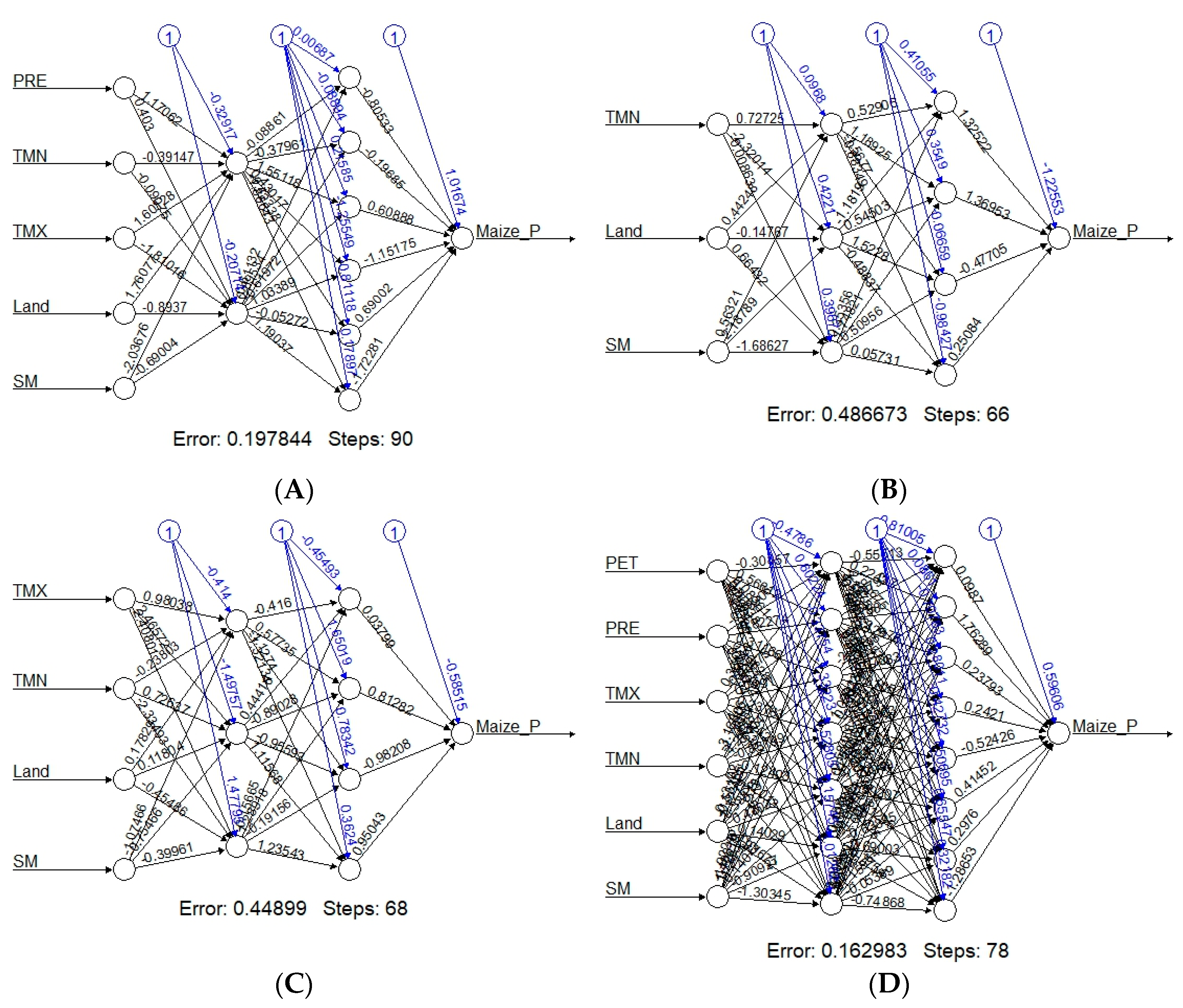
3.3. Network Topology

The training process results are illustrated in Figure 2A–D. The figure reflects the structure of the trained neural network for each province. The network topology conveys basic information such as the trained synaptic weights, the number of steps needed for converge and the overall errors. For the purpose of this study, the threshold for the partial derivatives of the error function was set at 0.01. Each province has its own unique variable combinations as well as hidden neurons (see Table 2; i.e., the FS province has PRE, TMN, TMX Land and SM with hidden neuron c(2,6); NW province TMN, Land and SM with hidden neuron c(3,4); MP province TMN, TMX, Land, and SM with hidden neuron c(3,4); and KZN province PET, PRE, TMN, TMX, Land and SM with hidden neuron c(7,8).

Figure 2A shows that in the FS province, the training process needed 90 steps to achieve less error function (i.e., < threshold of 0.01). The process has an overall error of about 0.20. In the NW province, according to Figure 2B, the training process needed 66 steps until all absolute partial derivative of the error function were smaller than 0.01 with the process having an overall error of about 0.49. On the other hand, in MP province (Figure 2C), the training process needed 68 steps until all absolute partial derivatives of the error function were smaller than the default threshold of 0.01 with the process having an overall error of about 0.45. In KZN (see Figure 2D) the training process needed 78 steps until all absolute partial derivatives of the error function were smaller than 0.01, and the overall error was 0.16.

3.4. Maize Prediction and Validation

Having trained the neural network with 80% of both the independent and dependent variables, and the best combinations with the hidden neuron selected, the prediction for maize production per province was made for the same time frame (2012–2017) of the testing data (20%). The predicted output was then compared with the reserved 20% that was not used for machine learning. The results are displayed in

Table 7. Comparison between predicted and actual maize production for Free State (“000” tons).

Year	Actual Maize Production	Predicted Maize Production	Difference (Predicted-Actual)	Deviation
2012	4884.8	4254.24	−630.56	−0.13
2013	6247.25	4146.92	−2100.33	−0.34
2014	3945	3939.01	−5.99	−0.002
2015	2213.5	2789.29	575.79	0.26
2016	7330.5	3961.63	−3368.87	−0.46
2017	5515.9	3844.02	−1671.88	−0.30

,

Table 8. Comparison between predicted and actual maize production for North West (“000” tons).

Year	Actual Maize Production	Predicted Maize Production	Difference (Predicted-Actual)	Deviation
2012	1613	1671.57	58.57	0.04
2013	2898	1956.05	−941.95	−0.33
2014	1490	1830.38	340.38	0.23
2015	1141	1416.96	275.96	0.24
2016	3135	1934.21	−1200.79	−0.38
2017	2123.5	1841.02	−282.48	−0.13

,

Table 9. Comparison between predicted and actual maize production for Mpumalanga (“000” tons).

Year	Actual Maize Production	Predicted Maize Production	Difference (Predicted-Actual)	Deviation
2012	3005	2721.47	−283.53	−0.09
2013	2782.2	2552.24	−229.96	−0.08
2014	2429.3	2192.19	−237.11	−0.10
2015	2319	2308.74	−10.26	−0.004
2016	3431	2761.67	−669.33	−0.20
2017	2880	2670.98	−209.02	−0.07

and

Table 10. Comparison between predicted and actual maize production for KwaZulu-Natal (“000” tons).

Year	Actual Maize Production	Predicted Maize Production	Difference (Predicted-Actual)	Deviation
2012	599	520.82	−78.18	−0.13
2013	559.1	541.99	−17.11	−0.03
2014	507.5	476.63	−30.87	−0.06
2015	522	468.26	−53.74	−0.10
2016	735	572.21	−162.79	−0.22
2017	682.5	615.61	−66.89	−0.10

. The accuracy level of the prediction varies for each province. For instance, the model for the FS province has an adjusted R² of 0.75, and NW, MP and KZN provinces have an R² of 0.67, 0.86 and 0.82, respectively.

As depicted in Table 7, the predicted maize production in the FS province deviated from the actual maize production by −0.13 (13%), −0.34 (34%), −0.002 (0.2%), −0.46 (46%) and −0.30 (30%) for years 2012, 2013, 2014, 2016, and 2017, respectively. The results suggest an under-prediction of maize production in the province. On the other hand, 2015 resulted in over-prediction (i.e., 0.26 which is equivalent to 26%) of maize production.

As shown in Table 8, the predicted maize production for the NW province deviated from the actual maize production by −0.33 (33%), −0.38 (38%), and −0.13 (13%) for 2013, 2016 and 2017 respectively, thus there was under-prediction of maize production. Contrasting this, maize production was over-predicted by 0.04 (4%), 0.23 (23%) and 0.24 (24%) in 2012, 2014 and 2015, respectively.

From Table 9, maize production is under-predicted for the MP province across the entire testing period by −0.09 (9%), −0.08 (12%), −0.10 (10%), −0.004 (0.4%), −0.20 (20%) and −0.07 (7%) for the years 2012, 2013, 2014, 2015, 2016, and 2017, respectively.

In KZN province according to the results presented in Table 10, maize production was under-predicted by −0.13 (13%), −0.03 (3%), −0.06 (6%), −0.10 (10%), −0.22 (22%) and −0.10 (10%) in 2012, 2013, 2014, 2015, 2016 and 2017, respectively.

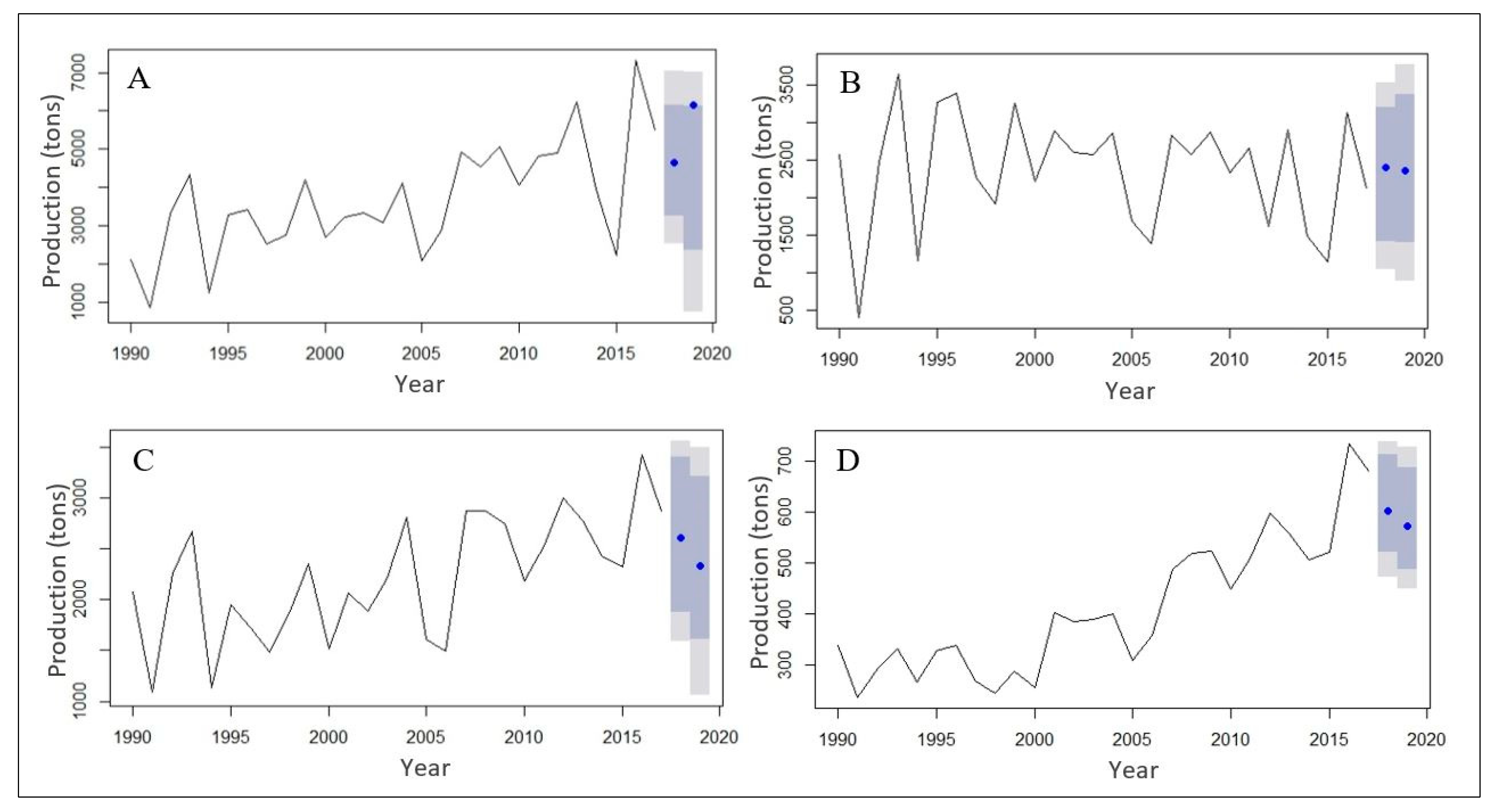
3.5. Maize Production Projection

The results of the projected maize production performed with AvNNet() in Caret package across each province for the year 2018 and 2019 is shown in Figure 3A–D and

Table 11. Projected maize production for FS: Free State, NW: North West, MP: Mpumalanga and KZN: KwaZulu-Natal for 2018 and 2019 using the best variable combinations for each province (“000” tons).

Year	FS	NW	MP	KZN
2018	4651.03	2403.94	2604.34	602.73
2019	6146.33	2361.61	2335.61	572.74
Difference	1495.3	−42.33	−268.73	−29.99
Deviation	0.32	−0.02	−0.10	−0.05

. The results indicate that maize production will decrease across all the provinces (except FS) from the current year 2017 to 2018 and 2019. The FS depicts a 32% increase in maize production, i.e., from 2018 (4651.03 tons) to 2019 (6146.33 tons). In Figure 3A–D, the dark gray shaded and light gray shaded area is the 80% and 95% prediction confidence interval, respectively.

4. Discussion

In this study, maize production in the FS, NW, MP and KZN provinces of South Africa was modeled based on the ANN approach. The analysis considered various variable combinations and ranked the accuracy of these combinations across the study area. The results indicated spatial dependence of different combinations in different provinces. For instance, the PRE, TMN, TMX, Land and SM with hidden neuron c(2,6) combination were ranked first in the FS province; TMN, Land and SM with hidden neuron c(3,4) in the NW province; TMN, TMX, Land, and SM with hidden neuron c(3,4) in MP and lastly, PET, PRE, TMN, TMX, Land and SM with hidden neuron c(7,8) ranked first in KZN. The three variables, i.e., TMN, Land and SM, seem to dominate in all first ranked levels across all the four provinces.

Maize production in the four selected provinces is highly affected by different agro-climatic parameters, as reported in [29]. In this study, we found that TMX is the main driver of change in maize yield in the FS and MP, whereas TMN has a dominant impact in the NW. The PET and TMN climate variables dominate in KZN, hence significantly affecting the maize yield in the province. The results indicate that the variables have a linear effect on maize production since their variance was very small. In addition, the influence of TMN on maize production varied in the NW, FS and KZN, having a positive linear effect. However, the TMN in MP exhibited a negative linear effect on maize production. The land has a positive linear effect on maize production across all the provinces except for MP where it has a negative linear effect. Similarly, SM exhibited a negative linear effect on maize production across all the provinces. The TMX displayed a positive linear effect on maize production in the FS, MP and KZN. PRE appeared in the variable combination of just two provinces (FS and KZN) and it has a positive linear effect on maize production in both of these provinces.

The accuracy of the combined variables to predict maize production varied across the provinces. The accuracy was recorded in MP (93.79%) and KZN (93.90%). This accuracy suggests that the TMN, TMX, Land and SM are sufficient for modelling maize production in MP province while PET, PRE, TMN, TMX, Land and SM are ideal for the effective modelling of maize production in KZN. Nevertheless, these results do not extensively mean that other farm management practices such as fertilizer application, irrigation and choice of cultivar are not significant in achieving best output for maize production. They are thought to account for the deviations in the comparison between the actual and predicted maize production. On the other hand, despite the high accuracy of about 82.46% of the combined variables of PRE, TMN, TMX, Land and SM to predict maize production in the FS, a high deviation is noticed between the actual maize production and predicted production particularly in the year 2016 where maize is up by 46%. These results are in contrast with the deviation between actual and predicted maize production in the NW where the selected combination of TMN, Land and SM gave an accuracy of 73.74% but gave a smaller deviation between actual and predicted maize production. This could suggest that the FS province is more prone to the influence of other farm management practices.

The projected maize production indicates that maize production is on the decline across all the provinces. This can be attributed to the future trend of changes in climatic variables as well as a projected increase in drought occurrences [29,30].

5. Conclusions

This study demonstrates the value of the artificial neural network in predicting maize yield across the four major maize producing provinces of South Africa. These results agree with the previous research findings [27]. The results indicate that different climatic variables and/or their combinations serve(s) as major drivers for maize production across the different provinces. The accuracy level of the prediction obtained between the actual and predicted maize production for each province as given by the adjusted R² value, with 0.75 in the FS, 0.67 in the NW, 0.86 in MP and 0.82 in KZN. In this study, the adjusted R² is used as a measure of future prediction of maize production.

Although the predicted maize production is under-predicted, we conclude that it is better to under-predict than over-predict. This is because an under-prediction will enhance the decision making process of the farmers and/or the policymakers to put in place measures to ensure that loss of production is prevented or minimized, rather than be blinded by expectation of high production. In addition, all the predictions (under-predictions), particularly in MP and KZN, are within 10% of the actual maize production except for the year 2016, in which the production was approximately 20%.

The decline in projected maize production can be attributed to the effects of climate change and variability; hence adequate adaptation and coping measures are needed for both commercial and small-scale farmers to prevent loss of production and aggravated famine.

This research study is essential in South Africa, as food security is threatened by drought due to climate change and variability. The availability of historical and current agro-climatic data combined in a model could serve as a vital decision support system to cope and mitigate climate change. The model is developed to incorporate different farming scenarios such as the combination of agro-climatic parameters with different farming practices to predict maize yield. Hence, this tool can help farmers to make informed choices, which include mitigation and adaptation measures in order to maximize profit on crop production. Furthermore, the model will be operationalized and made available to relevant stakeholders and decision makers such as commercial and small-scale farmers and the Department of Agriculture.

This study can be improved to ensure its operability by incorporating other farm management practices such as fertilizer application that was not available/accessible during the period of undertaking this research. However, the current status of this model can be validated by comparing the projected production of maize with the actual production at the end of the 2018 and 2019 season.

References

1. World Wildlife Fund. Meeting Report and Recommendations. From the Sustainable Food for the 21st Century Advisory Panel; World Wildlife Fund: Washington, DC, USA, 2018. [Google Scholar]
2. Lobell, D.B.; Field, C.B. Global scale climate crop yield relationships and the impacts of recent warming. Environ. Res. Lett. 2007, 2, 014002. [Google Scholar] [CrossRef]
3. Fortin, J.G.; Anctil, F.; Parent, L.E.; Bolinder, M.A. Site-specific early season potato yield forecast by neural network in Eastern Canada. Precis. Agric. 2011, 12, 905–923. [Google Scholar] [CrossRef]
4. Alvarez, R. Predicting average regional yield and production of wheat in the Argentine Pampas by an artificial neural network approach. Eur. J. Agron. 2009, 30, 70–77. [Google Scholar] [CrossRef]
5. Yang, C.; Peterson, C.L.; Shropshire, G.J.; Otawa, T. Spatial variability of field topography and wheat yield in the Paleous region of the Pacific Northwest. Trans. ASAE 1998, 41, 17–27. [Google Scholar] [CrossRef]
6. Ghodsi, R.; Yani, R.M.; Jalali, R.; Ruzbahman, M. Predicting wheat production in Iran using an artificial neural networks approach. Int. J. Acad. Res. Bus. Soc. Sci. 2012, 2, 34–47. [Google Scholar]
7. Paswan, R.P.; Begum, S.A. Regression and neural networks models for prediction of crop production. IJSER 2013, 4, 2229–5518. [Google Scholar]
8. Dalgliesh, N.; Saifuzzaman, M.; Khan, I.; Hossain, A.B.S.; Rawson, H. Expanding the Area for Rabi-Season Cropping in Southern Bangladesh; Final Report LWR/2005/146; Australian Centre for International Agricultural Research (ACIAR): Canberra, Australia, 2012.
9. Gonzalez-Sanchez, A.; Frausto-Solis, J.; Ojeda-Bustamante, W. Attribute selection impact on linear and nonlinear regression models for crop yield prediction. Sci. World J. 2014, 2014, 509249. [Google Scholar] [CrossRef] [PubMed]
10. Abdipour, M.; Younessi-Hmazekhanlu, M.; Ramazani, S.H.R.; Omidi, A.H. Artificial neural networks and multiple linear regression as potential methods for modeling seed yield of safflower (Carthamus tinctorius L.). Ind. Crops Prod. 2019, 127, 185–194. [Google Scholar] [CrossRef]
11. Klemme, R.M. An Econometric Yield Response and Forecasting Model for Corn in Indiana. Master’s Thesis, Purdue University, West Lafayette, IN, USA, August 1978. [Google Scholar]
12. Molazem, D.; Valizadeh, M.; Zaefizadeh, M. North West of genetic diversity of wheat. J. Agric. Sci. 2002, 20, 353–365. [Google Scholar]
13. Zaefizadeh, M.; Khayatnezhad, M.; Gholamin, R. Comparison of multiple linear regressions and artificial neural network in predicting the yield using its components in the Hassle Barley. Am.-Eurasian J. Agric. Environ. Sci. 2011, 10, 60–64. [Google Scholar]
14. O’Neal, M.R.; Engel, B.A.; Ess, D.R.; Frankenberger, J.R. Neural network prediction of maize yield using alternative data coding algorithms. Biosyst. Eng. 2002, 83, 31–46. [Google Scholar]
15. Caselli, M.; Trizio, L.; de Gennaro, G.; Ielpo, P. A simple feedforward neural network for the PM10 forecasting: comparison with a radial basis function network and a multivariate linear regression model. Water Air Soil Pollut. 2009, 201, 365–377. [Google Scholar] [CrossRef]
16. Liu, J.; Goering, C.E. Neural network for setting target corn yields. Presented at the ASAE Annual International Meeting, St. Joseph, MI, USA, 18–21 July 1999. [Google Scholar]
17. Liu, J.; Goering, C.E.; Tian, L. A neural network for setting target corn yields. Trans. ASAE. 2001, 44, 705–713. [Google Scholar]
18. Hsieh, W.W. Machine Learning Methods in the Environmental Sciences: Neural Networks and Kernels; Cambridge University Press: New York, NY, USA, 2009; p. 349. [Google Scholar]
19. DAFF (Department of Agriculture, Forestry and Fishery). Trends in the Agricultural Sector. Available online: https://www.daff.gov.za/Daffweb3/Portals/0/Statistics%20and%20Economic%20Analysis/Statistical%20Information/Trends%20in%20the%20Agricultural%20Sector%202017.pdf (accessed on 11 July 2018).
20. Food and Agriculture Organization of the United Nations (FAO). World Food Situation: FAO Cereal Supply and Demand Brief. Available online: http://www.fao.org/worldfoodsituation/csdb/en/ (accessed on 17 September 2018).
21. Kaul, M.; Hill, R.L.; Walthall, C. Artificial neural network for corn and soybean prediction. Agr. Syst. 2005, 85, 1–18. [Google Scholar] [CrossRef]
22. Drummond, S.; Joshi, A.; Sudduth, K.A. Application of neural network: Precision farming. In 1998 IEEE International Joint Conference on Neural Networks, Proceedings of the IEEE World Congress on Computational Intelligence (Cat. No.98CH36227), Anchorage, AK, USA, 4–9 May 1998; IEEE: Piscataway, NJ, USA, 1998. [Google Scholar]
23. Kross, A.; Znoj, E.; Callegari, D.; Kaur, G.; Sunohara, M.; van Vliet, L.; Rudy, H.; Lapen, D.; McNairn, H. Evaluation of an artificial neural network approach for prediction of corn and soybean yield. In Proceedings of the 14th International Conference on Precision Agriculture, Montreal, QC, Canada, 24–27 June 2018; International Society of Precision Agriculture: Monticello, IL, USA, 2018. [Google Scholar]
24. Matsumura, K.; Gaitan, C.F.; Sugimoto, K.; Cannon, A.J. Maize yield forecasting by linear regression and artificial neural networks in Jilin, China. J. Agric. Sci. 2015, 153, 399–410. [Google Scholar] [CrossRef]
25. Schulze, R.E. On observation, climate challenges, the South African agriculture sector and considerations for an adaption handbook. In Handbook for Farmers, Officials and other Stakeholders on Adaptation to Climate Change in Agriculture Sector within South Africa; Schulze, R.E., Ed.; Thematic booklet, Department: Agriculture, Forestry & Fisheries (DAFF): Pretoria, South Africa, 2016. [Google Scholar]
26. Harris, I.; Jones, P.D.; Osborn, T.J.; Lister, D.H. Updated high-resolution grids of monthly climatic observations—the CRU TS3.10 Dataset. Int. J. Climatol. 2014, 34, 623–642. [Google Scholar] [CrossRef]
27. Intrator, O.; Intrator, N. Interpreting neural-network results: a simulation study. Comput. Stat. Data An. 2001, 37, 373–393. [Google Scholar] [CrossRef] [Green Version]
28. Frauke, G.; Stefan, F. Neuralnet: Training of neural networks. R J. 2010, 2, 30–38. [Google Scholar]
29. Adisa, O.M.; Botai, C.M.; Botai, J.O.; Hassen, A.; Darkey, D.; Tesfamariam, E.; Adisa, A.F.; Adeola, A.M.; Ncongwane, K.P. Analysis of agro-climatic parameters and their influence on maize production in South Africa. Theor. Appl. Climatol. 2017, 134, 991–1004. [Google Scholar] [CrossRef]
30. Adisa, O.M.; Botai, J.O.; Hassen, A.; Darkey, D.; Adeola, A.M.; Tesfamariam, E.; Botai, C.M.; Adisa, A.T. Variability of satellite derived phenological parameters across maize producing areas of South Africa. Sustainability. 2018, 10, 3033. [Google Scholar] [CrossRef]
Figure 1. Map showing the geographic location of the study area; inset: The South Africa national boundary showing the location of the major maize producing provinces.
Sustainability 11 01145 g001
Figure 2. Neural network topology for the best combined variables for (A) FS: Free State, (B) NW: North West, (C) MP: Mpumalanga and (D) KZN: KwaZulu-Natal provinces.
Sustainability 11 01145 g002
Figure 3. Projected maize production (tons) for (A) FS: Free State, (B) NW: North West, (C) MP: Mpumalanga and (D) KZN: KwaZulu-Natal provinces; with 80% confidence interval in dark grey and 95% confidence interval in light grey.
Sustainability 11 01145 g003