Estimating Soil Water Retention Curve by Inverse Modelling from Combination of In Situ Dynamic Soil Water Content and Soil Potential Data


1
Faculty of Hydrology and Water Resources Engineering, Institute of Technology of Cambodia, Russian Federation Bd, P.O. Box 86, Phnom Penh 12156, Cambodia
2
BIOSE, Gembloux Agro-Bio Tech, Liège University, Passage des Déportés 2, 5030 Gembloux, Belgium
*
Author to whom correspondence should be addressed.
Soil Syst. 2018, 2(4), 55; https://doi.org/10.3390/soilsystems2040055
Submission received: 11 August 2018
/
Revised: 26 September 2018
/
Accepted: 29 September 2018
/
Published: 2 October 2018
Abstract
:Soil water retention curves (SWRCs) are crucial for characterizing soil moisture dynamics, and are particularly relevant in the context of irrigation management. Inverse modelling is one of the methods used to parameterize models representing these curves, which are closest to the field reality. The objective of this study is to estimate the soil hydraulic properties through inverse modelling using the HYDRUS-1D code based on soil moisture and potential data acquired in the field. The in situ SWRCs acquired every 30 min are based on simultaneous soil water content and soil water potential measurements with 10HS and MPS-2 sensors, respectively, in five experimental fields. The fields were planted with drip-irrigated lettuces from February to March 2016 in the Chrey Bak catchment located in the Tonlé Sap Lake region, Cambodia. After calibration of the van Genuchten soil water retention model parameters, we used them to evaluate the performance of HYDRUS-1D to predict soil moisture dynamics in the studied fields. Water flow was reasonably well reproduced in all sites covering a range of soil types (loamy sand and loamy soil) with root mean square errors ranging from 0.02 to 0.03 cm3 cm−3.
1. Introduction
In agriculture, soil water in unsaturated porous soil media is crucial for crop development [1]. Adequate characterization of soil water movement can improve agricultural water management fundamentally and economically [2,3,4]. The soil water retention curve (SWRC) is considered to be a paramount and a priori property of the hydraulic behavior of soils [2,5,6,7,8,9]. SWRCs are essentially required to estimate the soil water availability for plant use, and to simulate water and solute flow in vadose zones [10]. A SWRC is defined as the relationship between soil water matric potential (h) and volumetric soil water content (θ) [8].
SWRC is considered to be a difficult-to-measure soil hydraulic property [11]. There are many direct and indirect methods to characterize the SWRC [12]. Direct measurement can be conducted in the laboratory with a small soil sample or in a small-scale in situ experiment using some devices [5]. Generally, SWRC is obtained directly by laboratory experiments using porous media-based methods such as the sand box, hanging water column, pressure cells, pressure plate extractors, and centrifuge [13]. Tension disc infiltrometer experiments are commonly used for SWRC field experiments [12,14,15,16,17,18,19]. Soil moisture and soil water potential probes can also be used to obtain in situ SWRCs [20]. Both laboratory and filed experiments have their own advantages and limitations. The field experiments can minimize the disturbance caused by soil sampling and unchanged soil boundary conditions, whereas laboratory experiments can measure SWRCs in a larger range, especially in the wettest and the driest events [21]. However, these direct measurement methods are time consuming and expensive [9].
Because of the disadvantages of direct measurement, alternative indirect methods using computer modelling have been developed for fast and accurate prediction [22]. A rapid approach is the use of pedotransfer functions (PTFs) based on easy-to-measure soil data such as soil texture, bulk density, and soil organicity [23,24]. However, the reliability of applying these relationships in other contexts is uncertain and requires cautious validation for different regions [25].
In recent decades, an inverse solution has appeared as an attractive procedure to obtain SWRCs [26,27]. Inversion estimation can be an easy and reliable procedure [28]. Several existing simulation model software tools include inverse estimation as embedded functions within the program [29]. This approach involves estimating a set of limited unknown model parameters by using easily measurable variables (model output) such as water flow to compare to observation through the process of objective function optimization [9,26]. The soil hydraulic functions for inversion are described principally by analytical functions [30] such as Gardner [31], Durner [32], Campbell [33], and van Genuchten [34]. van Genuchten has gained wide recognition in generating a reasonable SWRC from various laboratory and field experiments [35]. However, this model may not properly describe the hydrodynamic functioning of clay soils [36]. Obtaining accurately the important parameters of the function is still a great challenge [37]. The limitations of inverse modelling are mostly related to the solution uniqueness, and insufficient data due to limited measurement range of instruments used [9,22]. Minimization of the these problems can be obtained with the following precautions: (i) it should have inverse input data for objective function with a wide range of water content, soil pressure head and additional retention curve data from simultaneously measuring pressure head and water content data in the soil profile [38,39,40,41]; (ii) initial soil parameter values should be reasonably close to their true values [38]. Some studies proved that including water content or infiltration rate alone will not provide uniqueness of the optimized parameters in the inverse solution [40,41]. Schelle et al. [42] recommended that instrumentation of a lysimeter equipped with pressure head sensors can significantly improve parameter identifiability of the inverse solution.
The inverse solution has been successfully applied to laboratory experiments with quick and precise results [5,41,42,43]. A recent laboratory method for SWRC determination using transient water release and imbibitions (TWRI) method was developed by Wayllace et al. [44]. This transient method involves using physical tests using electrical balance, and numerical tests using inverse modelling with HYDRUS and the van Genuchten model [45]. The procedure presents a fast, accurate, and simple testing tool for obtaining SWRC and hydraulic conductivity functions of various types of soils under drying and wetting conditions. To date, this approach has been applied in geotechnical engineering with few experimental results establishing its validity and generality [45,46,47,48,49].
In the field conditions, numerous studies of the inverse estimation technique have been applied [23,41,50]. Notably, the HYDRUS model has increasingly and successfully been used for inverse estimation particularly in in situ conditions [5,18,27,51,52]. Lai and Ren [4] determined soil hydraulic parameters at field scale by inverse modelling using combined HYDRUS-1D and PEST models. The authors confirmed that there are no unique effective average properties for a heterogeneous field to simulate field water content. Their results showed that the inverse modelling approach simulated soil water dynamics well, but still needs to be improved for layered soils, especially with fine-textured soil layer. Inverse modelling with the HYDRUS model was successfully performed by Filipović et al. [52] who used infiltration experiments with tension disc infiltration data to estimate soil hydraulic properties. Similarly, Rashid et al. [12] conclude that the HYDRUS inverse solution approach applied to infiltration data measured with a tension disc infiltrometer is a useful method to characterize soil hydraulic properties. Le Bourgeois et al. [5] investigated an inverse modelling method using HYDRUS-1D and the NSGA-II algorithm to estimate soil hydraulic properties from in situ water content measurement. Their calibrated Mualem–van Genuchten parameters had very low uncertainty and could still result in a good simulation of water flow.
Previous studies on earlier inverse modelling studies mostly using HYDRUS focused on identifying soil hydraulic properties using infiltration experiments based on using tension disc infiltrometer data as discussed above. Thus, it is more interesting to inverse the soil hydraulic properties using field retention curve data with a fine timestep of dynamic soil moisture content and pressure head measured simultaneously.
The objectives of this study are twofold: (i) to estimate soil properties for retention curve using inverse modelling with HYDRUS-1D with input field data of dynamic water content and SWRCs; and (ii) to evaluate its ability to simulate the water flow process in a case study of Cambodian soils.
2. Materials and Methods
2.1. Experimental Sites and Data Collection
2.1.1. Experimental Sites
The five experimental sites (T1, T2, T3, T4 and T5) are in the Chrey Bak catchment, known as an important agricultural development area situated in Kampong Chhnang Province in north-western Cambodia (Figure 1) [53]. The study area is influenced by the tropical monsoon climate, having two seasons, the dry season from December to May and the rainy season from June to November. Climate data was collected from a weather station downstream of the catchment. Data recorded from 2012–2014 showed a mean annual temperature of 27 °C, and a mean annual minimum and maximum humidity ranging from 51 to 92 per cent, respectively. Average solar radiation was from 16.8 to 18 mega joules per square meter per day. Mean annual precipitation ranged from 1600 mm to 1788 mm.
2.1.2. Experimental Set-Up
The experimental sites 400 m2 in area had lettuce planted with a density of 16 plants m−2. Transplantation of the lettuce seedling and harvesting was on 30 January and 4 March 2016, respectively. Irrigation was applied using the drip irrigation system. The drip line has a 30 cm emitter space with maximum manufactory capacity of 3 L h−1. The soil bed was raised to 0.3 m in height with the top width of 1 m. There was no rain during the experiment.
2.1.3. Soil Measurement
The soil characteristics of the sites are described in Table 1 using the United Nations’ Food and Agriculture Organization (FAO) soil description guide [54]. The soils of each field were sampled to determine the soil texture and bulk density with three replications at the laboratory. Table 2 presents the basic soil physical properties. Soil texture and bulk density measurement methods have been described in a previous study of Ket et al. [55]. Porosity (∅) and void ratio (e) were calculated from bulk density (Bd) assuming an average mineral density of 2.65 g cm−3 [56]. pH of the water was measured by potentiometry [57].
Saturated hydraulic conductivities (Ks) at the surface soil were obtained from field measurement using a tension infiltrometer (Eijkelkamp Agrisearch Equipment, Giesbeek, Netherlands). The supply pressure heads during the measurement were −5, −10, −15 cm. The Wooding [58] method was used to calculate tension infiltrometer data.
In situ SWRC data collection was conducted in the five experimental fields. The SWRCs were measured using coupled inexpensive Decagon Devices sensors, e.g., soil moisture sensor 10HS (Decagon Devices, Pullman, WA, USA) and a soil water matric potential sensor MPS-2 (Decagon Devices, Pullman, WA, USA) connected to Em50 data logger (Decagon Devices, Pullman, WA, USA) [59]. The sensors were installed horizontally near each other at depths of 10 cm and 20 cm below the soil surface between irrigated lettuces at sites T1, T2, and T3 and below the bare soil at sites T4 and T5. The sensor record was from 1 to 21 March 2016 at site T1, from 22 February to 21 March at site T2, from 14 February to 21 March at site T3, from 22 February to 21 March at sites T4 and from 7 to 21 March at site T5. Data from the sensors were recorded at 30 min intervals. The sensors of 10HS and MPS-2 for SWRCs measurement were available only at 20 cm depth at T1 and 10 cm depth at T5.
2.2. Instrumentation
MPS-2 is the dielectric water matric potential sensor [60]. MPS-2 measures the water content of porous ceramic discs using a capacitive reading and converts the measured water content to water potential using the moisture characteristic curve of the ceramic. The range of the measurement is from −10 to −500 kPa (pF 2.01 to pF 3.71). Sensor accuracy is ±25% of the reading between −9 and −100 kPa. MPS-2 has been confirmed to have good reliability in its respective range [20]. Accuracy can decrease up to approximately ±35% and ±50% at −300 kPa and −500 kPa respectively [61]. The MPS-2 pre-calibrated by the manufacturer is not affected by soil type and requires correct installation with adequate hydraulic contact. 10HS is a capacitance sensor related to dielectric permittivity [62]. 10HS has a measurement range of 0–0.57 cm3 cm−3 and an accuracy of ±0.03 cm3 cm−3. It operates at a frequency 70 MHz and it can be used at temperatures between 0 and +50 °C with permittivity measurement volume of 1 dm3 [63]. Mittelbach et al. [64] mentioned that the 10HS sensor fails to measure soil moisture (θ) above 0.4 cm3 cm−3 and presents a decreasing sensitivity in measuring θ with increasing θ, resulting in a poor ability to represent the variability in θ for moist conditions. The 10HS sensors in this study were calibrated following Decagon step-by-step instructions [65] with the calibrated equation in Table 3.
2.3. 5-Min Timestep Reference Evapotranspiration Computation
The reference evapotranspiration (ETo) was calculated based on standardized American Society of Civil Engineers (ASCE) Penman-Monteith equation (ASCE-PM) [66,67] using meteorological data collected in 5-min timesteps (e.g., precipitation, air temperature, solar radiation, relative humidity, and wind speed) from the weather station (Figure 1). The standardized ASCE-PM equation is:
where is the standardized grass-reference evapotranspiration( ET) (mm 5-min−1), ∆ is the slope of saturation vapour pressure versus air temperature curve (kPa °C−1), Rn is the calculated net radiation at the crop surface (Mega Joule (MJ) m−2 5-min−1), G is the heat flux density at the soil surface (MJ m−2 5-min−1), T is the air temperature at 1.5 to 2.5 m height (°C), U2 is the wind speed at 2-m height, is the saturation vapour pressure (kPa), is the actual vapour pressure (kPa), is the psychrometric constant (kPa °C−1). is the numerator constant that changes with reference surface and calculation timestep (900 °C mm s3 Mg−1 day−1 for 24 h timesteps, and 37 °C mm s3 Mg−1 h−1 for hourly timesteps for the grass-reference surface, so 3.083 °C mm s3 Mg−1 h−1 for 5-min timestep). Cd is the denominator constant that changes with reference surface and calculation timestep (0.34 s m−1 for 24 h timesteps, 0.24 s m−1 for hourly timesteps during daytime, and 0.96 s m−1 for hourly night time for hourly or shorter time steps for the grass-reference surface) [68]. The values for Cn and Cd are associated with bulk surface resistance () and aerodynamic roughness of the surface () [66,69]. The values = 50 s m−1 and = 200 s m−1 were adapted in this study. The 5-min step G was a function of ( = 0.1 and = 0.5 ).
2.4. Partitioning Crop Evapotranspiration
When the soil has full canopy cover, crop evapotranspiration () is often assumed to be similar to transpiration [70]. The soil not shadowed by crops is exposed to radiation, which is considered to be soil evaporation [71]. Therefore, crop transpiration is closely related to canopy cover. Partitioning of crop evapotranspiration (, mm min−1) into soil evaporation (, mm min−1) and crop transpiration (T, mm min−1) was based on the method proposed and described by Gallardo et al. [72]. Crop transpiration (T) was estimated according to reference evapotranspiration () and ground canopy cover (G) using the following equation.
where is the crop transpiration (mm min−1), is the reference evapotranspiration (mm min−1). is the maximum crop coefficient () value. When ground cover is less than 10%, a of lettuce is about 1.05 if it is well irrigated [73]. When a canopy cover reaching about 75%, lettuce has a > 1.05 and = 1.10 was adapted for lettuce during the mid-season. is the ground cover percentage, G = Gx/[1 + e(a+bN)]. Gx is maximum ground canopy cover (%). The coefficients a = 6.58 and b = −10.02 were adapted in this study. is normalized accumulative reference evapotranspiration.
Soil evaporation () was partitioned with below equation.
At site T4 and T5, sensors were placed in the soil profile where plants did not grow. Therefore, there was no partitioning at these sites. The crop input data for partitioning are shown in Table 4. The maximum crop canopy covers were measured using a smartphone camera at 1 m height at harvest time and converted into canopy cover percentage using the Canopeo smartphone app.
2.5. Model Set-Up
We used the HYDRUS-1D software (version 4.16) [74] for parameter estimation by inverse method. HYDRUS-1D simulates nonequilibrium procedures based on the governing modified Richards’ equation (Equation (4)) to simulate water flow [75,76].
where is the volumetric water content (L3 L−3), t is the time (T), z is the positive downward vertical space coordinate (L), K(h) is the unsaturated hydraulic conductivity function (LT−1), h is the pressure head (L).
The van Genuchten (vG) model [34] was selected to describe the soil water retention functions (Equation (5)). The soil hydraulic conductivity, was based on the Mualem [77] model (Equation (6)).
where is the effective water content (-), and are the residual and saturated water content (L3 L−3), α (>0, in L−1) is related to the inverse of the air-entry suction, m and n is the curve shape parameters, m = 1 − 1/n, n (>1) is a measure of the pore-size distribution, is the pore-connectivity/tortuosity parameter (-), is the saturated hydraulic conductivity (L T−1). Of these, , and have a physical meaning, and α, n and l are empirical curve shape parameters [34,78]. l was set to be 0.5 recommended by Mualem [77]. The parameter n affects the steepness of the curve. Large values of n result in a steeper curve [79].
The period of simulation was 21, 28, 36, 29 and 12 days at sites T1, T2, T3, T4 and T5 respectively during February and March 2016 according to the available data from the soil sensors, 10HS and MPS-2.
Air-Entry Value
The air-entry value (AEV) is a critical and commonly used variable obtained from the SWRC for estimating other unsaturated soil properties, i.e., permeability [80,81]. AEV is defined as the suction at which drainage of the soil pores begins [79,82]. AEV occurs usually between –h = 1 to 10 kPa [79]. The AEV reflects the maximum soil pore size and the soil texture [83]. A decrease in soil grain size leads to an increase in AEV and flattening of the SWRC slope [82]. A coarse-grained soil has a lower air-entry value, and lower residual suction than a fine-grained soil [84]. Besides soil texture, other effects listed by Wang et al. [85] are soil structure, initial water content, contact angle, organic matter, clay content, and bulk density. Gallage and Uchimura [84] found that soils with low density have lower AEV and residual suction than soils with a high density. Numerically, AEV is related to the and n parameters of the vG model [83]. Lower values of indicate that the air-entry region is broad [79]. Soltani [80] has proposed simplified methods to determine AEV as below.
2.6. Time-Variable Boundary and Initial Conditions
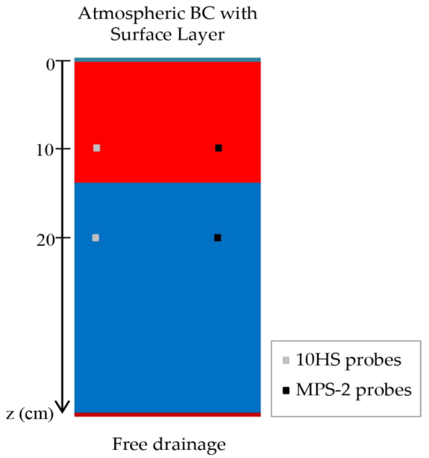
HYDRUS-1D input data components in this study include input data for the variable boundary condition (i.e., evapotranspiration, transpiration, and irrigation), soil hydraulic properties and inverse input data (soil moisture in time and retention curve data). The variable boundary condition of this study is illustrated in Figure 2.
The upper boundary condition was set to an atmospheric condition influenced by irrigation supply, and crop evapotranspiration with a surface layer as indicated in the following equation:
where is the difference between irrigation, transpiration, and evaporation rate.
The free/zero-gradient drainage boundary condition is suitable for water flow simulation of unsaturated soil in which the soil domain of interest is not affected by groundwater [86,87]. The process allows water to leave a flow domain by gravity, assuming a unit vertical hydraulic gradient without external forced drainage conditions [87]. Based on these conditions and the assumptions of no influence of the groundwater to the studied soil profile, the free drainage was considered at the bottom of the soil domain. The free drainage condition is represented as follows:
Where is the soil profile assumed at 40 cm depth.
HYDRUS-1D can give water flow at any specific soil depth [88]. The observation nodes were set at 10 and 20 cm following the location of the 10HS and MPS-2 sensors. The soil moisture at the beginning of the simulation in the soil profile domain was set to the initial observation from these 10HS sensors.
2.7. Inverse Solution
In HYDRUS-1D, the Marquart-Levenberge method is used to optimize the soil hydraulic parameters [23,90,91,92]. The optimization process to generate vG parameters by the model in this study is to minimize the difference between simulated and observed values of water content, , and soil water retention data, through an objective function, as described below [93].
where m is the two types of dataset, i.e., soil water content , and retention curve , is the number of measurements of the jth dataset, and are the observations and predictions for the jth measurement set, b (e.g., , , and ) is the vector of optimsed parameters. The first set of measurements is water content in time, using 10HS measurement, and the second is the retention curve from simultaneous measurement of 10HS soil water content and MPS-2 soil water potential. The hydraulic parameters for two soil depths at 10 and 20 cm were optimized simultaneously in the inversion process.
To evaluate the model performance, we used three fitted statistical indicators, e.g., the root mean square error (RMSE), the Nash and Sutcliffe model efficiency (NSE), and the coefficient of determination (R2) with the following expressions.
where and are the observation and simulation as described above, is total amount of the data. R2 ranges between 0 and 1. Value 1 indicates that the simulation dispersion is equal to the observation, whereas R2 equals to 0, there is no any correlation between them [94]. The lower RMSE value is, the better model performs [95]. NSE values are between −∞ and 1.0 (1 perfect fit) [95]. If 0 < NSE < 1.0, it is considered to be an acceptable performance, otherwise a negative NSE indicates unacceptable performance [95,96,97].
3. Results
3.1. Evapotranspiration Computation
3.1.1. 5-Min Timestep
Figure 3 illustrates the result of reference evapotranspiration () computed based on the Penman-Monteith equation (Equation (1)) by using meteorological data collected at 5 min resolution over the growing season from February to March 2016. 5-min between February and March ranged from 0.000143 to 0.075 mm 5-min−1, with a mean value of 0.017 mm 5-min−1 (Figure 3). The accumulative 5-min in daily estimates ranged from 4 to 6 mm day−1, which are reasonable values for this study area climate. Nobuhiro et al. [98] found that the average daily evapotranspiration levels during the late rainy season and the middle of the dry season in central Cambodia were 4.3 and 4.6 mm day−1, respectively, and the maximum daily levels were 5.2 and 5.7 mm day−1 respectively.
3.1.2. Partition of Crop Evapotranspiration
Results of estimation of transpiration and evaporation from partitioning crop evapotranspiration () based on the method proposed by Gallardo et al. [72] at sites T1, T2 and T3 are presented in Figure 4. The transpiration estimation at site T1 and T2 was done during mid-season with full canopy cover of 35% and 57% respectively and during development stage at T3 reaching the full canopy cover of 44%. The results show that soil evaporation was the main part of during the growing season. The soil evaporation ranged from 47% to 67% at the maximum canopy cover stage in the three sites.
3.2. Inversion Estimation
3.2.1. Estimated Parameters and Model Evaluation
The inverse estimation technique using HYDRUS-1D has been successfully used to determine the soil hydraulic function of van Genuchten (vG) parameters in the two soil depths of 10 cm and 20 cm in the five experimental sites. Table 6 shows the results of optimized vG parameter sets in all experimental sites. The estimated ranged from 0.35 to 0.43 cm3 cm−3 for loamy soils (T1 and T5), 0.30 to 0.35 cm3 cm−3 for sand soils (T2 and T3) and 0.32 to 0.37 cm3 cm−3 for loam soil (T4). It was noted that these estimations are similar to the measured values. At site T4, the estimated (ranging from 0.32–0.37 cm3 cm−3) is much lower than the measured value (0.43 cm3 cm−3). Commonly, the laboratory-measured can be smaller than in situ values because of incomplete saturation and air entrapment of the soil [18,99], while it is possibly over/underestimated in the laboratory-measured [100].
For the computation of saturated hydraulic conductivity parameters, it was noted that inputting low initial measured saturated conductivity in sand soil during the optimization process with = 0.43 mm min−1 at site T2 and = 1.45 mm min−1 at site T3 resulted in a divergence of the model. In that case, initial were estimated using Rosetta method of Schaap et al. [89] based on soil texture. Therefore, = 4.95 mm min−1 from Rosetta method at sites T2 and T3 was selected as the initial value and resulted in convergence. It highlights the need for reasonable input values before an inversion process.
The fitted in Table 6 were quite higher than the measured values from the tension infiltrometer (TI) in sites T1, T2, T3. The difference between in situ measured and simulated values of is most probably due to the different time and space at the measurement from the scale at which the processes are modelled [18]. It is commonly known that agricultural soils frequently exhibit extensive spatial and temporal changes in pore characteristics that cause variation change in soil hydraulic conductivity, K(h). On the other hand, it was noted that were measured by TI at the soil surface. Thus, it caused the limitation both on K(h) extrapolation towards saturation and on its application to extended depth (10 and 20 cm) [101]. Another potential reason can be due to the limitations of TI method in measurement in the coarse soil texture. The result study of March [102] suggested that TI method underestimated under high permeability conditions. Similarly, Yoon et al. [101] observed that there was greater fluctuation in measuring hydraulic conductivity near the saturated condition especially for sandy soil affected by the presence of irregular distribution of macropore possibly with entrapped air. The other limitations were described by Roulier et al. [103] mainly associated with the simplifying assumptions of the analysis methods and instrumental restriction [101]. Indeed, obtained from TI was estimated indirectly and assuming only matrix flow, that might lead to inaccurate [104].
Therefore, the inverse model estimation suggested a reasonable value of using the observed soil water dynamic. There were low estimated of coarse soils at this soil depth at site T3 at 20 cm and T5 at 10 cm. The soil compaction at 20 cm soil depth could be the reason of the low estimated permeability at site T3. It was noted that at site T5 the second soil layer below 15 cm depth was highly compacted and that could lead to the low estimation for this loamy sand at 10 cm depth. In contrast, the measured in T4 and T5 are similar to the optimized values. This suggests that a tension infiltrometer might be useful in determining for inverse estimation for fine soil type.
These results also suggest that for further work, a sensitivity analysis of the vG parameters could be interesting, to investigate the constrains of its impact on the simulation.
Table 7 and Table 8 show the evaluation model performances of the inverse estimation to generate SWRCs and water flow, respectively. After inversion, the results showed the improvement of model performance in SWRC simulation with lower RMSE (ranging from 0.01 to 0.04 cm3 cm−3) and higher coefficients of NSE (ranged from 0.53 to 0.99) and determination (R2) (ranging from 0.78 to 0.99) (Table 7). Similarly, water flow simulation resulted in satisfied performance with RMSE ranged from 0.02 to 0.03 cm3 cm−3, NSE from 0.64 to 0.83 and R2 from 0.85 to 0.99 (Table 8). Overall, these results confirm that the inverse modelling with HYDRUS-1D can predict soil water retention curve and dynamic water content in the soil profile with a reasonable degree of accuracy.
3.2.2. Soil Water Retention Curves
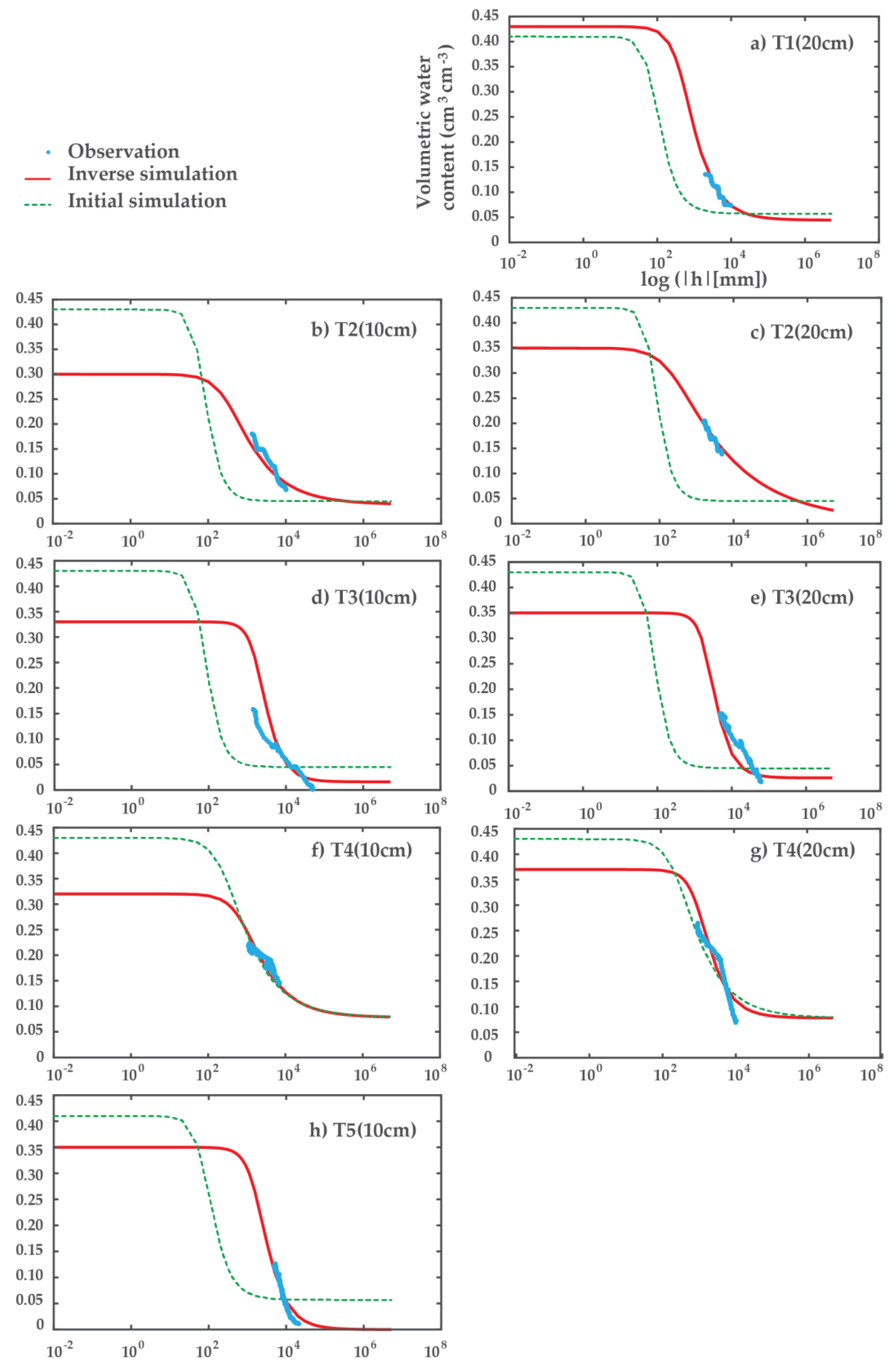
Figure 5 shows the soil water retention curves before and after inversion. Simulated SWRCs are close to the observation in all sites and depths. The excellent fits were at site T1 at 20 cm depth (loamy sand soil) (RMSE = 0.01 cm3 cm−3) and at site T2 at 20 cm depth (RMSE = 0.002 cm3 cm−3). Otherwise, the other SWRCs in the other sites and depths fitted fairly well with RMSE, ranging from 0.016 to 0.048 cm3 cm−3.
The data of field SWRC at near-saturated and driest points in all experimental sites were not presented because of data inaccuracy and limitation from the sensors (10HS and MPS-2) at these wet and dry ranges. MPS-2 is unable to provide accurate pressures at the wet end of the SWRC because of the air-entry limit [20]. The acceptable measured ranges of the sensors were selected for inverse input data as illustrated in Figure 5. Despite its limitations, MPS-2 can be useful in a drier range and to pilot irrigation [20]. Similarly, the errors from the 10HS sensor can be due to its accuracy limitations in measuring the water content in moist conditions [64]. On the other hand, the effect of temperature on the 10HS sensor response could have caused significant data errors in the fine soil and for high water content, especially at upper soil layers where there is higher temperature fluctuation [105].
The estimated AEV of the tested soils are shown in Table 6. AEV ranged from 0.86 to 12.64 kPa. AEV of loamy sand were from 2.28 to 9.60 kPa, sand were from 0.86 to 12.64 kPa, and loam were 3.37 to 5.16 kPa. Reference [106] showed that the soil with higher sand content has smaller AEV using laboratory pressure plate extractor test. They also found the effect of initial water content on the AEV. The sand soil with higher initial water content has larger AEV (i.e., the soil with sand content of 20% to 60% resulted in AEV of 6.04 to 1.94 kPa respectively). Similarly, Konyai et al. [107], using pressure plates for defining SWRCs, found the AEV of loamy sand ranged from 1.30 to 2.00 kPa and loam soil of 0.90 kPa. However, those results were from the laboratory. It is seen that the generated SWRC at site T3 with high sand content proposed a higher AEV of 10.09 and 12.64 kPa. The physical environmental effects to the SWRC of sand soil are complex in their observations at near real AEV. The limitation of sensors to catch the accuracy of the low range of suction can be the main reason for the high estimated AEV of the sand soil at T3. In Figure 5, the generated initial SWRC from the Rosetta method are often obtained from laboratory SWRC. The inverse estimated SWRC reflected the effect of the dynamic physical environmental. Therefore, it is interesting to investigate the field SWRC with the influence of the in situ environment.
3.2.3. Dynamic Soil Water Content
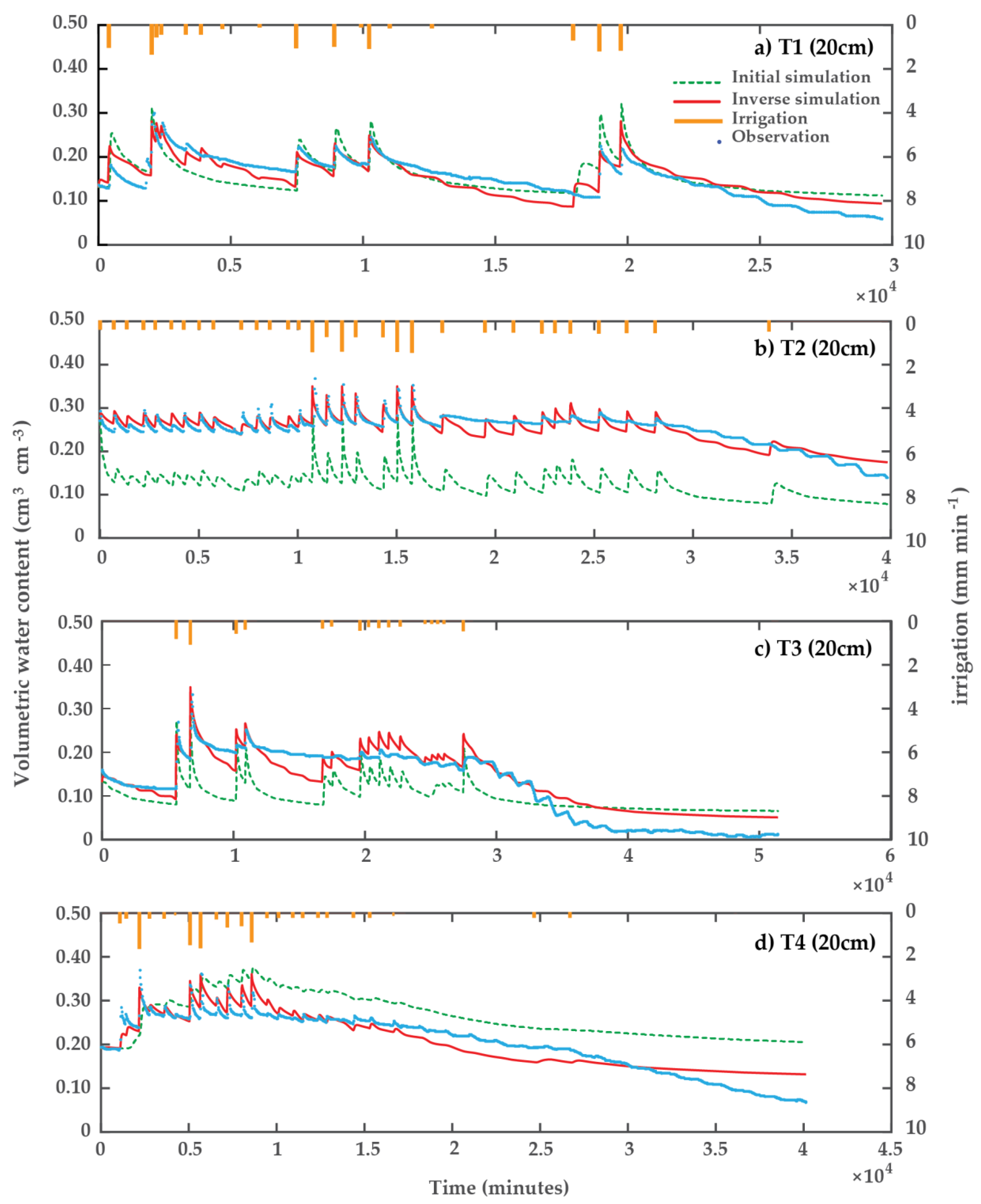
Observed and simulated soil water content distributions in the soil profile at 10 and 20 cm at the 5 experimental sites are shown in Figure 6 and Figure 7, respectively. The fluctuation of soil water content was coming from only irrigation applied at sites T1, T2, T3 and T4. The water flow simulation in all sites gave good and excellent correlations between observed and simulated water contents in the soil profile (i.e., R2 values ranged from 0.85 to 0.99). It is noted that the water flow simulation was similar to the soil moisture observation in the wet range but widely over/underestimated in the end dry events after the inversion (i.e., RMSE ranged from 0.02 to 0.03 cm3 cm−3 and NSE ranged from 0.67 to 0.84). The important factor influencing the simulation model performance is the assumption of homogeneous soil properties through the entire simulation. This assumption is not flexible to real phenomena e.g., the dynamic change of soil hydraulic properties during the growing season, the macropore flow, and lateral flux of soil moisture. Schwen et al. [2] revealed that the accuracy of the soil water flow simulation, especially of that near the surface, can be improved by using time-variable hydraulic parameters. Despite several simplifying assumptions of HYDRUS-1D model, the results of the inversion yet provided reasonable estimates of water dynamics and a better improvement from the initial simulation.
4. Conclusions
In this study, inversion approach using HYDRUS-1D based on only in situ measurement of soil hydraulic properties were used to estimate the van Genuchten (vG) parameters of the soil properties in experimental fields with different soil types including loamy sand, sand, and loam soil, in Chrey Bak Catchment, Cambodia. The in situ soil hydraulic measured data that were used as inverse input data included saturated hydraulic conductivity using tension infiltrometer, observed dynamic soil water content and SWRC from simultaneous measures of Decagon 10HS soil moisture and MPS-2 soil water potential sensors. To apply this approach, first we computed 5-min timestep reference evapotranspiration based on the ASCE Penman-Monteith equation and obtained reasonable results. Then we partitioned the crop evapotranspiration based on the Gallardo et al. [72] method in the field after lettuce was planted.
Analyzing the SWRC shows that the simulated SWRC using optimum vG parameters of the inversion closely and fairly matched the field SWRC data, with RMSE ranging from 0.002 to 0.048 cm3 cm−3. The fair match was due to the limitation in measurement of the sensors in the wet and the driest range of moisture condition in the field. In testing water flow simulation, generally the model resulted in a good simulation performance for predicting the soil water content in the experimental period in all the studied soil types, with the RMSE ranging from 0.02 to 0.03 cm3 cm−3. The results proposed that soil hydraulic properties can be estimated effectively and rapidly with inverse modelling using only the information from the field soil hydraulic measurement without the required expensive laboratory data. We found that a tension infiltrometer might be useful in determining saturated hydraulic conductivity () for inverse estimation for fine (loam) soil type, as the generated was slightly changed from the initial measured values after inversion. We confirmed that the inverse process in the model is sensitive to initial hydraulic soil parameter input, and can lead to model divergence. For further work, validation on another data set should be investigated.
It is recommended that more additional experimental data, particularly accurate field dynamic SWRC in the wet and dry encompassing new technics and methods, should be included to improve the inversion approach in further research. Additionally, the dynamic change of soil properties should be considered in the inversion model to improve the accuracy of water flow prediction.
Author Contributions
Conceptualization, Aurore Degré and Pinnara Ket; Data curation, Pinnara Ket; Investigation, Pinnara Ket; Methodology, Aurore Degré; Project administration, Chantha Oeurng and Aurore Degré; Supervision, Aurore Degré and Chantha Oeurng; Writing—original draft, Pinnara Ket; Writing—review & editing, Aurore Degré, Chantha Oeurng and Pinnara Ket.
Funding
This research was sponsored by the Belgian university cooperation programme, ARES-CCD (La Commission Coopération au Développement de l’Académie de Recherche et d’Enseignement supérieur).
Acknowledgments
The soil textures and soil pH were measured at Pedology Laboratory, Soil Science Department, Gembloux Agro Bio Tech-Liège University, Belgium. We thank the colleges for their guide and helps in the measurement.
Conflicts of Interest
The authors declare no conflict of interest.
References
- Zijlstra, J.; Dane, J.H. Identification of Hydraulic Parameters in Layered Soils Based on a Quasi-Newzon Method. J. Hydrol. 1996, 181, 233–250. [Google Scholar] [CrossRef]
- Schwen, A.; Bodner, G.; Loiskandl, W. Time-Variable Soil Hydraulic Properties in near-Surface Soil Water Simulations for Different Tillage Methods. Agric. Water Manag. 2011, 99, 42–50. [Google Scholar] [CrossRef]
- Huang, J.; Purushothaman, R.; McBratney, A.; Bramley, H. Soil Water Extraction Monitored Per Plot across a Field Experiment Using Repeated Electromagnetic Induction Surveys. Soil Syst. 2018, 2, 11. [Google Scholar] [CrossRef]
- Lai, J.; Ren, L. Estimation of Effective Hydraulic Parameters in Heterogeneous Soils at Field Scale. Geoderma 2016, 264, 28–41. [Google Scholar] [CrossRef]
- Le Bourgeois, O.; Bouvier, C.; Brunet, P.; Ayral, P.A. Inverse Modeling of Soil Water Content to Estimate the Hydraulic Properties of a Shallow Soil and the Associated Weathered Bedrock. J. Hydrol. 2016, 541, 116–126. [Google Scholar] [CrossRef]
- Vereecken, H.; Schnepf, A.; Hopmans, J.W.; Javaux, M.; Or, D.; Roose, T.; Vanderborght, J.; Young, M.H.; Amelung, W.; Aitkenhead, M.; et al. Modeling Soil Processes: Review, Key Challenges, and New Perspectives. Vadose Zone J. 2016, 15, 1–57. [Google Scholar] [CrossRef] [Green Version]
- Peters, A.; Durner, W. Simplified Evaporation Method for Determining Soil Hydraulic Properties. J. Hydrol. 2008, 356, 147–162. [Google Scholar] [CrossRef]
- Moret-Fernández, D.; Latorre, B. Estimate of the Soil Water Retention Curve from the Sorptivity and β Parameter Calculated from an Upward Infiltration Experiment. J. Hydrol. 2017, 544, 352–362. [Google Scholar] [CrossRef]
- Hopmans, J.; Simunek, J. Review of Inverse Estimation of Soil Hydraulic Properties. In Characterization and Measurement of the Hydraulic Properties of Unsaturated Porous Media; van Genuchten, M.T., Leij, F.J., Eds.; University of California: Riverside, CA, USA, 1999; pp. 643–659. [Google Scholar]
- Gupta, S.C.; Larson, W.E. Estimating Soil Water Retention Characteristics from Particle Size Distribution, Organic Matter Percent, and Bulk Density. Water Resour. Res. 1979, 15, 1633–1635. [Google Scholar] [CrossRef]
- Botula, Y.D.; Van Ranst, E.; Cornelis, W.M. Pedotransfer Functions to Predict Water Retention for Soils of the Humid Tropics: A Review. Rev. Bras. Cienc. Solo 2014, 38, 679–698. [Google Scholar] [CrossRef]
- Rashid, N.S.A.; Askari, M.; Tanaka, T.; Simunek, J.; van Genuchten, M.T. Inverse Estimation of Soil Hydraulic Properties under Oil Palm Trees. Geoderma 2015, 241–242, 306–312. [Google Scholar] [CrossRef]
- Smagin, A.V. Column-Centrifugation Method for Determining Water Retention Curves of Soils and Disperse Sediments. Eurasian Soil Sci. 2012, 45, 416–422. [Google Scholar] [CrossRef]
- Ramos, T.B.; Gonçalves, M.C.; Martins, J.C.; van Genuchten, M.T.; Pires, F.P. Estimation of Soil Hydraulic Properties from Numerical Inversion of Tension Disk Infiltrometer Data. Vadose Zone J. 2006, 5, 684–696. [Google Scholar] [CrossRef]
- Schwartz, R.C.; Evett, S.R. Estimating Hydraulic Properties of a Fine-Textured Soil Using a Disc Infiltrometer. Soil Sci. Soc. Am. J. 2002, 66, 1409–1423. [Google Scholar] [CrossRef]
- Ventrella, D.; Losavio, N.; Vonella, A.V.; Leij, F.J. Estimating Hydraulic Conductivity of a Fine-Textured Soil Using Tension Infiltrometry. Geoderma 2005, 124, 267–277. [Google Scholar] [CrossRef]
- Lazarovitch, N.; Ben-Gal, A.; Šimunek, J.; Shani, U. Uniqueness of Soil Hydraulic Parameters Determined by a Combined Wooding Inverse Approach. Soil Sci. Soc. Am. J. 2007, 71, 860–865. [Google Scholar] [CrossRef]
- Verbist, K.; Cornelis, W.M.; Gabriels, D.; Alaerts, K.; Soto, G.; Serena, L. Using an Inverse Modelling Approach to Evaluate the Water Retention in a Simple Water Harvesting Technique. Hydrol. Earth Syst. Sci. 2009, 13, 1979–1992. [Google Scholar] [CrossRef]
- Latorre, B.; Moret-Fernández, D.; Peña, C. Estimate of Soil Hydraulic Properties from Disc Infiltrometer Three-Dimensional Infiltration Curve: Theoretical Analysis and Field Applicability. Procedia Environ. Sci. 2013, 19, 580–589. [Google Scholar] [CrossRef]
- Degré, A.; van der Ploeg, M.; Caldwell, T.M.; Gooren, H. Comparison of Soil Water Potential Sensors: A Drying Experiment. Vadose Zone J. 2017, 16, 4. [Google Scholar] [CrossRef]
- Asgarzadeh, H.; Mosaddeghi, M.R.; Dexter, A.R.; Mahboubi, A.A.; Neyshabouri, M.R. Determination of Soil Available Water for Plants: Consistency between Laboratory and Field Measurements. Geoderma 2014, 226–227, 8–20. [Google Scholar] [CrossRef]
- Li, Y.B.; Liu, Y.; Nie, W.B.; Ma, X.Y. Inverse Modeling of Soil Hydraulic Parameters Based on a Hybrid of Vector-Evaluated Genetic Algorithm and Particle Swarm Optimization. Water 2018, 10, 84. [Google Scholar] [CrossRef]
- Wang, T.; Franz, T.E.; Yue, W.; Szilagyi, J.; Zlotnik, V.A.; You, J.; Chen, X.; Shulski, M.D.; Young, A. Feasibility Analysis of Using Inverse Modeling for Estimating Natural Groundwater Recharge from a Large-Scale Soil Moisture Monitoring Network. J. Hydrol. 2016, 533, 250–265. [Google Scholar] [CrossRef]
- Van den Berg, M.; Klamt, E.; Van Reeuwijk, L.P. Pedotransfer Functions for the Estimation of Moisture Retention Characteristics of Ferralsols and Related Soils. Geoderma 1997, 78, 161–180. [Google Scholar] [CrossRef]
- Werisch, S.; Grundmann, J.; Al-Dhuhli, H.; Algharibi, E.; Lennartz, F. Multiobjective Parameter Estimation of Hydraulic Properties for a Sandy Soil in Oman. Environ. Earth Sci. 2014, 72, 4935–4956. [Google Scholar] [CrossRef]
- Abbaspour, K.C.; Schulin, R.; Van Genuchten, M.T. Estimating Unsaturated Soil Hydraulic Parameters Using Ant Colony Optimization. Adv. Water Resour. 2001, 24, 827–841. [Google Scholar] [CrossRef]
- Wohling, T.; Vrugt, J.A.; Barkle, G.F. Comparison of Three Multiobjective Optimization Algorithms for Inverse Modeling of Vadose Zone Hydraulic Properties. Soil Sci. Soc. Am. J. 2008, 72, 305–319. [Google Scholar] [CrossRef]
- Kumar, S.; Sekhar, M.; Reddy, D.V.; Mohan Kumar, M.S. Estimation of Soil Hydraulic Properties and Their Uncertainty: Comparison between Laboratory and Field Experiment. Hydrol. Process. 2010, 24, 3426–3435. [Google Scholar] [CrossRef]
- Osorio-Murillo, C.A.; Over, M.W.; Savoy, H.; Ames, D.P.; Rubin, Y. Software Framework for Inverse Modeling and Uncertainty Characterization. Environ. Model. Softw. 2015, 66, 98–109. [Google Scholar] [CrossRef]
- Van Dam, J.C.; Stricker, J.N.M.; Droogers, P. Inverse Method for Determining Soil Hydraulic Functions from One-Step Outflow Experiments. Soil Sci. Soc. Am. J. 1992, 56, 1042–1050. [Google Scholar] [CrossRef]
- Gardner, W.R. Some Steady-State Solutions of the Unsaturated Moisture Flow Equation with Application to Evaporation from a Water Table. Soil Sci. 1958, 85, 228–232. [Google Scholar] [CrossRef]
- Durner, W. Hydraulic Conductivity Estimation for Soils with Heterogeneous Pore Structure. Water Resour. Res. 1994, 30, 211–223. [Google Scholar] [CrossRef]
- Campbell, G. A Simple Method for Determining Unsaturated Conductivity from Moisture Retention Data. Soil Sci. 1974, 117, 311–314. [Google Scholar] [CrossRef]
- Van Genuchten, M.T. A Closed-Form Equation for Predicting the Hydraulic Conductivity of Unsaturated Soils. Soil Sci. Soc. Am. J. 1980, 44, 892–898. [Google Scholar] [CrossRef]
- Lambot, S. A Global Multilevel Coordinate Search Procedure for Estimating the Unsaturated Soil Hydraulic Properties. Water Resour. Res. 2002, 38, 1–15. [Google Scholar] [CrossRef]
- Fuentes, C.; Haverkamp, R.; Parlange, J.Y. Parameter Constraints on Closed-Form Soil Water Relationships. J. Hydrol. 1992, 134, 117–142. [Google Scholar] [CrossRef]
- Shi, L.; Song, X.; Tong, J.; Zhu, Y.; Zhang, Q. Impacts of Different Types of Measurements on Estimating Unsaturated Flow Parameters. J. Hydrol. 2015, 524, 549–561. [Google Scholar] [CrossRef]
- Kool, J.B.; Parker, J.C.; Van Genuchten, M.T. Determining Soil Hydraulic Properties from One-Step Outflow Experiments by Parameter Estimation: I. Theory and Numerical Studies. Soil Sci. Soc. Am. J. 1985, 49, 1348–1354. [Google Scholar] [CrossRef]
- Toorman, A.F.; Wierenga, P.J.; Hills, R.G. Parameter Estimation of Hydraulic Properties from One-step Outflow Data. Water Resour. Res. 1992, 28, 3021–3028. [Google Scholar] [CrossRef]
- Eching, S.O.; Hopmans, J.W. Optimization of Hydraulic Functions from Transient Outflow and Soil Water Pressure Data. Soil Sci. Soc. Am. J. 1993, 57, 1167–1175. [Google Scholar] [CrossRef]
- Simůnek, J.; van Genuchten, M.T. Estimating Unsaturated Soil Hydraulic Properties from Multiple Tension Disc Infiltrometer Data. Soil Sci. 1997, 162, 383–398. [Google Scholar] [CrossRef]
- Schelle, H.; Durner, W.; Iden, S.C.; Fank, J. Simultaneous Estimation of Soil Hydraulic and Root Distribution Parameters from Lysimeter Data by Inverse Modeling. Procedia Environ. Sci. 2013, 19, 564–573. [Google Scholar] [CrossRef]
- Kechavarzi, C.; Špongrová, K.; Dresser, M.; Matula, S.; Godwin, R.J. Laboratory and Field Testing of an Automated Tension Infiltrometer. Biosyst. Eng. 2009, 104, 266–277. [Google Scholar] [CrossRef]
- Wayllace, A.; Lu, N. A Transient Water Release and Imbibitions Method for Rapidly Measuring Wetting and Drying Soil Water Retention and Hydraulic Conductivity Functions. Geotech. Test. J. 2011, 35, 103–117. [Google Scholar]
- Wang, J.E.; Xiang, W. Transient Water Release and Imbibition Properties of Remolded Sliding Zone Soil of Huangtupo Landslide in Three Gorges Reservoir Area, China. In Global View of Engineering Geology and the Environment, Proceedings of the International Symposium and 9th Asian Regional Conference of IAEG, Beijing, China, 23–25 September 2013; CRC Press: London, UK, 2014; p. 228. [Google Scholar]
- Lu, N. Validating the Effective Stress Principle in Unsaturated Soil Using Non-Failure Tests. In Unsaturated Soils: Research & Applications; Khalili, N., Russell, A., Khoshghalb, A., Eds.; CRC Press: London, UK, 2014; pp. 31–41. [Google Scholar]
- Mun, W.; Teixeira, T.; Balci, M.C.; Svoboda, J.; Mccartney, J.S. Rate Effects on the Undrained Shear Strength of Compacted Clay. Soil Found. 2016, 56, 719–731. [Google Scholar] [CrossRef]
- Lu, N.; Wayllace, A.; Oh, S. Infiltration-Induced Seasonally Reactivated Instability of a Highway Embankment near the Eisenhower Tunnel, Colorado, USA. Eng. Geol. 2013, 162, 22–32. [Google Scholar] [CrossRef]
- Lu, N.; Godt, J.W. Hillslope Hydrology and Stability; Cambridge University Press: Cambridge, UK, 2013. [Google Scholar]
- Ritter, A.; Hupet, F.; Munoz-Carpena, R.; Lambot, S.; Vanclooster, M. Using Inverse Methods for Estimating Soil Hydraulic Properties from Field Data as an Alternative to Direct Methods. Agric. Water Manag. 2003, 59, 77–96. [Google Scholar] [CrossRef]
- Köhne, J.M.; Köhne, S.; Šimůnek, J. A Review of Model Applications for Structured Soils: A) Water Flow and Tracer Transport. J. Contam. Hydrol. 2009, 104, 4–35. [Google Scholar] [CrossRef] [PubMed]
- Filipović, V.; Weninger, T.; Filipović, L.; Schwen, A.; Bristow, K.L.; Zechmeister-Boltenstern, S.; Leitner, S. Inverse Estimation of Soil Hydraulic Properties and Water Repellency Following Artificially Induced Drought Stress. J. Hydrol. Hydromech. 2018, 66, 170–180. [Google Scholar] [CrossRef]
- Chann, S.; Wales, N.; Frewer, T. An Investigation of Land Cover and Land Use Change in Stung Chrey Bak Catchment, Cambodia; CDRI: Phnom Penh, Cambodia, 2011. [Google Scholar]
- FAO (Food and Agriculture Organization of the United Nations). Guidelines for Soil Description, 4th, ed.; Food and Agriculture Organization of the United Nations: Rome, Italy, 2006. [Google Scholar]
- Ket, P.; Garré, S.; Oeurng, C.; Hok, L.; Degré, A. Simulation of Crop Growth and Water-Saving Irrigation Scenarios for Lettuce: A Monsoon-Climate Case Study in Kampong Chhnang, Cambodia. Water 2018, 10, 666. [Google Scholar] [CrossRef]
- Andersland, O.B.; Ladanyi, B. Frozen Ground Engineering, 3rd, ed.; John Wiley & Sons: Hoboken, NJ, USA, 2004. [Google Scholar]
- Liénard, A.; Colinet, G. Transfert En Cadmium et Zinc Vers l ’orge de Printemps En Sols Contaminés et Non Contaminés de Belgique: Évaluation et Prédiction. Cah. Agric 2018, 27, 1–10. [Google Scholar] [CrossRef]
- Wooding, R.A. Steady Infiltration from a Shallow Circular Pond. Water Resour. Res. 1968, 4, 1259–1273. [Google Scholar] [CrossRef]
- Fisher, D.K.; Gould, P.J. Open-Source Hardware Is a Low-Cost Alternative for Scientific Instrumentation and Research. Mod. Instrum. 2012, 1, 8–20. [Google Scholar] [CrossRef]
- Decagon Devices. MPS-2 & MPS-6 Dielectric Water Potential Sensors, Operator’s Manual; Decagon Devices, Inc.: Pullman, WA, USA, 2016. [Google Scholar]
- Decagon Devices. MPS-2 Dielectric Water Potential Sensor: Operator’s Manual; Decagon Devices, Inc.: Pullman, WA, USA, 2011. [Google Scholar]
- Decagon Devices. 10HS Soil Moisture Sensor Operator’s Manual; Version 3; Decagon Devices, Inc.: Pullman, WA, USA, 2010. [Google Scholar]
- Visconti, F.; de Paz, J.M.; Martínez, D.; Molina, M.J. Laboratory and Field Assessment of the Capacitance Sensors Decagon 10HS and 5TE for Estimating the Water Content of Irrigated Soils. Agric. Water Manag. 2014, 132, 111–119. [Google Scholar] [CrossRef]
- Mittelbach, H.; Lehner, I.; Seneviratne, S.I. Comparison of Four Soil Moisture Sensor Types under Field Conditions in Switzerland. J. Hydrol. 2012, 430–431, 39–49. [Google Scholar] [CrossRef]
- Cobos, D.; Chamber, C. Application Note Calibrating ECH2O Soil Moisture Sensors; Decagon Devices, Inc.: Pullman, WA, USA, 2005; pp. 1–5. [Google Scholar]
- Irmak, S.; Howell, T.A.; Allen, R.G.; Payero, J.O.; Martin, D.L. Standardized ASCE Penman-Monteith: Impact of Sum-of-Hourly vs. 24-Hour Timestep Computations at Reference Weather Station Sites. Trans. ASAE 2005, 48, 1063–1077. [Google Scholar] [CrossRef]
- Allen, R.; Walter, I.; Elliott, R. The ASCE Standardized Reference Evapotranspiration Equation; American Society of Civil Engineers: Reston, VA, USA, 2005. [Google Scholar]
- Allen, R.G.; Pruitt, W.O.; Wright, J.L.; Howell, T.A.; Ventura, F.; Snyder, R.; Itenfisu, D.; Steduto, P.; Berengena, J.; Baselga, J.; et al. A Recommendation on Standardized Surface Resistance for Hourly Calculation of Reference ETo by the FAO56 Penman-Monteith Method. Agric. Water Manag. 2006, 81, 1–22. [Google Scholar] [CrossRef]
- Tolk, J.A.; Evett, S.R.; Schwartz, R.C. Field-Measured, Hourly Soil Water Evaporation Stages in Relation to Reference Evapotranspiration Rate and Soil to Air Temperature Ratio. Vadose Zone J. 2015, 14, 1–14. [Google Scholar] [CrossRef]
- Kool, D.; Agam, N.; Lazarovitch, N.; Heitman, J.L.; Sauer, T.J.; Ben-gal, A. A Review of Approaches for Evapotranspiration Partitioning. Agric. For. Meteorol. 2014, 184, 56–70. [Google Scholar] [CrossRef]
- Paredes, P.; Rodrigues, G.C.; Alves, I.; Pereira, L.S. Partitioning Evapotranspiration, Yield Prediction and Economic Returns of Maize under Various Irrigation Management Strategies. Agric. Water Manag. 2014, 135, 27–39. [Google Scholar] [CrossRef]
- Gallardo, M.; Snyder, R.; Schulbach, K.; Jackson, L. Crop Growth and Water Use Model for Lettuce. J. Irrig. Drain. Eng. 1996, 122, 354–359. [Google Scholar] [CrossRef]
- Doorenbos, J.; Pruitt, W.O. Guidelines for Predicting Crop Water Requirements; Food and Agriculture Organization of the United Nations: Rome, Italy, 1977. [Google Scholar]
- Šimůnek, J.; Šejna, M.; Saito, H.; Sakai, M.; Van Genuchten, M. The HYDRUS-1D Software Package for Simulating the One-Dimensional Movement of Water Heat, and Multiple Solutes in Variably-Saturated Media; Department of Environmental Sciences, University of California: Riverside, CA, USA, 2005. [Google Scholar]
- May, P.; Genuchten, V. Modeling Nonequilibrium Flow and Transport Processes Using HYDRUS. Vadose Zone J. 2008, 7, 782–797. [Google Scholar]
- Richards, L.A. Capillary Conduction of Liquids Throuhg Porous Media. Physics 1931, 1, 318–333. [Google Scholar] [CrossRef]
- Mualem, Y. A New Model for Predicting the Hydraulic Conductivity of Unsaturated Porous Media. Water Resour. Res. 1976, 12, 513–522. [Google Scholar] [CrossRef]
- Šimůnek, J.; Jarvis, N.J.; van Genuchten, M.T.; Gärdenäs, A. Review and Comparison of Models for Describing Non-Equilibrium and Preferential Flow and Transport in the Vadose Zone. J. Hydrol. 2003, 272, 14–35. [Google Scholar] [CrossRef]
- Radcliffe, D.E.; Simunek, J. Soil Physics with Hydrus Modeling and Applications; CRC Press, Taylor and Francis Group, LLC: Boca Raton, FL, USA, 2010. [Google Scholar]
- Soltani, A.; Azimi, M.; Deng, A.; Taheri, A. A Simplified Method for Determination of the Soil—Water Characteristic Curve Variables. Int. J. Geotech. Eng. 2017, 1–10. [Google Scholar] [CrossRef]
- Zhai, Q.; Rahardjo, H. Quanti Fi Cation of Uncertainties in Soil—Water Characteristic Curve Associated with Fi Tting Parameters. Eng. Geol. 2013, 163, 144–152. [Google Scholar] [CrossRef]
- Barbour, S.L. Nineteenth Canadian Geotechnical Colloquium: The Soil-Water Characteristic Curve: A Historical Perspective. Can. J. Geotech 1998, 35, 873–894. [Google Scholar] [CrossRef]
- Assouline, S.; Tessier, D. A Conceptual Model of the Soil Water Retention Curve. Water Resour. Res 1998, 34, 223–231. [Google Scholar] [CrossRef]
- Gallage, C.P.K.; Uchimura, T. Effects of Dry Density and Grain Size Distribution on Soil-Water Characteristic Curves of Sandy Soils. Soil Found. 2010, 50, 161–172. [Google Scholar] [CrossRef]
- Wang, Z.; Wu, L.; Wu, Q.J. Water-Entry Value as an Alternative Indicator of Soil Water-Repellency and Wettability. J. Hydrol. 2000, 231–232, 76–83. [Google Scholar] [CrossRef]
- Seki, K.; Ackerer, P.; Lehmann, F. Geoderma Sequential Estimation of Hydraulic Parameters in Layered Soil Using Limited Data. Geoderma 2015, 247–248, 117–128. [Google Scholar] [CrossRef]
- Yates, M.V. Measurement of Virus and Indicator Survival and Transport in the Subsurface; American Water Works Association: Denver, CO, USA, 2000. [Google Scholar]
- Mazzacavallo, M.G.; Kulmatiski, A. Modelling Water Uptake Provides a New Perspective on Grass and Tree Coexistence. PLoS ONE 2015, 10, e0144300. [Google Scholar] [CrossRef] [PubMed]
- Schaap, M.G.; Leij, F.J.; Van Genuchten, M.T. Rosetta: A Computer Program for Estimating Soil Hydraulic Parameters with Hierarchical Pedotransfer Functions. J. Hydrol. 2001, 251, 163–176. [Google Scholar] [CrossRef]
- Gutmann, E.D.; Small, E.E. A Comparison of Land Surface Model Soil Hydraulic Properties Estimated by Inverse Modeling and Pedotransfer Functions. Water Resour. Res. 2007, 43, 1–13. [Google Scholar] [CrossRef]
- Levenberg, K. A Method for the Solution of Certain Problems in Leaset Squares. Q. Appl. Math. 1944, 2, 164–168. [Google Scholar] [CrossRef]
- Vrugt, J.A.; van Wijk, M.T.; Hopmans, J.W. One-, Two-, and Three-Dimensional Root Water Uptake Functions for Transient Modeling. Water Resour. Res 2001, 37, 2457–2470. [Google Scholar] [CrossRef]
- Šimůnek, J.; van Genuchten, M.T.; Wendroth, O. Parameter Estimation Analysis of the Evaporation Method for Determining Soil Hydraulic Properties. Soil Sci. Soc. Am. J. 1998, 62, 894–905. [Google Scholar] [CrossRef]
- Krause, P.; Boyle, D.P. Comparison of Different Efficiency Criteria for Hydrological Model Assessment. Adv. Geosci. 2005, 5, 89–97. [Google Scholar] [CrossRef]
- Moriasi, D.N.; Arnold, J.G.; Van Liew, M.W.; Bingner, R.L.; Harmel, R.D.; Veith, T.L. Model Evaluation Quidelines for Systematic Quantification of Accuracy in Watershed Simulations. Trans. ASABE 2007, 50, 885–900. [Google Scholar] [CrossRef]
- Autovino, D.; Rallo, G.; Provenzano, G. Predicting Soil and Plant Water Status Dynamic in Olive Orchards under Different Irrigation Systems with Hydrus-2D: Model Performance and Scenario Analysis. Agric. Water Manag. 2018, 203, 225–235. [Google Scholar] [CrossRef]
- Jiang, J.; Feng, S.; Ma, J.; Huo, Z.; Zhang, C. Field Crops Research Irrigation Management for Spring Maize Grown on Saline Soil Based on SWAP Model. F. Crop. Res. 2016, 196, 85–97. [Google Scholar] [CrossRef]
- Nobuhiro, T.; Shimizu, A.; Kabeya, N.; Tamai, K.; Ito, E.; Araki, M.; Kubota, T.; Tsuboyama, Y.; Chann, S. Advanced Bash-Scripting Guide An in-Depth Exploration of the Art of Shell Scripting Table of Contents. Hydrol. Process. 2010, 22, 2267–2274. [Google Scholar]
- Schwartz, R.C.; Evett, S.R. Conjunctive Use of Tension Infiltrometry and Time-Domain Reflectometry for Inverse Estimation of Soil Hydraulic Properties. Vadose Zone J. 2003, 2, 530–538. [Google Scholar] [CrossRef]
- Abbasi, F.; Simunek, J.; Feyen, J.; Shouse, P.J. Simulataneous Inverse Estimation of Soil Hydraulic and Solute Transport Parameters from Transient Field Experiments: Homogeneous Soil. Am. Soc. Agric. Eng. 2003, 46, 1085–1095. [Google Scholar]
- Yoon, Y.; Kim, J.; Hyun, S. Estimating Soil Water Retention in a Selected Range of Soil Pores Using Tension Disc Infiltrometer Data. Soil Tillage Res. 2007, 97, 107–116. [Google Scholar] [CrossRef]
- March, P. Comparison of Tension Infiltrometer, Pressure Infiltrometer, and Soil Core Estimates of Saturated Hydraulic Conductivity. Soil Sci. Soc. Am. J. 2000, 64, 478–484. [Google Scholar]
- Roulier, Â.; Angulo-jaramillo, R.; Vandervaere, J.; Thony, J.; Gaudet, J.; Vauclin, M. Field Measurement of Soil Surface Hydraulic Properties by Disc and Ring Infiltrometers: A Review and Recent Developments. Soil Tillage Res. 2000, 55, 1–29. [Google Scholar]
- Rezaei, M.; Seuntjens, P.; Shahidi, R.; Joris, I.; Boënne, W.; Al-barri, B.; Cornelis, W. The Relevance of In-Situ and Laboratory Characterization of Sandy Soil Hydraulic Properties for Soil Water Simulations. J. Hydrol. 2016, 534, 251–265. [Google Scholar] [CrossRef]
- Kargas, G.; Soulis, K. Performance Analysis and Calibration of a New Low-Cost Capacitance Soil Moisture Sensor. J. Irrig. Drain. Eng. 2011, 138, 632–641. [Google Scholar] [CrossRef]
- Hao, D.R.; Liao, H.J.; Ning, C.M.; Shan, X.P. The Microstructure and Soil-Water Characteristic of Unsaturated Loess. In Unsaturated Soil Mechanics—From Theory to Practice, Proceedings of the 6th Asia Pacific Conference on Unsaturated Soils, Guilin, China, 23–26 October 2015; Taylor & Francis Group: London, UK, 2015; pp. 163–167. [Google Scholar]
- Konyai, S.; Sriboonlue, V.; Trelo-Ges, V. The Effect of Air Entry Values on Hysteresis of Water Retention Curve in Saline Soil. Am. J. Environ. Sci. 2009, 5, 341–345. [Google Scholar] [CrossRef]
Figure 1.
Map of experimental sites.
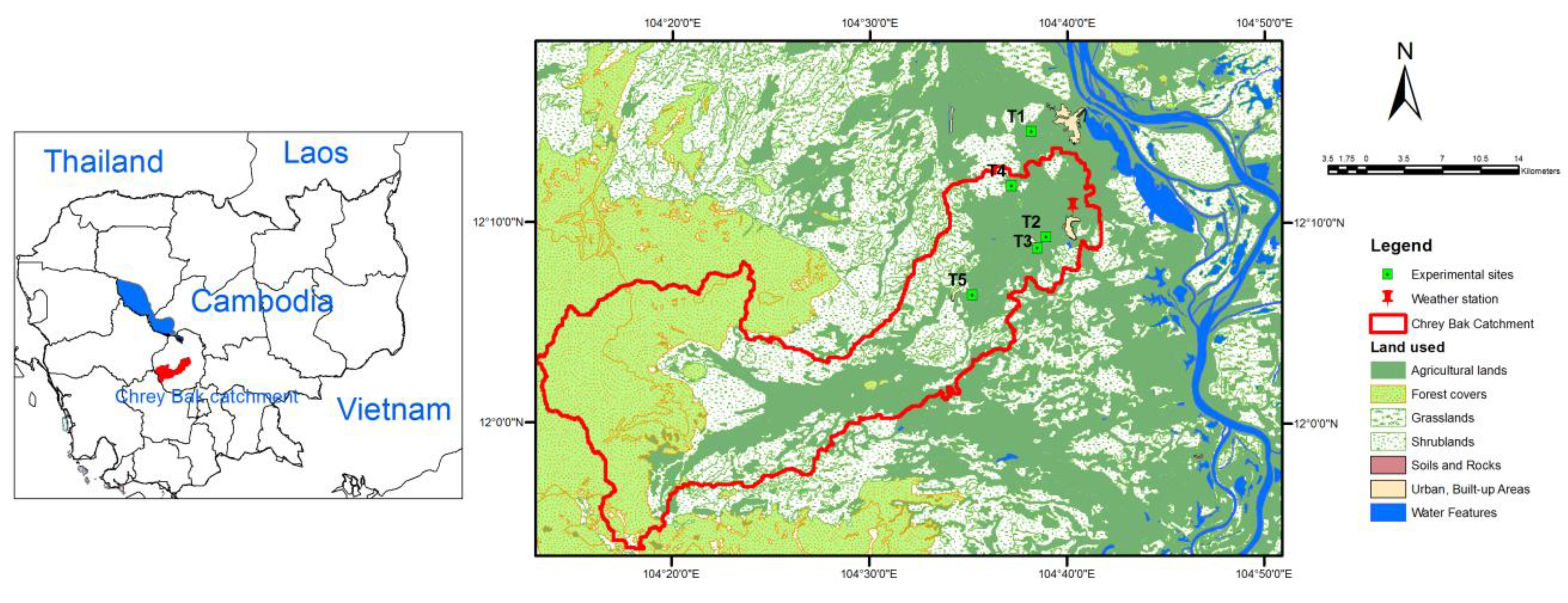
Figure 2.
Scheme of boundary condition of HYDRUS in present study.

Figure 3.
5-min timestep reference evapotranspiration during growing season in 2016, estimated based on standardized ASCE Penman-Monteith approach.
Figure 3.
5-min timestep reference evapotranspiration during growing season in 2016, estimated based on standardized ASCE Penman-Monteith approach.
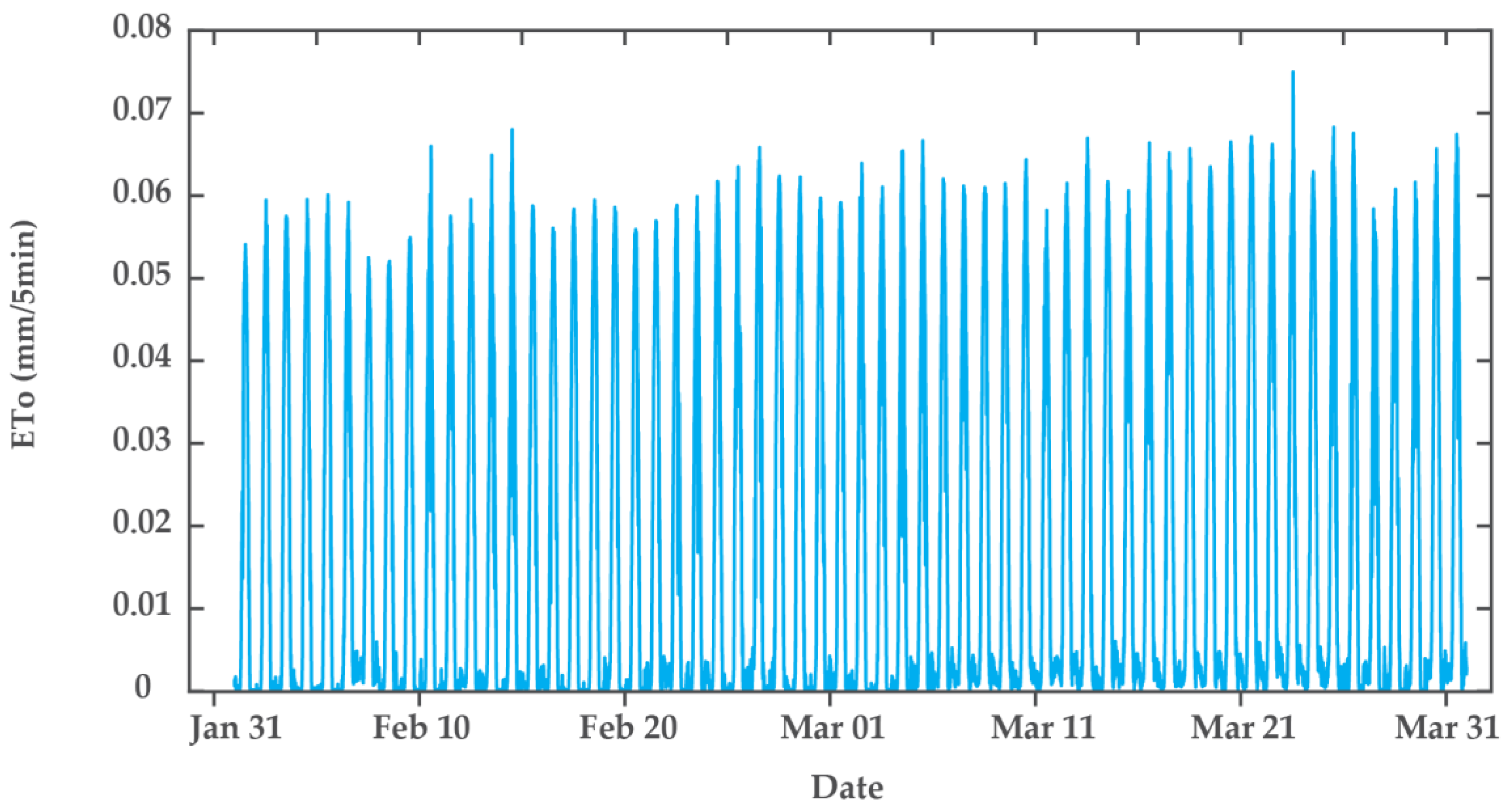
Figure 4.
Partitioning crop evapotranspiration. ET is crop evapotranspiration, E is evaporation, T is crop transpiration, (a) at site T1; (b) at site T2; (c) at site T3.
Figure 4.
Partitioning crop evapotranspiration. ET is crop evapotranspiration, E is evaporation, T is crop transpiration, (a) at site T1; (b) at site T2; (c) at site T3.

Figure 5.
SWRC in before and after inversion solution. (a) SWRC at 20 cm depth at site T1; (b) SWRC at 10 cm depth at site T2; (c) SWRC at 20 cm depth at site T2; (d) SWRC at 10 cm depth at site T3, (e) SWRC at 20 cm depth at site T3; (f) SWRC at 10 cm depth at site T4; (g) SWRC at 20 cm depth at site T4; (h) SWRC at 10 cm depth at site T5. The measured soil water potential (h) ranged from −20 to −95 kPa at site T1, from −13 to −99 kPa and −15 to −48 kPa at soil depth of 10 and 20 cm respectively at site T2, from −14 to −476 kPa and −48 to −608 kPa at 10 and 20 cm respectively at site T3, from −11 to −69 and −10 to −111 kPa at 10 and 20 cm respectively at T4, from −48 to −212 kPa at 10 cm at site T5.

Figure 6.
Observed and simulated dynamic soil moisture in 30-min timestep using inversion approach during the growing season in 2016 at different sites at 10 cm depth. (a) at site T1; (b) at site T2; (c) at site T3; (d) at site T4; (e) at site T5.
Figure 6.
Observed and simulated dynamic soil moisture in 30-min timestep using inversion approach during the growing season in 2016 at different sites at 10 cm depth. (a) at site T1; (b) at site T2; (c) at site T3; (d) at site T4; (e) at site T5.

Figure 7.
Observed and simulated dynamic soil moisture in 30-min timestep using inversion approach during the growing season in 2016 at different sites at 20 cm depth. (a) at site T1; (b) at site T2; (c) at site T3; (d) at site T4.
Figure 7.
Observed and simulated dynamic soil moisture in 30-min timestep using inversion approach during the growing season in 2016 at different sites at 20 cm depth. (a) at site T1; (b) at site T2; (c) at site T3; (d) at site T4.

Table 1.
Soil description of the study sites.
| Sites | Soil FAO Description |
|---|---|
| T1 (104°38′13.539″ E 12°14′33.951″ N, PreyMorn Village) | Horizon1 (Ap): Depth: 0–20 cm, texture: loamy sand, structure: blocky subangular, soil color: 10YR3/3, consistency of soil when dry: very friable, soil stickiness: slightly sticky, soil plasticity: slightly plastic, bulk density: 1.4–1.6 kg dm−3. Horizon2 (B1): Depth: 20–50 cm, texture: loamy sand, structure: blocky subangular, soil color: 7.5YR7/6, consistency of soil when dry: very friable, soil stickiness: non-sticky, soil plasticity: non-plastic, bulk density: 1.4–1.6 kg dm−3. Horizon 3 (B2): Depth: 50 cm+, texture: loamy sand, structure: Single grain, soil color: 7.5YR7/8, consistency of soil when dry: very friable, soil stickiness: non-sticky, soil plasticity: non-plastic, bulk density: 1.4–1.6 kg dm−3. |
| T2 (104°38′54.442″ E 12°9′15.482″ N, Chea Rov Village) | Horizon1 (Ap1): Depth: 0–10 cm, texture: sand, structure: single grain, soil color: 7.5YR5/3, consistency of soil when dry: loose, soil stickiness: slightly sticky, soil plasticity: slightly plastic, bulk density: 0.9–1.2 kg dm−3. Horizon2 (Ap2): Depth: 10–40 cm, texture: sand, structure: single grain and subangular, soil color: 7.5YR7/3, consistency of soil when dry: loose, soil stickiness: slightly sticky, soil plasticity: slightly plastic, bulk density: 1.2–1.4 kg dm−3. Horizon3 (B): Depth: 40 cm+, texture: sand, structure: single grain and subangular, soil color: 7.5Y5/4, consistency of soil when dry: loose, soil stickiness: slightly sticky, soil plasticity: slightly plastic, bulk density: 1.2–1.4 kg dm−3. |
| T3 (104°38′35.317″ E 12°8′41.929″ N, Trapain Trach village) | Horizon1 (Ap): Depth: 0–20 cm, texture: sand, structure: single grain to subangular, soil color: 7.5YR5/6, consistency of soil when dry: loose, soil stickiness: slightly sticky, soil plasticity: slightly plastic, bulk density 1.2–1.4 kg dm−3. Horizon2 (B): Depth: 20–60 cm, texture: sand, structure: single grain to subangular, soil color: 7.5YR5/6, consistency of soil when dry: loose, soil stickiness: slightly sticky, soil plasticity: slightly plastic, bulk density 1.2–1.4 kg dm−3. Horizon3 (C): Depth: 60 cm+: Bed rock. |
| T4 (104°37′16.24″ E 12°11′52.518″ N, Ou Roung Village) | Horizon1 (Ap1): Depth: 4–17 cm, texture: loam, structure: subangular, soil color: 7.5YR5/3, consistency of soil when dry: hard, soil stickiness: sticky, soil plasticity: plastic, bulk density: 1.4–1.6 kg dm−3. Horizon2 (A2): Depth: 10–40 cm, texture: loam, structure: massive subangular, soil color: 7.5YR6/3, consistency of soil when dry: very hard, soil stickiness: very sticky, soil plasticity: very plastic, bulk density: 1.0–1.2 kg dm−3. Horizon 3 (B): Depth: 17 cm+, texture: silty clay, structure: massive subangular, soil color: 7.5YR7/3, consistency of soil when dry: extremely hard, soil stickiness: very sticky, soil plasticity: very plastic, bulk density: 1.0–1.2 kg dm−3. |
| T5 (104°35′15.321″ E 12°6′21.25″ N, Kouk Pouch Village) | Horizon1 (Ap): Depth: 0–30 cm, texture: loamy sand, structure: single grain to subangular, soil color: 7.5YR5/4, consistency of soil when dry: soft, soil stickiness: slightly sticky, soil plasticity: slightly plastic, bulk density: 0.9–1.2 kg dm−3. Horizon2 (B): Depth: 30 cm+, texture: sandy loam, structure single grain to subangular, soil color: 7.5YR7/3, consistency of soil when dry: hard, soil stickiness: sticky, soil plasticity: plastic, bulk density: 1.4–1.6 kg dm−3. |
Table 2.
Soil hydraulic properties.
| Site | Depth | H | Clay (%) | Silt (%) | Sand (%) | Bd (g/cm3) | ∅ | e | pH Water | |||
|---|---|---|---|---|---|---|---|---|---|---|---|---|
| T1 | (0–10 cm) | Ap1 | 3.74 | 12.75 | 83.49 | 1.473 ± 0.01 | 0.44 | 0.80 | 0.13 | 4.66 | 1.41 ± 1.13 | 0.34 ± 0.01 |
| (10–20 cm) | Ap2 | - | - | - | 1.840 ± 0.10 | 0.31 | 0.44 | 0.13 | - | - | ||
| T2 | (0–10 cm) | Ap1 | 4.13 | 8.95 | 86.91 | 1.52 ± 0.06 | 0.43 | 0.74 | 0.27 | 5.17 | 0.46 ± 0.09 | 0.31 ± 0.015 |
| (10–20 cm) | Ap2 | 3.64 | 7.28 | 89.07 | 1.66 ± 0.02 | 0.37 | 0.60 | 0.27 | 4.89 | - | ||
| T3 | (0–10 cm) | Ap1 | 4.31 | 8.12 | 87.55 | 1.52 ± 0.02 | 0.43 | 0.74 | 0.13 | 4.46 | 1.45 ± 0.83 | 0.33 ± 0.007 |
| (10–20 cm) | Ap2 | - | - | - | 1.72 ± 0.06 | 0.35 | 0.54 | 0.13 | - | |||
| T4 | (0–10 cm) | Ap1 | 5.02 | 54.77 | 40.19 | 1.47 ± 0.08 | 0.45 | 0.80 | 0.19 | 6.25 | 0.26 ± 0.21 | 0.43 ± 0.023 |
| (10–20 cm) | Ap2 | 7.41 | 43.56 | 49.01 | 1.67 ± 0.01 | 0.37 | 0.59 | 0.19 | 4.87 | - | ||
| T5 | (0–10 cm) | Ap1 | 3.80 | 17.89 | 78.31 | 1.48 ± 0.05 | 0.44 | 0.79 | 0.12 | 5.35 | 0.31 ± 0.16 | 0.35 ± 0.005 |
| (10–20 cm) | A/Bp | 23.87 | 18.83 | 57.28 | 1.77 ± 0.03 | 0.33 | 0.50 | 6.06 | - |
Note: H: horizon, Bd: Bulk density (g cm−3), ∅: porosity (-), e: void ratio (-), : initial water content (cm3 cm−3), Ks: saturated hydraulic conductivity (mm s−1), : saturated soil moisture (cm3 cm−3).
Table 3.
Calibrated equation of 10HS in different sites.
| Sites | Calibration Equation | R2 |
|---|---|---|
| T1 | VWC = 0.0005 raw − 0.3715 | 0.98 |
| T2 | VWC = 0.0005 raw − 0.3712 | 0.95 |
| T3 | VWC = 0.0004 raw − 0.2591 | 0.98 |
| T4 | VWC = 7 × 10⁻⁷ raw2 − 0.0008 raw + 0.2724 | 0.99 |
| T5 | VWC = 0.0005 raw − 0.3196 | 0.98 |
Table 4.
Crop data for partitioning crop evapotranspiration.
| Sites | Growing Stage | ||
|---|---|---|---|
| T1 | Mid-season | 1.1 | 35 |
| T2 | Mid-season | 1.1 | 57 |
| T3 | Development stage | 0.78 to 1.1 | 44 |
Table 5.
Initial input van Genucten (vG) parameters for inverse modelling.
| Sites | Soil Depth | vG Parameters | |||||
|---|---|---|---|---|---|---|---|
| α (cm−1) | n (-) | l (-) | |||||
| T1 | 10 cm | 0.057 | 0.41 | 0.0124 | 2.28 | 1.41 | 0.5 |
| (Loamy sand) | 20 cm | 0.057 | 0.41 | 0.0124 | 2.28 | 1.41 | 0.5 |
| T2 | 10 cm | 0.045 | 0.43 | 0.0145 | 2.68 | 0.46 | 0.5 |
| (Sand) | 20 cm | 0.045 | 0.43 | 0.0145 | 2.68 | 0.46 | 0.5 |
| T3 | 10 cm | 0.045 | 0.43 | 0.0145 | 2.68 | 1.45 | 0.5 |
| (Sand) | 20 cm | 0.045 | 0.43 | 0.0145 | 2.68 | 4.95 | 0.5 |
| T4 | 10 cm | 0.078 | 0.43 | 0.0036 | 1.56 | 0.26 | 0.5 |
| (Loam) | 20 cm | 0.078 | 0.43 | 0.0036 | 1.56 | 0.26 | 0.5 |
| T5 (loamy sand) | 10 cm | 0.057 | 0.41 | 0.0124 | 2.28 | 0.31 | 0.5 |
Table 6.
Soil hydraulic vG parameter sets derived from inversion estimation.
| Sites | Depth | θr (cm3 cm−3) | θs (cm3 cm−3) | α (mm−1) | n (-) | l | ||
|---|---|---|---|---|---|---|---|---|
| T1 | 10 cm | 0.041 | 0.35 | 0.0009 | 2.46 | 4.95 | 0.5 | 5.75 |
| (Loamy sand) | 20 cm | 0.044 | 0.43 | 0.002 | 1.85 | 4.95 | 0.5 | 2.28 |
| T2 | 10 cm | 0.038 | 0.30 | 0.0033 | 1.52 | 2.43 | 0.5 | 1.32 |
| (Sand) | 20 cm | 0.003 | 0.35 | 0.0053 | 1.26 | 2.43 | 0.5 | 0.86 |
| T3 | 10 cm | 0.015 | 0.33 | 0.0005 | 2.33 | 4.95 | 0.5 | 100.9 |
| (Sand) | 20 cm | 0.026 | 0.35 | 0.0004 | 2.34 | 0.26 | 0.5 | 12.64 |
| T4 | 10 cm | 0.08 | 0.32 | 0.0013 | 1.61 | 0.38 | 0.5 | 3.37 |
| (Loam) | 20 cm | 0.08 | 0.37 | 0.0009 | 1.93 | 0.15 | 0.5 | 5.16 |
| T5 (loamy sand) | 10 cm | 7.9871 × 10 −6 | 0.35 | 0.0005 | 2.09 | 0.29 | 0.5 | 9.60 |
Table 7.
Evaluation of model performance in simulation of soil water retention curve (SWRC) before and after inversion.
Table 7.
Evaluation of model performance in simulation of soil water retention curve (SWRC) before and after inversion.
| Sites | Depth | Simulation with Initial Input Parameters | After Inversion | ||||
|---|---|---|---|---|---|---|---|
| RMSE (cm3 cm−3) | NSE | R2 | RMSE (cm3 cm−3) | NSE | R2 | ||
| T1 | 20 cm | 0.044 | −3.78 | 0.20 | 0.010 | 0.73 | 0.99 |
| T2 | 10 cm | 0.08 | −5.06 | 0.16 | 0.016 | 0.75 | 0.91 |
| 20 cm | 0.04 | 0.36 | 0.92 | 0.002 | 0.99 | 0.99 | |
| T3 | 10 cm | 0.05 | −0.14 | 0.85 | 0.048 | 0.00 | 0.78 |
| 20 cm | 0.06 | 0.31 | 0.90 | 0.024 | 0.83 | 0.97 | |
| T4 | 10 cm | 0.019 | 0.32 | 0.76 | 0.015 | 0.53 | 0.94 |
| 20 cm | 0.028 | 0.75 | 0.98 | 0.026 | 0.78 | 0.98 | |
| T5 | 10 cm | 0.038 | −0.13 | 0.86 | 0.012 | 0.89 | 0.99 |
Table 8.
Evaluation of model performance in simulation of water flow before and after inversion.
| Sites | Depth | Simulation with Initial Input Parameters | After Inversion | ||||
|---|---|---|---|---|---|---|---|
| RMSE (cm3 cm−3) | NSE | R2 | RMSE (cm3 cm−3) | NSE | R2 | ||
| T1 | 10 cm | 0.05 | 0.41 | 0.99 | 0.02 | 0.84 | 0.99 |
| 20 cm | 0.03 | 0.45 | 0.99 | 0.02 | 0.72 | 0.99 | |
| T2 | 10 cm | 0.11 | −5.66 | 0.14 | 0.02 | 0.64 | 0.85 |
| 20 cm | 0.13 | −12.40 | 0.07 | 0.02 | 0.75 | 0.99 | |
| T3 | 10 cm | 0.05 | 0.42 | 0.99 | 0.03 | 0.83 | 0.99 |
| 20 cm | 0.06 | 0.31 | 0.90 | 0.02 | 0.83 | 0.97 | |
| T4 | 10 cm | 0.08 | −1.64 | 0.31 | 0.03 | 0.65 | 0.98 |
| 20 cm | 0.07 | −0.20 | 0.53 | 0.03 | 0.82 | 0.99 | |
| T5 | 10 cm | 0.05 | −1.09 | 0.41 | 0.02 | 0.67 | 0.96 |
© 2018 by the authors. Licensee MDPI, Basel, Switzerland. This article is an open access article distributed under the terms and conditions of the Creative Commons Attribution (CC BY) license (http://creativecommons.org/licenses/by/4.0/).
Share and Cite
MDPI and ACS Style
Ket, P.; Oeurng, C.; Degré, A. Estimating Soil Water Retention Curve by Inverse Modelling from Combination of In Situ Dynamic Soil Water Content and Soil Potential Data. Soil Syst. 2018, 2, 55. https://doi.org/10.3390/soilsystems2040055
AMA Style
Ket P, Oeurng C, Degré A. Estimating Soil Water Retention Curve by Inverse Modelling from Combination of In Situ Dynamic Soil Water Content and Soil Potential Data. Soil Systems. 2018; 2(4):55. https://doi.org/10.3390/soilsystems2040055
Chicago/Turabian StyleKet, Pinnara, Chantha Oeurng, and Aurore Degré. 2018. "Estimating Soil Water Retention Curve by Inverse Modelling from Combination of In Situ Dynamic Soil Water Content and Soil Potential Data" Soil Systems 2, no. 4: 55. https://doi.org/10.3390/soilsystems2040055