Article

Evaluating the Potential of ALS Data to Increase the Efficiency of Aboveground Biomass Estimates in Tropical Peat–Swamp Forests

by
Paul Magdon
1,*,
Eduardo González-Ferreiro
2,3,
César Pérez-Cruzado
1,4,
Edwine Setia Purnama
1,
Damayanti Sarodja
1 and
Christoph Kleinn
1
1
Forest Inventory and Remote Sensing, Burckhardt Institute, Faculty of Forest Sciences and Forest Ecology, University of Göttingen, Büsgenweg 5, 37077 Göttingen, Germany
2
Grupo de Investigación en Geomática e Ingeniería Cartográfica (GI 202-GEOINCA)—Departamento de Tecnología Minera, Topografía y de Estructuras, Universidad de León, Av. de Astorga s/n, 24401 Ponferrada, Spain
3
Unidade de Xestión Forestal Sostible (UXFS)—Departamento de Enxeñaría Agroforestal, Universidade de Santiago de Compostela, R/Benigno Ledo s/n, 27002 Lugo, Spain
4
Unidade de Xestión Forestal Sostible (UXFS)—Departamento de Productión Vexetal e Proxectos de Enxeñaría, Universidade de Santiago de Compostela, R/Benigno Ledo s/n, 27002 Lugo, Spain
*
Author to whom correspondence should be addressed.
Remote Sens. 2018, 10(9), 1344; https://doi.org/10.3390/rs10091344
Submission received: 3 August 2018 / Revised: 17 August 2018 / Accepted: 21 August 2018 / Published: 23 August 2018
(This article belongs to the Section Forest Remote Sensing)

Abstract

:
Estimates of aboveground biomass (AGB) in forests are critically required by many actors including forest managers, forest services and policy makers. Because the AGB of a forest cannot be observed directly, models need to be employed. Allometric models that predict the AGB of a single tree as a function of diameter at breast height (DBH) are commonly used in forest inventories that use a probability selection scheme to estimate total AGB. However, for forest areas with limited accessibility, implementing such a field-based survey can be challenging. In such cases, models that use remotely sensed information may support the biomass assessment if useful predictor variables are available and statistically sound estimators can be derived. Airborne laser scanning (ALS) has become a prominent auxiliary data source for forest biomass assessments and is even considered to be one of the most promising technologies for AGB assessments in forests. In this study, we combined ALS and forest inventory data from a logged-over tropical peat swamp forest in Central Kalimantan, Indonesia to estimate total AGB. Our objective was to compare the precision of AGB estimates from two approaches: (i) from a field-based inventory only and, (ii) from an ALS-assisted approach where ALS and field inventory data were combined. We were particularly interested in analyzing whether the precision of AGB estimates can be improved by integrating ALS data under the particular conditions. For the inventory, we used a standard approach based on a systematic square sample grid. For building a biomass-link model that relates the field based AGB estimates to ALS derived metrics, we used a parametric nonlinear model. From the field-based approach, the estimated mean AGB was 241.38 Mgha 1 with a standard error of 11.17 Mgha 1 (SE% = 4.63%). Using the ALS-assisted approach, we estimated a similar mean AGB of 245.08 Mgha 1 with a slightly smaller standard error of 10.57 Mgha 1 (SE% = 4.30%). Altogether, this is an improvement of precision of estimation, even though the biomass-link model we found showed a large Root Mean Square Error (RMSE) of 47.43 Mgha 1 . We conclude that ALS data can support the estimation of AGB in logged-over tropical peat swamp forests even if the model quality is relatively low. A modest increase in precision of estimation (from 4.6% to 4.3%), as we found it in our study area, will be welcomed by all forest inventory planners as long as ALS data and analysis expertise are available at low or no cost. Otherwise, it gives rise to a challenging economic question, namely whether the cost of the acquisition of ALS data is reasonable in light of the actual increase in precision.

Graphical Abstract

1. Introduction

Because of their important role in the global carbon cycles, forests are in the focus of international policy programs. They are considered important for mitigation of climate change because they can act both as a source and a sink of carbon contrary to all other sectors. With the growing awareness of the importance of forests for climate change, information on changes of forest carbon pools is increasingly demanded. Most relevant are here the tropical forests because they store large amounts of carbon and continue to be converted into other land use systems. For example, Pan et al. [1] estimated that tropical forest released 1.3 ± 0.7 P g yr −1 of carbon in the period 1990–2007.
Because almost 50% of the plant biomass is carbon, estimates of the total aboveground biomass (AGB) in forest ecosystems are critical for understanding carbon dynamics [2]. Information on forest variables like AGB stocks are commonly collected from in situ forest inventories as part of the ongoing forest management and forms the basis for sustainable management decisions. Nevertheless, in tropical forests, such information is often not available since (i) these forests are often not systematically managed, and (ii) conducting forest inventories in tropical forests is quite demanding given the limited accessibility, the challenging field conditions, the complex forest structure (e.g., multiple layers, high number of species, wide range in DBH), and the limited resources available for conducting large area forest inventories. Thus, there is a gap between an increasing information demand on forest carbon stocks in tropical forests from the international forest related programs (e.g., REDD+) and the limited availability of forest inventory data. To resolve this conflict different international programs are currently supporting tropical countries in developing National Forest Inventory (NFI) projects and National Forest Monitoring (NFM) programs where remote sensing plays an essential role [3].
Because the AGB of a forest area cannot be measured or observed directly, models need to be employed. A well established and statistically sound approach to estimate AGB stocks is to follow standard forest inventory protocols. These use probability selection schemes to select a set of field plots on which AGB is predicted from allometric models that commonly include single tree variables like diameter at breast height ( D B H ) and tree height (h). Because of the probability-based sampling, upscaling based on the estimated mean and variance can be done using design-based estimators. However, design-based estimation requires that the inclusion probability of each sample is positive and known and thus field plots need to be established on pre-determined locations. The effort to implement such sampling designs can be huge, particularly in tropical forests with limited accessibility. Hence, there is a large interest in developing methods that reduce the efforts of field surveys by reducing the number of sample units required or by relaxing the design restrictions e.g., by using model-based inference. In both cases, multi-source approaches that utilize auxiliary information are used. Remote sensing data is such a data source for auxiliary information and may support the assessment of AGB if useful predictor variables are available and statistically sound estimates can be derived.
Remote sensing assisted AGB assessments have a long history and many studies have shown that information derived from remote sensing observations can be used to support predictions of AGB in forests. The earlier studies used optical sensors operating in the visible and near infrared spectrum [4]. However, one of the major problems identified with these type of sensors was the saturation effect of the relationship between spectral reflectance measures and forest AGB. Multiple studies proposed advanced image enhancement techniques for optical data such as including texture analysis to reduce the saturation effects [5,6]. The potential of AGB mapping has also been studied for Radio Detection And Ranging (RaDAR) sensors. The limited sensitivity for atmospheric disturbances makes RaDAR the preferred sensor type for tropical areas where it is often not possible to obtain high quality/cloud free optical images. However, the saturation problem is also evident for RaDAR data and limits the applicability because most of the tropical forest have higher AGB densities than the reported saturation thresholds. For example, Dobson et al. [7] showed that the threshold for AGB predictions using RaDAR data depends on the wavelength. They reported a threshold value where saturation starts at 150 M g h a −1 to 200 M g h a −1. In recent years, airborne Light Detection And Ranging (LiDAR) scanners (ALS) have become prominent for forest assessments and are even considered the most promising technology for large-area forest inventory and AGB assessments by many researchers (e.g., [8]). Because of the better availability of ALS data in the northern countries, most of the earlier studies were conducted in temperate forests [9,10,11,12]. Reviews that summarize the different approaches for remote sensing supported biomass assessments including optical, RaDAR and ALS sensors can be found in Koch [13], Lu [14].
From the perspective of a forest manager or decision maker, the additional inclusion of remote sensing products into forest inventories increases the initial effort required (e.g., for data acquisition, data processing and analysis) which need to be justified either by a gain in efficiency when estimating the target variables or by the provision of additional products (e.g., maps). To evaluate the first, it is necessary to apply statistical methods that allow the quantification of the estimation error expressed e.g., in terms of a confidence interval. Different sampling and estimation approaches have been developed to predict forest variables by combining field-based forest inventory with remote sensing data. Of particular relevance is the series of papers from the study site in Hedmark county in Norway [15,16,17]. Even though the statistical concepts presented date back to earlier studies (e.g., [18,19,20]), it was the first time that they were presented and compared in detail for deriving forest statistics from multi-source inventories. Sthål et al. [16] used a model-based approach to predict biomass. For the same study area, Næsset et al. [21] used a model-assisted estimation framework. For both methods, it was shown that the precision of the AGB estimates can be increased when remote sensing data is used as an auxiliary variable. The methods developed in Hedmark were so far mainly tested in temperate forests. The application of model-based or model-assisted frameworks to estimate biomass stocks in tropical forests have only been tested for a limited number of studies. Potential reasons for this are the limited availability of ALS data sets and difficulties in implementing fieldwork. Two of the few exceptions are the recent study from Næsset et al. [22] who compared the power of different remote sensing products to contribute to AGB assessments in a woodlands in Tanzania with relatively small mean AGB 53.7 M g h a −1. They found that the largest increase in precision of AGB estimates could be gained when using ALS data, which reduced the variance in comparison to pure field-based estimates by a factor of 3.6! D’Oliveira et al. [23] showed for a tropical forest in the Western Brazilian Amazon that the usage of model-assisted estimators using ALS height metrics could reduce the relative standard error of the mean AGB per hectare from 4.5 % to 2.4 % .
Peat forests’ ecosystems in the tropics have one of the largest terrestrial carbon pools and Indonesia hosts the largest peat areas in the tropical zone [24]. Currently, they are an important source of carbon emissions from forest fires and peat degradation by drainage or deforestation. For example, in the last few years, severe forest fires in Kalimantan peat–swamp forests have caused international problems in air quality and aviation security, and airports in neighboring countries needed to be shut down temporarily. These disturbances alter the distribution of AGB in the peat–swamp forests e.g., as large quantities of carbon are released from the fires. However, because of the limited accessibility caused by its remoteness and the peat itself, only little is known about the AGB distribution in these ecosystems. To estimate the changes in carbon stocks, forest inventory methods need to be designed and implemented to provide statistically sound estimates. There are multiple papers that used remote sensing data to predict AGB in Kalimantan peat–swamp forests. Ballhorn et al. [25] used ALS data to predict AGB and found high model accuracies. For the same forest, Ballhorn et al. [26] also tested spaceborne Laser Altimeter profile data from ICESat/GLAS. Jubanski et al. [27] research into the potential of ALS to predict AGB in these type of forest as well as Kronseder et al. [28] did. All of these studies have in common that they use field data collected from non-probability designs and that the accuracy assessment is restricted to the evaluation of the model quality (e.g., RMSE and R 2 ). Thus, even though the models that are presented show a high quality, it remains unclear whether they could increase the precision of AGB estimates for larger forest areas when combined with field inventory data.
The objective of this paper was to analyze from a case study whether the precision of AGB estimates in a logged-over tropical peat–swamp forests can be increased when combining ALS and field-based inventory data. We compared the precision of AGB estimates derived from two approaches: (i) from a field-based inventory data only and, (ii) from an ALS-assisted approach where ALS and field data were combined.

2. Materials and Methods
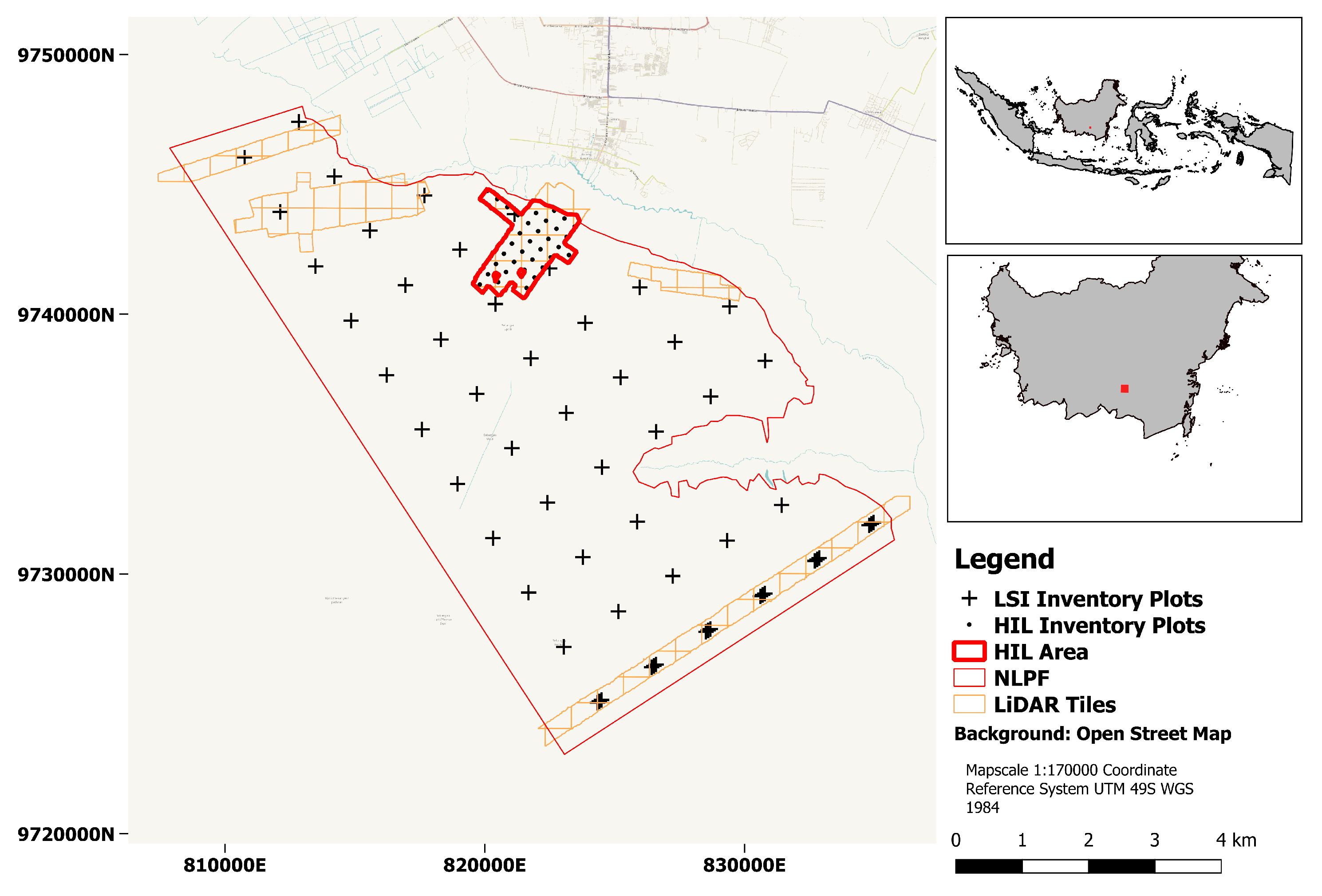
2.1. Study Area

The study area is located in Central Kalimantan, Indonesia, covering an area of 311 k m 2 in the upper catchment of the Sebangau river. The exact boundaries have been defined based on the natural borders (Sebangau River) and by the accessibility. It is part of the Natural Laboratory of Peat–Swamp Forest (NLPF) managed by the Center for International Cooperation in Sustainable Management of Tropical Peatland (CIMTROP) hosted at the University of Palangka Raya, Central Kalimantan Province, Indonesia.
The topography of the entire study area is flat and covered by an organic peat soil layer with depth varying between 1 m –9 m depending on the distance from the Sebangau river [24]. The study area is approximately 260 k m south of the Equator with a typical tropical wet climate with a mean annual temperature (2002–2010) of 26.2 C [29] and mean annual rainfall (1981–2010) of approx. 2600 m m yr −1 [30,31]. It is a habitat to a large number of ape species including Orangutan (Pongo pygmaeus wurmbii). Between 1972 and 1997, the Sebangau forest was managed as a private concession with selective logging of Ramin (Gonystylus spp.), and Meranti (Shorea sp.) species [32]. After a period of illegal logging activities between 1996 and 2004, the forest became protected as part of the Sebangau National Park by a government decree in 2004 (MoF, 2004). Altogether, forest can be described as a secondary logged-over lowland tropical peat swamp forest.

2.2. Forest Inventory Data and Allometric Biomass Model

Terrestrial field inventories were conducted by three field teams between July 2013 and June 2014. Because the ALS data did not cover the entire study area, we selected the sample plots using two independent systematic grids: (i) A Large Scale Inventory (LSI) sample grid (grid width: 2.5 k m ) covering the entire study area, and (ii) a High Intensity LiDAR (HIL) sample grid (grid width: 0.5 k m ) covering the largest patch of the ALS data. To increase the number of sample units covered by ALS data, additional samples were located along the southern border of the study area. These consists of cluster plots overlapping the center of LSI plots along with two neighboring plots at a distance of 100 m from the center of LSI plots, on each side along the main direction of the LiDAR strips (hereinafter cluster plots). In total, n = 55 plots were established in the study area: 34 HIL plots, 12 sub plots from six clusters and nine LSI plots (see Figure 1).
At each sample location, we established three nested concentric circular sub-plots with radii of 4, 8, and 16 m . Trees were selected within the three sub-plots based on their DBH values. For the smallest plots, we selected all trees with DBH ≥ 5 c m , for the medium plots those trees with DBH ≥ 17 c m and for the largest plots those with DBH ≥ 30 c m . The following attributes were observed for the selected trees: tree species, DBH, azimuth and relative distance of each tree to the plot center. The tree height was measured for 10 trees on each plot including the four trees closest to the plot center and the six trees with the largest DBH. Plot locations were measured with standard hand-held global navigation satellite system (GNSS) devices. To improve the accuracy of the localization, we averaged the position measurements for a time period of minimum 15 min .
Because AGB cannot directly be measured, a model to estimate the biomass of a single tree from a measurable variable (e.g., DBH) need to be used. The selection of such a model is a critical task in AGB assessments because it has a direct and potentially great impact on the AGB estimates [33]. However, in this work, we focused on the impact of using ALS derived auxiliary variables on the precision of AGB estimates. Thus, we were more interested in the relative difference between the two estimation approaches than in the absolute values. We further consider that the the effects of allometric model prediction uncertainty on the precision of the large area estimates are negligible relative to the effects of sampling variability. Therefore, we did not evaluate different available allometric models here and used a regional model developed for Indonesian peat swamp forests [34] with DBH and tree height as input. The DBH measurements were taken from the field inventory to calculate the biomass of each selected tree. Tree height models fitted using the trees with height measurements were used to predict the tree height of every other tree. To estimate the AGB per plot, all single tree biomasses were multiplied by the expansion factor according to the sizes of the concentric sub-plots and summed up per plot to get a plot level estimate of AGB per unit area in M g h a −1.

2.3. ALS Data and Processing

The airborne ALS data were acquired during the dry season in October 2011 using a fullwave Optech Orion M200 sensor mounted in a fixed wing aerial platform, operated at 1064 n m , a pulse repetition rate of 100 k Hz , a maximum scan angle of ± 11 , an average flying height of 800 m above the WGS84 reference ellipsoid. The data cover an area of approximately 62 k m 2 and were delivered in tiles of 1 k m with a minimum return density ranging from 0.42–7.62 returns/m 2 and a mean value of 5.2 returns/m 2 not considering overlapping flight lines. The absolute horizontal location error was reported to be < 0.07 m by the data provider.
We used FUSION software V. 3.4.2 [35] for filtering and interpolating data and generating the Digital Elevation Model (DEM), the Canopy Height Model (CHM) and the normalized height of the ALS point cloud (NH), which were necessary as input data for identifying and locating individual dominant trees and for computing ALS metrics for height and canopy cover within the limits of the field sample plots. The following processing steps were carried out:
  • Outliers were removed using the FilterData tool, considering a window size of 100 m and a maximum and minimum ellipsoidal height bound of ± 5.0 S t d . d e v .
  • The GroundFilter tool, which implements a filtering algorithm (adapted from Kraus and Pfeifer [36]) based on linear prediction [37], was used to extract ground returns from all the ALS points with a cell size of 1 m (based on available ALS data density).
  • A digital elevation model (DEM) grid with 1 m cell size was created with the GridSurfaceCreate tool which estimates the elevation of each grid cell from the lowest elevation of all points within the cell; if the cell does not contain any points, it is filled by interpolation from the neighbouring cells.
  • A canopy height model (CHM) with 1 m cell size was created using the CanopyModel tool by interpolating the first ALS pulses and subtracting the DEM elevation of each cell.
  • Finally, the ClipData tool was used to obtain the normalized heights by subtraction of the ellipsoidal height of the DEM from the ellipsoidal height of each ALS return.
In the fourth and fifth steps, we only used returns with normalized heights between 0 m –60 m , after considering the tallest trees observed in the field and to avoid errors that can occur in the filtering and interpolation processes or in the signal processing because of multiple backscatter of the laser beam.
When linking field inventory and remote sensing data, it is critical to ensure a high quality of the spatial co-registration between both datasets. From an analysis of multiple GNSS measurements on a full census plot in the same study area (data not provided here), we assume the GNSS location error to be in a magnitude of order of 10 m –16 m . For the given size of the inventory plots, this might lead to large uncertainties because the location error can be larger than the plot radius, which might lead to situations where none of the selected ALS returns is actually taken from the plot where the field observations were conducted. Depending on the spatial autocorrelation structure of the forest, this will lead to an increase in uncertainty. In order to improve the co-registration, we developed a semi-automatic co-registration protocol. The co-registration is based on the identification of dominant trees from the inventory plots and in the ALS point cloud (details are provided in [38]).
The prediction of AGB based on the ALS data followed the standard area-based approach first described by Næsset [39] that uses ALS-derived metrics calculated from the NH as explanatories. To obtain these metrics, we performed the following processes using the FUSION software: (i) the normalized ALS point cloud was clipped using the PolyClipData tool within the limits of each field plot (which were previously stored as polygons in shapefiles), and we created an independent file for each plot of 16 m radius and (ii) the CloudMetrics tool was used to estimate height and canopy cover metrics of these 55 clipped and normalized point clouds. The ALS metrics were computed using all normalized returns. The minimum height threshold (MHT), which is commonly specified as the lower boundary for calculating height metrics (central tendency, dispersion, shape and percentile statistics), was established at 2.5 m to exclude grasses and shrubs. The height break threshold (HBT), which is the limit for separating the point cloud data into two sets to separate canopy returns from the understory returns, in order to estimate canopy cover metrics, was established at 6.5 m (based on field observations). In total, 39 metrics widely used to predict AGB [40] were extracted from NH and used as predictors in the statistical analysis. The ALS metrics and the corresponding descriptions for height distribution and canopy closure are summarized in Table 1.
Finally, because we were also interested in the construction of a AGB map for the HIL area, we generated 39 rasters of 30 m cell size (chosen to match the scale of prediction to the size of the field plot observations, i.e., 804 m 2 ) for each of the statistics described in Table 1 using the GridMetrics tool.

2.4. Building the Biomass-Link Model

As a biomass-link model to predict plot level AGB estimates from the ALS metrics, we used a nonlinear logistic regression model as described by McRoberts et al. [41]:
y i = f ( X i ; β ) = β J + 2 1 + exp ( β J + 1 + j = 1 J β j X i j ) + ϵ i ,
where i is the plot index, j indexes the ALS predictor metrics so that X i j is j’th ALS metrics observed on plot i. β is the vector of regression parameters to be estimated and ϵ is the residual error term. This model type was selected because it fits the properties of the target variable AGB. All predictions are non-negative and in between a lower ( y ^ = 0 ) and upper asymptotic bound ( y ^ = β ^ J + 2 ), which is estimated from the inventory data [41].
The usage of the model-assisted difference estimators requires a probability sample [42] when estimating bias and variance. However, to build the model itself, such an assumption is not required and external data can be utilized (see e.g., [43]). In the study at hand, we follow this approach and use all n = 55 observations from the different sampling grids to fit the regression model. However, inference on AGB estimates are restricted to the HIL area where the points were collected following a systematic sample design.
The limited number of field plots ( n = 55 ), the large number of ALS metrics as potential predictors (39) and the fact that many of the ALS metrics carry redundant information are causing problems when fitting parametric models. To reduce the chance of overfitting and to keep the model simple, a feature selection was done. However, feature selection for parametric nonlinear regression models is subject to active research and most of the suggested methods are complex and lag generality. Therefore, we decided to follow a simplified approach based on linear models. We are fully aware that a linear approach might not select the best set of predictor variables for nonlinear models in all cases. However, because of the lack of a general feature selection method for parametric nonlinear regression models and the fact that this approach has been proven before [44], we consider this option as a viable and valid one. For the feature selection, we tested all possible combinations of maximal five predictors in an exhaustive feature selection using the leaps package [45] of the statistical software R [46]. We selected the model with the lowest residual standard error (RSE) and removed all terms with a variance inflation factor (VIF) > 10 . We then fitted the nonlinear model (see Equation (1)) with the selected features using unweighted least square estimates as implemented in the nls function of R [46]. Finally, we removed all non-significant (p-value > 0.005 ) terms from the nonlinear model.

2.5. AGB Estimation

For the estimation of the AGB mean μ ^ and its error variance v a r ^ , we used two approaches: (i) the field-based approach which uses the field inventory data only, and (ii) the ALS-assisted approach which uses the field data and the selected ALS metrics as information sources. For the field-based approach, we used the estimators described in Särndal et al. [20] and estimate the mean μ ^ F I E L D AGB in M g h a −1 and its error variance v a r ^ F I E L D for n plots with the estimated variance σ ^ 2 as follows:
μ ^ F I E L D = 1 n i = 1 n y i ,
v a r ^ ( μ ^ F I E L D ) = σ ^ 2 n .
For the ALS-assisted approach, we used the model-assisted framework, which was presented in Särndal et al. [20] and which has been successfully utilized for ALS based forest biomass and volume assessments before [15,21,41]. We estimate the ALS-assisted mean μ ^ A L S AGB in M g h a −1 and its error variance v a r ^ A L S for n plots with the model residuals ϵ i = y ^ i y i for all N sampling units (here pixel) as follows:
μ ^ A L S = 1 N k = 1 N y k ^ 1 n i = 1 n ( y i ^ y i ) ,
v a r ^ ( μ ^ A L S ) = 1 n ( n 1 ) i = 1 n ( ϵ i ϵ ¯ ) 2 .

3. Results

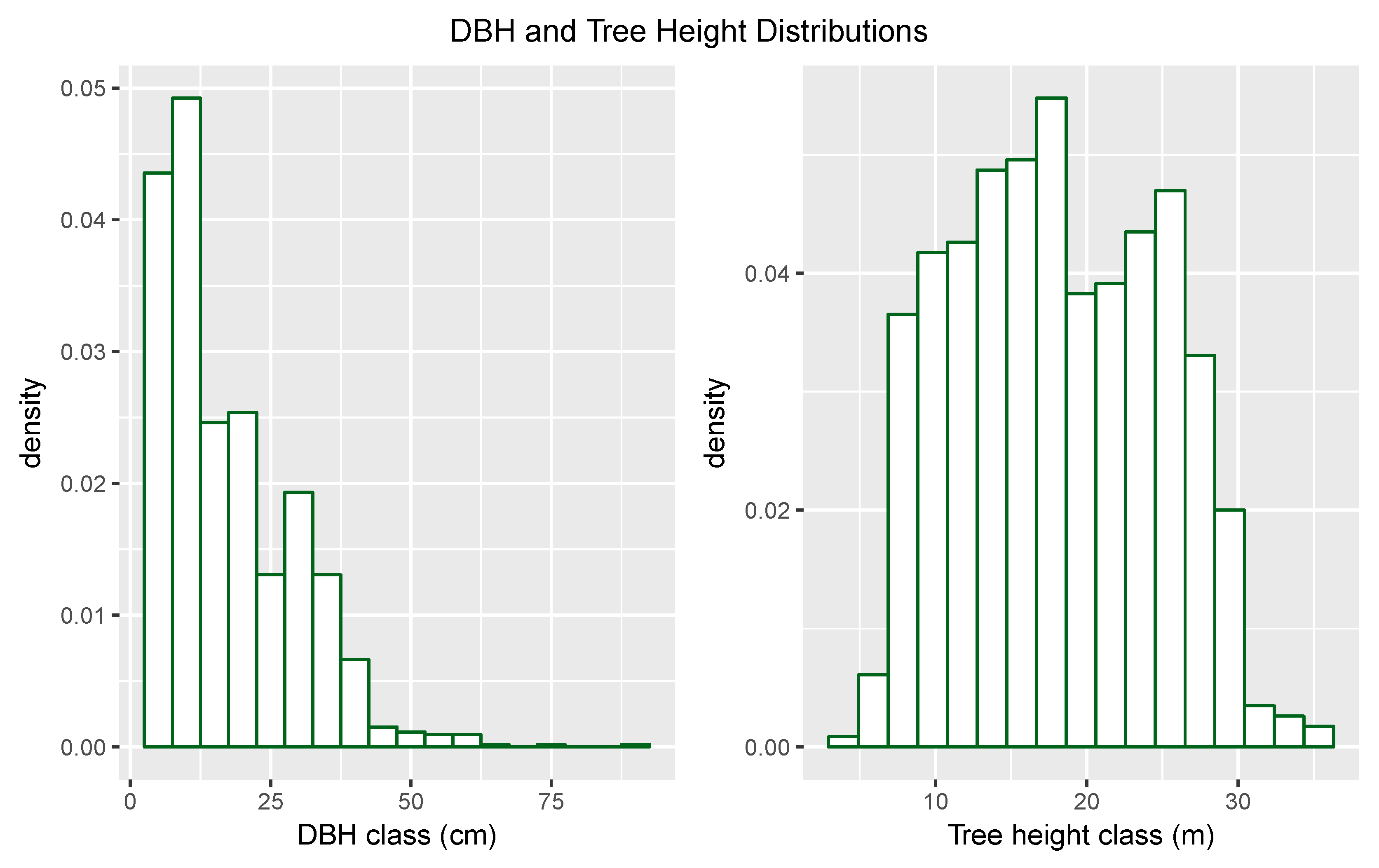
3.1. Forest Inventory Results

The analysis of the forest inventory data showed that the part of the Sebangau forest covered by the HIL plots is very homogeneous with relatively small mean DBH values and a large number of stems (see Table 2). The DBH distribution shows the typical self-thinning curve of a secondary forest with a large number of trees with small DBH and an exponentially decreasing number of trees for higher DBH classes (see Figure 2). Because of the logging history, very large trees with DBH ≥ 60 c m are rare. The tree heights show an irregular distribution without much differentiation and a relatively low mean tree height of 17.5 m . The distribution indicates that there is no single dominant tree layer but a very complex vertical forest structure with trees in many different height classes as shown in the photo in Figure 3. Thus, the DBH and tree height distributions reflect the management history characterizing the forest as logged-over secondary forest, where larger trees have been taken out and natural regeneration is filling the gaps. The forest hosts a large number of tree species (129 species observed on all plots). However, the allometric model that was used for estimating the single tree AGB is a mixed species model [34]. Therefore, the large number of tree species does not contribute to the variation of AGB on the plot level in our analysis.
Among the presented forest structure variables, the stem density has the highest coefficient of variation, whereas the variation of mean tree heights between the plots is small. From the field work and the analysis of the tree height distribution, the vertical forest structure can be described as complex. However, the small CV of the mean tree heights indicates that the complex vertical structure is homogeneously covering the study area. The differences in the plot level AGB estimates are mainly attributed to variations in the stem density as shown in Table 2. As shown in Figure 4 more than 75% of the total AGB can be found in trees with DBH ≤ 30 c m .

3.2. Biomass-Link Model

We started building the biomass-link model by selecting the ALS predictor variables. The exhaustive search for the best linear AGB prediction model showed only little improvement for models with more than five independent variables. The final model with the smallest RSE included the 5% percentile ( h 05 ) and the median of the absolute deviations from the overall median ( h M A D m e d i a n ) as significant predictors, which resulted in an RMSE of 47.43 M g h a −1. To evaluate the model quality, we present diagnostic plots in Figure 5. The slope of the observed versus predicted was estimated to be 1.01. However, the subplot of the observed means versus predicted means indicates a poor quality of the fit because the slope of the observed against predicted line is significantly different from 1 and the intercept is different from 0. As a consequence, the predictions from the nonlinear logistic biomass-link model will overestimate AGB values up to a threshold of approx. 225 M g h a −1 and underestimate the AGB for larger values.
We used the biomass-link model to create a map of AGB predictions for the HIL area as shown in Figure 6. The visual check of the spatial distribution of the AGB seems plausible. For example, the tracks that were formally cut to extract saw logs on small train tracks are clearly visible. However, from the map, no spatial trends in AGB density can be observed nor any other particular spatial pattern. Thus, the AGB map confirms the results from the forest inventory showing a homogeneous forest structure for the HIL area.

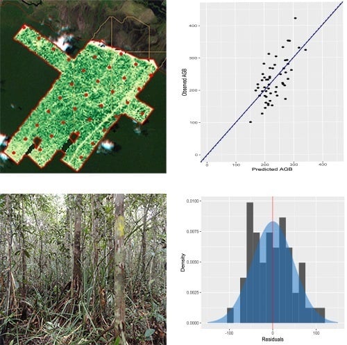
3.3. Comparison of the AGB Estimates

The evaluation of the forest inventory data confirmed the homogeneous forest structure. With only 34 plots in the HIL area, the mean AGB stock was estimated with a quite high precision as expressed by the small relative standard error of 4.63 % of the mean. Given this fact plus the low model quality of the biomass-link model, only little improvements in the precision of the ALS-assisted estimates can be expected. In Table 3, both estimates are compared. The mean AGB estimates of both approaches are very similar. The standard error is 0.6 M g h a −1 smaller for the ALS-assisted approach, which indicates a slightly higher precision when using ALS and forest inventory data.

4. Discussion

The potential of remote sensing technologies for monitoring forest biomass stocks in the tropics has been evaluated by many [8,47,48,49]. However, most of the works are focusing on the biomass-link model and evaluate their quality from the residuals between observations and model predictions. Even though the quality of the biomass-link model is an important determinant of the precision of the model predictions, it is by no means a good predictor for the precision of the AGB estimates when applied for larger forest areas because models need to be evaluated in context of their application [50]. In cases where statistical point and interval estimates are to be given, further analyses beyond the evaluation of the biomass-link model are required, or, in other words: if statistical inference should be made instead of “pretty pictures”, statistical inference frameworks need to be applied [51].
The analysis of the inventory data considering only the field-based information resulted in an estimated mean biomass of 241.38 M g h a −1, which corresponds well to other biomass assessments conducted in the same study area. Kronseder et al. [28] reported a mean AGB of 258.5 M g h a −1 and Campbell [32] reported a higher mean AGB value of 297.8 M g h a −1 from five plots in the same study area. Englhart et al. [52] reported a mean AGB of 203.0 M g h a −1 for a peat–swamp forest area that partly covers the study area. Thus, the field-based point estimates can be considered plausible. Because the listed studies were not design-based nor were the standard errors given, we cannot compare our interval estimates e.g., the standard error of 11.17 M g h a −1 to other studies conducted in this region.
The biomass-link model used in this study has an RSE of 47.43 M g h a −1, which is in the range of other studies that use ALS data to predict biomass in tropical forests. Zolkos et al. [53] conducted a meta-analysis of such studies and reported a median RSE for tropical forest types of 40 M g h a −1. Even though, the RSE was within the range of other studies, the predictive power of the model is limited since the relationship between AGB and ALS metrics was weak. This is indicated e.g., by the Pearson correlation coefficient of 0.65 for the predicted versus observed AGB values. A similar finding is reported by Palace et al. [54] who used discrete return ALS metrics to describe the forest structure, including biomass, of a complex tropical forest in La Selva, Costa Rica. They found no significant relationship between ALS height metrics and AGB and concluded that alternative metrics need to be found for predicting AGB at local scales [54]. In addition, Vaglio Laurin et al. [49] reported that the upper height percentiles have only a limited predictive power for AGB in a tropical forest in Africa. They attributed this effect to the multi-layered forest structure where most of the biomass is found in the sub-canopy trees. In Sebangau, forest variation is caused mainly by differences in the tree densities and not so much to variations in the canopy heights. Other studies showed stronger relationships between ALS height metrics and AGB for tropical forests. Ioki et al. [48] created univariate linear biomass-link models to predict AGB in tropical forests of northern Kalimantan using ALS data that had coefficients of variation > 0.7 .
The ALS data used in the study is comparable to other studies that predict forest AGB. The ALS processing followed a standard area-based approach and was conducted with standard algorithms. Thus, we assume that the data processing had only a minor effect on the quality of the AGB and ALS metrics relation. Among the reasons why the relationships are weaker in our study may be the following: (i) the forest structure in the study area is characterized by a high tree density (>2000 trees per ha), a small mean DBH and little variation in DBH and height. In general, the forest can be described as a closed canopy forest with very little variation of the AGB estimates at plot scale. As many of the ALS metrics describe the height distribution of the canopy, their explanatory power is obviously limited for these forest conditions, (ii) in a pan-tropical study, Slik et al. [55] showed that the density of large trees (DBH > 70 c m ) has a large influence on the variations of AGB. The largest DBH found in the HIL study area was 63.3 c m and only 1.5% were larger then 50 c m so that the general absence of scattered large trees is another potential explanation for the little variation of the AGB values in the HIL area, and (iii) the plot design can have a great influence on the relationship between any forest variable and remote sensing observation because it determines the scale at which the relation is modeled. Mascaro et al. [56] analyzed the model qualities of ALS biomass-link models for different resolutions and formulated a scaling rule for the RMSE. Mauya et al. [57] showed that the precision of ALS-assisted AGB estimates is also affected by the field plot size. They concluded that increasing the field plot size reduces boundary effects, which leads to better prediction models. However, larger plot sizes are not efficient when it comes to field sampling because implementing larger plots in the field is difficult and time consuming and thus reduces the number of plots that can be implemented with a given budget, and (iv) there is a time gap of up to three years between the ALS acquisition and the field observations, which could reduce the correlations in cases of changes in the forest structure. However, because this is a protected forest area, we assume that there are no logging activities in the study area. This is also confirmed by other research groups who maintain a field station and carry out regular monitoring in that area. Thus, we consider structural changes in the period 2011–2014 to be very minor in the studied area.
Given the limited correlation between the ALS metrics and the observed AGB values in our study area, the gain in precision when estimating AGB by combining forest inventory and remote sensing data was small. Thus, for the given situation, the investment in the ALS data acquisition could not be justified by the gain in efficiency. To achieve a confidence interval similar to the ALS-assisted using the field-based approach, a sample size of n = 37 would be needed. Thus, increasing the sample size by three more plots would have resulted in a similar confidence interval but with much lower costs when compared to conducting an ALS data acquisition and analysis. In addition, the add-on product of a wall-to-wall map was not very informative in our study because the spatial distribution of AGB is homogeneous and thus only little additional information is being gained from the map. However, for a designer of a forest monitoring program, it is currently not easy to make a decision beforehand whether it is worth investing in ALS data or not. Therefore, techniques that allow a pre-survey determination of the expected gain in precision are demanded. One such approach could be based on the analysis of the spatial auto-correlation patterns in the freely available satellite images as provided by Landsat 8 or Sentinel 2. If such a pilot survey reveals a long-range spatial correlation of the plots with little variability, a gain in precision is unlikely. Thus, methods that allow (i) predicting the homogeneity in advance, and (ii) finding a threshold of variation where an economically meaningful inclusion is required.

5. Conclusions

Based on the findings from this study, we draw the following conclusions:
  • The usage of expensive ALS data in forest monitoring programs cannot always be justified by an actual gain in precision,
  • Model-assisted estimators provide a good framework to examine the gain in precision and to evaluate the advantage of using different remote sensing products,
  • As different studies report different ’gain’ in precision from using ALS data, further research is required to inform forest monitoring systems on the expected gain of collecting additional remote sensing products before the monitoring is implemented.

Author Contributions

All authors actively contributed to the manuscript through their review, editing and comments. P.M. took the lead and was involved in the fieldwork and project design and all steps of the data analysis. E.G.-F. contributed to the LiDAR data processing in FUSION, E.S.P. was involved in the fieldwork and implemented the positional correction procedure. D.S. was involved in the organization of the fieldwork and contributed to the analysis of the data. C.P.-C. contributed to the modeling of AGB and tree height and in designing the study. C.K. was involved in all stages of the project and contributed to the discussion and inventory design.

Funding

We are grateful for the financial support of the German Research Foundation DFG who funded the project (KL-895/17) and the Galician Government and European Social Fund (Official Journal of Galicia—DOG n 52, 17/03/2014 p. 11343, exp: POS-A/2013/049) for funding the postdoctoral research stays of Eduardo González-Ferreiro in Göttingen.

Acknowledgments

The authors would like to thank the late Suwido Limin and his team at the Center for International Cooperation in Sustainable Management of Tropical Peatland (CIMTROP) who supported the fieldwork. We also like to acknowledge Florian Siegert for his support in setting up this project. Additionally, the authors would like to thank Ron E. McRoberts and two anonymous reviewers for their expertise and perspectives that helped improve the quality of the final manuscript.

Conflicts of Interest

The authors declare no conflict of interest.

References

  1. Pan, Y.; Birdsey, R.A.; Fang, J.; Houghton, R.; Kauppi, P.E.; Kurz, W.A.; Phillips, O.L.; Shvidenko, A.; Lewis, S.L.; Canadell, J.G.; et al. A large and persistent carbon sink in the world’s forests. Science 2011, 333, 988–993. [Google Scholar] [CrossRef] [PubMed]
  2. Drake, J.B.; Knox, R.G.; Dubayah, R.O.; Clark, D.B.; Condit, R.; Blair, J.B.; Hofton, M. Above-ground biomass estimation in closed canopy Neotropical forests using lidar remote sensing: Factors affecting the generality of relationships. Glob. Ecol. Biogeogr. 2003, 12, 147–159. [Google Scholar] [CrossRef]
  3. Barrett, F.; Mcroberts, R.E.; Tomppo, E.; Cienciala, E.; Waser, L.T. A questionnaire-based review of the operational use of remotely sensed data by national forest inventories. Remote Sens. Environ. 2016, 174, 279–289. [Google Scholar] [CrossRef]
  4. Sader, S.A.; Waide, R.B.; Lawrence, W.T.; Joyce, A.T. Tropical forest biomass and successional age class relationships to a vegetation index derived from landsat TM data. Remote Sens. Environ. 1989, 28, 143–198. [Google Scholar] [CrossRef]
  5. Eckert, S. Improved forest biomass and carbon estimations using texture measures from worldView-2 satellite data. Remote Sens. 2012, 4, 810–829. [Google Scholar] [CrossRef]
  6. Nichol, J.E.; Sarker, M.L.R. Improved Biomass Estimation Using the Texture Parameters of Two High-Resolution Optical Sensors. IEEE Trans. Geosci. Remote Sens. 2011, 49, 930–948. [Google Scholar] [CrossRef] [Green Version]
  7. Dobson, M.; Ulaby, F.; LeToan, T.; Beaudoin, A.; Kasischke, E.; Christensen, N. Dependence of radar backscatter on coniferous forest biomass. IEEE Trans. Geosci. Remote Sens. 1992, 30, 412–415. [Google Scholar] [CrossRef]
  8. Asner, G.P.; Mascaro, J.; Muller-Landau, H.C.; Vieilledent, G.; Vaudry, R.; Rasamoelina, M.; Hall, J.S.; van Breugel, M. A universal airborne LiDAR approach for tropical forest carbon mapping. Oecologia 2012, 168, 1147–1160. [Google Scholar] [CrossRef] [PubMed]
  9. Næsset, E. Estimating timber volume of forest stands using airborne laser scanner data. Remote Sens. Environ. 1997, 61, 246–253. [Google Scholar] [CrossRef]
  10. Hyyppä, J.; Hyyppä, H.; Leckie, D.; Gougeon, F.; Yu, X.; Maltamo, M. Review of methods of small—Footprint airborne laser scanning for extracting forest inventory data in boreal forests. Int. J. Remote Sens. 2008, 29, 1339–1366. [Google Scholar] [CrossRef]
  11. Lefsky, M.A.; Harding, D.; Cohen, W.; Parker, G.; Shugart, H. Surface Lidar Remote Sensing of Basal Area and Biomass in Deciduous Forests of Eastern Maryland, USA. Remote Sens. Environ. 1999, 67, 83–98. [Google Scholar] [CrossRef] [Green Version]
  12. Nelson, R.; Short, A.; Valenti, M. Measuring biomass and carbon in delaware using an airborne profiling LIDAR. Scand. J. For. Res. 2004, 19, 500–511. [Google Scholar] [CrossRef]
  13. Koch, B. Status and future of laser scanning, synthetic aperture radar and hyperspectral remote sensing data for forest biomass assessment. ISPRS J. Photogramm. Remote Sens. 2010, 65, 581–590. [Google Scholar] [CrossRef]
  14. Lu, D. The potential and challenge of remote sensing—Based biomass estimation. Int. J. Remote Sens. 2006, 27, 1297–1328. [Google Scholar] [CrossRef]
  15. Gregoire, T.G.; Ståhl, G.; Næsset, E.; Gobakken, T.; Nelson, R.; Holm, S. Model-assisted estimation of biomass in a LiDAR sample survey in Hedmark County, NorwayThis article is one of a selection of papers from Extending Forest Inventory and Monitoring over Space and Time. Can. J. For. Res. 2011, 41, 83–95. [Google Scholar] [CrossRef]
  16. Ståhl, G.; Holm, S.; Gregoire, T.G.; Gobakken, T.; Næsset, E.; Nelson, R. Model-based inference for biomass estimation in a LiDAR sample survey in Hedmark County, Norway. Can. J. of For. Res. 2011, 41, 96–107. [Google Scholar] [CrossRef]
  17. Næsset, E.; Gobakken, T.; Bollandsås, O.M.; Gregoire, T.G.; Nelson, R.; Ståhl, G. Comparison of precision of biomass estimates in regional field sample surveys and airborne LiDAR-assisted surveys in Hedmark County, Norway. Remote Sens. Environ. 2013, 130, 108–120. [Google Scholar] [CrossRef]
  18. McRoberts, R.E. A model-based approach to estimating forest area. Remote Sens. Environ. 2006, 103, 56–66. [Google Scholar] [CrossRef]
  19. Opsomer, J.D.; Breidt, F.J.; Moisen, G.G.; Kauermann, G. Model-assisted estimation of forest resources with generalized additive models. J. Am. Stat. Assoc. 2007, 102, 400–409. [Google Scholar] [CrossRef]
  20. Särndal, C.E.; Swensson, B.; Wretman, J. Model Assisted Survey Sampling; Springer: Berlin, Germany, 1992. [Google Scholar]
  21. Næsset, E.; Gobakken, T.; Solberg, S.; Gregoire, T.G.; Nelson, R.; Ståhl, G.; Weydahl, D. Model-assisted regional forest biomass estimation using LiDAR and InSAR as auxiliary data: A case study from a boreal forest area. Remote Sens. Environ. 2011, 115, 3599–3614. [Google Scholar] [CrossRef]
  22. Næsset, E.; Ørka, H.O.; Solberg, S.; Bollandsås, O.M.; Hansen, E.H.; Mauya, E.; Zahabu, E.; Malimbwi, R.; Chamuya, N.; Olsson, H.; et al. Mapping and estimating forest area and aboveground biomass in miombo woodlands in Tanzania using data from airborne laser scanning, TanDEM-X, RapidEye, and global forest maps: A comparison of estimated precision. Remote Sens. Environ. 2016, 175, 282–300. [Google Scholar] [CrossRef]
  23. D’Oliveira, M.V.N.; Reutebuch, S.E.; McGaughey, R.J.; Andersen, H.E. Estimating forest biomass and identifying low-intensity logging areas using airborne scanning lidar in Antimary State Forest, Acre State, Western Brazilian Amazon. Remote Sens. Environ. 2012, 124, 479–491. [Google Scholar] [CrossRef]
  24. Page, S.E.; Rieley, J.O.; Shotyk, W.; Weiss, D. Interdependence of peat and vegetation in a tropical peat swamp forest. Philos. Trans. R. Soc. Lond. Ser. B Biol. Sci. 1999, 354, 1885–1897. [Google Scholar] [CrossRef] [PubMed]
  25. Ballhorn, U.; Jubanski, J.; Kronseder, K. Airborne LiDAR measurements to estimate tropical peat swamp forest aboveground Biomass. In Proceedings of the International Geoscience and Remote Sensing Symposium, Munich, Germany, 22–27 July 2012; pp. 1660–1663. [Google Scholar]
  26. Ballhorn, U.; Jubanski, J.; Siegert, F. ICESat/GLAS data as a measurement tool for peatland topography and peat swamp forest biomass in Kalimantan, Indonesia. Remote Sens. 2011, 3, 1957–1982. [Google Scholar] [CrossRef] [Green Version]
  27. Jubanski, J.; Ballhorn, U.; Kronseder, K.; Franke, J.; Siegert, F. Detection of large above-ground biomass variability in lowland forest ecosystems by airborne LiDAR. Biogeosciences 2013, 10, 3917–3930. [Google Scholar] [CrossRef] [Green Version]
  28. Kronseder, K.; Ballhorn, U.; Böhm, V.; Siegert, F. aboveground biomass estimation across forest types at different degradation levels in Central Kalimantan using LiDAR data. Int. J. Appl. Earth Obs. Geoinform. 2012, 18, 37–48. [Google Scholar] [CrossRef]
  29. Hirano, T.; Kusin, K.; Limin, S.; Osaki, M. Carbon dioxide emissions through oxidative peat decomposition on a burnt tropical peatland. Glob. Chang. Biol. 2014, 20, 555–565. [Google Scholar] [CrossRef] [PubMed]
  30. BMKG. Prakiraan Musim Hujan 2014/2015 di Indonesia; Badan Meteorologi Klimatology dan Geofisika: Jakarta, Indonesia, 2014. [Google Scholar]
  31. Harrison, M.E. Orang-Utan Feeding Behaviour in Sabangau, Central Kalimatan. Ph.D. Thesis, University of Cambridge, Cambridge, UK, 2009. [Google Scholar]
  32. Campbell, L.A.D. Disturbance Effects on Carbon Content and Tree Species Traits in Tropical Peat Swamp Forest in Central Kalimantan, Indonesian Borneo. Bachelor’s Thesis, Dalhousie University, Halifax, NS, Canada, 2013. [Google Scholar]
  33. Pérez-Cruzado, C.; Fehrmann, L.; Magdon, P.; Cañellas, I.; Sixto, H.; Kleinn, C. On the site-level suitability of biomass models. Environ. Model. Softw. 2015, 73, 14–26. [Google Scholar] [CrossRef]
  34. Manuri, S.; Brack, C.; Nugroho, N.P.; Hergoualc’h, K.; Novita, N.; Dotzauer, H.; Verchot, L.; Putra, C.A.S.; Widyasari, E. Tree biomass equations for tropical peat swamp forest ecosystems in Indonesia. For. Ecol. Manag. 2014, 334, 241–253. [Google Scholar] [CrossRef]
  35. McGaughey, J.R. FUSION/LDV: Software for LIDAR Data Analysis and Visualization; United States Department of Agriculture, Forest Service, Pacific Northwest Research Station, University of Washington: Seattle, WA, USA, 2014. [Google Scholar]
  36. Kraus, K.; Pfeifer, N. Determination of terrain models in wooded areas with airborne laser scanner data. ISPRS J. Photogramm. Remote Sens. 1998, 53, 193–203. [Google Scholar] [CrossRef]
  37. Kraus, K.; Mikhail, E. Linear least squares interpolation. Photogramm. Eng. 1972, 635, 1016–1029. [Google Scholar]
  38. Magdon, P.; Purnama, E.; Sarodja, D.; Perez-Cruzado, C. Estimating aboveground biomass using small footprint LiDAR data in tropical peat–swamp forests. -A case study from Central Kalimantan-. In The Ecological and Economic Challanges of Managing Forested Landscapes in a Global Context; Cuvillier Verlag: Göttingen, Germany, 2014. [Google Scholar]
  39. Næsset, E. Predicting forest stand characteristics with airborne scanning laser using a practical two-stage procedure and field data. Remote Sens. Environ. 2002, 80, 88–99. [Google Scholar] [CrossRef]
  40. Gonzalez-Ferreiro, E.; Miranda, D.; Barreiro-Fernandez, L.; Bujan, S.; Garcia-Gutierrez, J.; Dieguez-Aranda, U. Modelling stand biomass fractions in Galician eucalyptus globulus plantations by use of different LiDAR pulse densities. For. Syst. 2013, 22, 510–525. [Google Scholar] [CrossRef]
  41. McRoberts, R.E.; Næsset, E.; Gobakken, T. Inference for lidar-assisted estimation of forest growing stock volume. Remote Sens. Environ. 2013, 128, 268–275. [Google Scholar] [CrossRef]
  42. McRoberts, R.E.; Walters, B.F. Statistical inference for remote sensing-based estimates of net deforestation. Remote Sens. Environ. 2012, 124, 394–401. [Google Scholar] [CrossRef]
  43. Kangas, A.; Myllymäki, M.; Gobakken, T.; Næsset, E. Model-assisted forest inventory with parametric, semi-parametric and non-parametric models. Can. J. For. Res. 2016, 868. [Google Scholar] [CrossRef]
  44. Fuchs, H.; Magdon, P.; Kleinn, C.; Flessa, H. Estimating aboveground carbon in a catchment of the Siberian forest tundra: Combining satellite imagery and field inventory. Remote Sens. Environ. 2009, 113, 518–531. [Google Scholar] [CrossRef]
  45. Lumley, T. Leaps: Regression Subset Selection. 2009. R Package Version 2.9. Available online: http://CRAN.R-project.org/package=leaps (accessed on 3 August 2018 ).
  46. R Core Team. R: A Language and Environment for Statistical Computing; R Foundation for Statistical Computing: Vienna, Austria, 2016. [Google Scholar]
  47. Clark, M.L.; Roberts, D.A.; Ewel, J.J.; Clark, D.B. Estimation of tropical rain forest aboveground biomass with small-footprint lidar and hyperspectral sensors. Remote Sens. Environ. 2011, 115, 2931–2942. [Google Scholar] [CrossRef]
  48. Ioki, K.; Tsuyuki, S.; Hirata, Y.; Phua, M.H.; Wong, W.V.C.; Ling, Z.Y.; Saito, H.; Takao, G. Estimating above-ground biomass of tropical rainforest of different degradation levels in Northern Borneo using airborne LiDAR. For. Ecol. Manag. 2014, 328, 335–341. [Google Scholar] [CrossRef]
  49. Vaglio Laurin, G.; Chen, Q.; Lindsell, J.A.; Coomes, D.A.; Frate, F.D.; Guerriero, L.; Pirotti, F.; Valentini, R. Aboveground biomass estimation in an African tropical forest with lidar and hyperspectral data. ISPRS J. Photogramm. Remote Sens. 2014, 89, 49–58. [Google Scholar] [CrossRef]
  50. McRoberts, R.E.; Chen, Q.; Domke, G.M.; Ståhl, G.; Saarela, S.; Westfall, J.A. Hybrid estimators for mean aboveground carbon per unit area. For. Ecol. Manag. 2016, 378, 44–56. [Google Scholar] [CrossRef]
  51. McRoberts, R.E. Satellite image-based maps: Scientific inference or pretty pictures? Remote Sens. Environ. 2011, 115, 715–724. [Google Scholar] [CrossRef]
  52. Englhart, S.; Jubanski, J.; Siegert, F. Quantifying Dynamics in Tropical Peat Swamp Forest Biomass with Multi-Temporal LiDAR Datasets. Remote Sens. 2013, 5, 2368–2388. [Google Scholar] [CrossRef] [Green Version]
  53. Zolkos, S.G.; Goetz, S.J.; Dubayah, R. A meta-analysis of terrestrial aboveground biomass estimation using lidar remote sensing. Remote Sens. Environ. 2013, 128, 289–298. [Google Scholar] [CrossRef]
  54. Palace, M.W.; Sullivan, F.B.; Ducey, M.J.; Treuhaft, R.N.; Herrick, C.; Shimbo, J.Z.; Mota-E-Silva, J. Estimating forest structure in a tropical forest using field measurements, a synthetic model and discrete return lidar data. Remote Sens. Environ. 2015, 161, 1–11. [Google Scholar] [CrossRef]
  55. Slik, J.W.F.; Paoli, G.; Mcguire, K.; Amaral, I.; Barroso, J.; Bastian, M.; Blanc, L.; Bongers, F.; Boundja, P.; Clark, C.; et al. Large trees drive forest aboveground biomass variation in moist lowland forests across the tropics. Glob. Ecol. Biogeogr. 2013, 22, 1261–1271. [Google Scholar] [CrossRef]
  56. Mascaro, J.; Detto, M.; Asner, G.P.; Muller-Landau, H.C. Evaluating uncertainty in mapping forest carbon with airborne LiDAR. Remote Sens. Environ. 2011, 115, 3770–3774. [Google Scholar] [CrossRef] [Green Version]
  57. Mauya, E.W.; Hansen, E.H.; Gobakken, T.; Bollandsås, O.M.; Malimbwi, R.E.; Næsset, E. Effects of field plot size on prediction accuracy of aboveground biomass in airborne laser scanning-assisted inventories in tropical rain forests of Tanzania. Carbon Balance Manag. 2015, 10, 1–14. [Google Scholar] [CrossRef] [PubMed] [Green Version]
Figure 1. Location of the study area, the ALS tiles and the two systematic sampling grids: (i) High Intensity LiDAR (HIL) and (ii) Large Scale Inventory (LSI). All plots that are covered by LiDAR tiles were used as ALS training plots.
Remotesensing 10 01344 g001
Figure 2. Diameter and tree height distributions as observed on the HIL plots
Remotesensing 10 01344 g002
Figure 3. Photo of the complex vertical forest structure of the study area in Sebangau forest, Kalimantan.
Remotesensing 10 01344 g003
Figure 4. Distribution of the total biomass over 5 c m diameter classes for the HIL plots.
Remotesensing 10 01344 g004
Figure 5. Plots for analyzing the biomass-link model with the AGB observations versus nonlinear logistic model predictions (top left), model residuals versus observed AGB values (top right), histogram of the residuals including a normal distribution curve (blue) with the same mean and standard deviation (lower left), and mean value of predicted AGB versus mean value of observed AGB values. All AGB values are in M g / h a
Remotesensing 10 01344 g005
Figure 6. Map of ALS-assisted AGB predictions for the HIL area with 30 m spatial resolution.
Remotesensing 10 01344 g006
Table 1. ALS point cloud metrics calculated from the height distribution of the normalized returns for each inventory plot.
Variables Related to Height
Distribution (m)Description
h m a x maximum
h m e a n mean
h m o d e mode
h S D standard deviation
h V variance
h C V coefficient of variation
h I Q interquartile range
h s k w skewness
h k u r t kurtosis
h A A D average absolute deviation
h M A D m e d i a n median of the absolute deviations from the overall median
h M A D m o d e median of the absolute deviations from the overall mode
h L 1 , L 2 , , L 4 L-moments
h L s k w L-moment skewness
h L k u r L-moment kurtosis
h L C V L-moment coefficient of variation
h 01 , 05 , 10 , 20 , 25 , 30 , 70 , 75 , 80 , 90 , 95 , 99 percentiles
h q m e a n Quadratic mean
h c m e a n Cubic mean
Variables Related to
Canopy ClosureDescription
P F R A h m e a n ratio of the number of the first laser returns above h m e a n to the number of first laser returns for each plot
P F R A h m o d e ratio of the number of the first laser returns above h m o d e to the number of first returns for each plot
P A R A h m e a n ratio of the number of the all laser returns above h m e a n to the number of all laser returns for each plot
P A R A h m o d e ratio of the number of the all laser returns above h m o d e to the number of all laser returns for each plot
P F R A 6 ratio of the number of the first laser returns above 6 meter height to the total number of first laser returns for each plot
P A R A 6 ratio of the number of the all laser returns above 6 m height to the total number of first laser returns for each plot
C R R Canopy relief ratio ((mean−min)/(max−min))
Table 2. Descriptive statistics of the plot level inventory results from the HIL plots ( n = 34 ) including the Coefficient of Variation (CV).
Target VariableMeanMinimumMaximumCV %
Mean DBH ( c m )18.711.12520.2
Mean Height ( m )17.410.623.216.5
Basal Area ( m 2 h a −1)30.217.542.222.9
Stems per ha21661069482433.3
AGB ( M g h a −1)241.4100.9352.827.0
Table 3. Estimates of mean aboveground Biomass (AGB) per unit area ( M g h a −1).
EstimatornN μ ^ v a ^ r ( μ ^ ) SE ( μ ^ ) SE % ( μ ^ )
field-based34241.38124.8111.174.63%
ALS-assisted349480245.08111.6610.574.30%

