Estimates of Daily PM2.5 Exposure in Beijing Using Spatio-Temporal Kriging Model


1
College of Geographical Science, Fujian Normal University, Fuzhou 350007, China
2
State Key Laboratory of Resources and Environmental Information System, Institute of Geographical Sciences and Natural Resources Research, Chinese Academy of Sciences, Beijing 100101, China
3
College of Tourism, Fujian Normal University, Fuzhou 350117, China
*
Authors to whom correspondence should be addressed.
Sustainability 2018, 10(8), 2772; https://doi.org/10.3390/su10082772
Submission received: 12 July 2018
/
Revised: 2 August 2018
/
Accepted: 3 August 2018
/
Published: 6 August 2018
Abstract
:Excessive exposure to ambient (outdoor) air pollution may greatly increase the incidences of respiratory and cardiovascular diseases. Accurate reports of the spatial-temporal distribution characteristics of daily PM2.5 exposure can effectively prevent and reduce the harm caused to humans. Based on the daily average concentration data of PM2.5 in Beijing in May 2014 and the spatio-temporal kriging (STK) theory, we selected the optimal STK fitting model and compared the spatial-temporal prediction accuracy of PM2.5 using the STK method and ordinary kriging (OK) method. We also reveal the spatial-temporal distribution characteristics of the daily PM2.5 exposure in Beijing. The results show the following: (1) The fitting error of the Bilonick model (BM) model which is the smallest (0.00648), and the fitting effect of the prediction model of STK is the best for daily PM2.5 exposure. (2) The cross-examination results show that the STK model (RMSE = 8.90) has significantly lower fitting errors than the OK model (RMSE = 10.70), so its simulation prediction accuracy is higher. (3) According to the interpolation of the STK model, the daily exposure of PM2.5 in Beijing in May 2014 has good continuity in both time and space. The overall air quality is good, and overall the spatial distribution is low in the north and high in the south, with the highest concentration in the southwestern region. (4) There is a certain degree of spatial heterogeneity in the cumulative duration at the good, moderate, and polluted grades of China National Standard. The areas with the longest cumulative duration at the good, moderate and polluted grades are in the north, southeast, and southwest of the study area, respectively.
1. Introduction
Ambient (outdoor) air pollution usually refers to the phenomenon that due to human activities or natural processes, some substances enter the air and endanger the comfort, health, and welfare of the human body when they remain in the air at a high concentration for a long time [1,2]. With the continuous acceleration of the urbanization process, PM2.5 has become one of the major pollutants of smog outbreaks [3,4]. PM2.5 may cause reduced atmospheric visibility [5,6,7] and increase the incidences of respiratory and cardiovascular diseases [8,9,10]. The global disease burden study (GBD) estimated that 9 million premature deaths were caused by environmental pollution-related diseases in 2015, which accounted for 16% of the total deaths worldwide. The estimated number of deaths caused by PM2.5 increased from 3.5 million in 1990 to 4.2 million in 2015, an increase of 20% [11]. At the beginning of 2013, the Beijing–Tianjin–Hebei urban agglomeration represented by Beijing had a maximum daily average concentration of PM2.5 of 500 μg m−3 [12], which posed a serious threat to public health in Beijing and might greatly increase the risk of illness for residents [13]. Accurate reports of the spatial-temporal distribution characteristics of daily PM2.5 exposure can effectively prevent and reduce the harm caused to humans. The high-accuracy spatial-temporal concentration of PM2.5 can effectively reveal the PM2.5 exposure in Beijing.
Extensive research has been conducted on spatial–temporal prediction models of PM2.5 [14,15]. However, in order to obtain the spatial–temporal characteristics of PM2.5 in the region, the spatial–temporal distribution characteristics of the pollutant concentration in the whole region have to be predicted based mainly on the limited monitoring network or the related supporting factors [16]. The recent methods used to predict the PM2.5 concentration in previous studies include mainly the land use regression model, atmospheric dispersion model, and interpolation model [17]. Among them, the land use regression model uses the mean annual value of PM2.5 concentration monitoring data as the dependent variable and the population density, traffic conditions, and land use types as the independent variables to establish a multivariate linear regression equation to estimate the PM2.5 concentration [18,19,20]. Although this method may involve the high spatial resolution simulation of the PM2.5 concentration with the assistance of supporting factors, it can only simulate the overall trend of large areas over a long period of time and is not suitable for high-temporal resolution simulations in small areas. The atmospheric dispersion model takes comprehensive consideration of various environmental variables, such as the impact of meteorology and topography on the migration, dispersion, and conversion of PM2.5, to predict spatial–temporal PM2.5 concentrations [21]. Although the atmospheric dispersion model considers the migration and dispersion processes of the atmosphere and has a high temporal and spatial resolution in the simulation, it requires many complicated environmental variables such as traffic volumes, emissions from point sources, meteorology, monitoring measurements and topography. And the overall implementation cost of equipment and software is high [22]. The interpolation model uses the PM2.5 monitoring measurements to predict the regional PM2.5 spatial distribution characteristics. This method makes full use of the actual observation data of monitoring stations. The prediction results of the simulation are relatively reliable, the cost of equipment and software is low and it is easy to use for large-scale application [22,23]. Therefore, the interpolation model has become one of the most popular methods to predict PM2.5 concentration by simulation.
Previous studies have shown that PM2.5 has good continuity in both time and space [24,25]. However, most interpolation studies only consider the spatial interpolation of PM2.5 concentrations and fail with respect to the spatial–temporal prediction of PM2.5 [26,27]. For example, Wang et al., used OK and statistical analysis methods to discuss the spatial–temporal distribution characteristics of PM2.5 in Beijing in 2013 and its correlation with precursors and atmospheric oxidation [10]. Wang Zhenbo, et al., used the OK and Moran’s I indices to reveal the characteristics of the spatial–temporal pattern of PM2.5 in China in 2014 [4]. The introduction of spatio-temporal kriging (STK) theory effectively makes up for the lack of interpolation in the temporal dimension. In view of this, based on the daily average concentration of PM2.5 at 35 sites in Beijing, we selected the STK model with a good fitting effect and compared it with the OK model to select the optimal spatial–temporal prediction model to reveal the spatial–temporal characteristics of PM2.5 exposure in Beijing. Through the accurate simulation of the concentration distribution of PM2.5 in Beijing to reveal the spatial–temporal characteristics of PM2.5 exposure, we provide support for the accurate study of the health risks of PM2.5 exposure.
2. Research Data and Methods
2.1. Overview of the Study Area
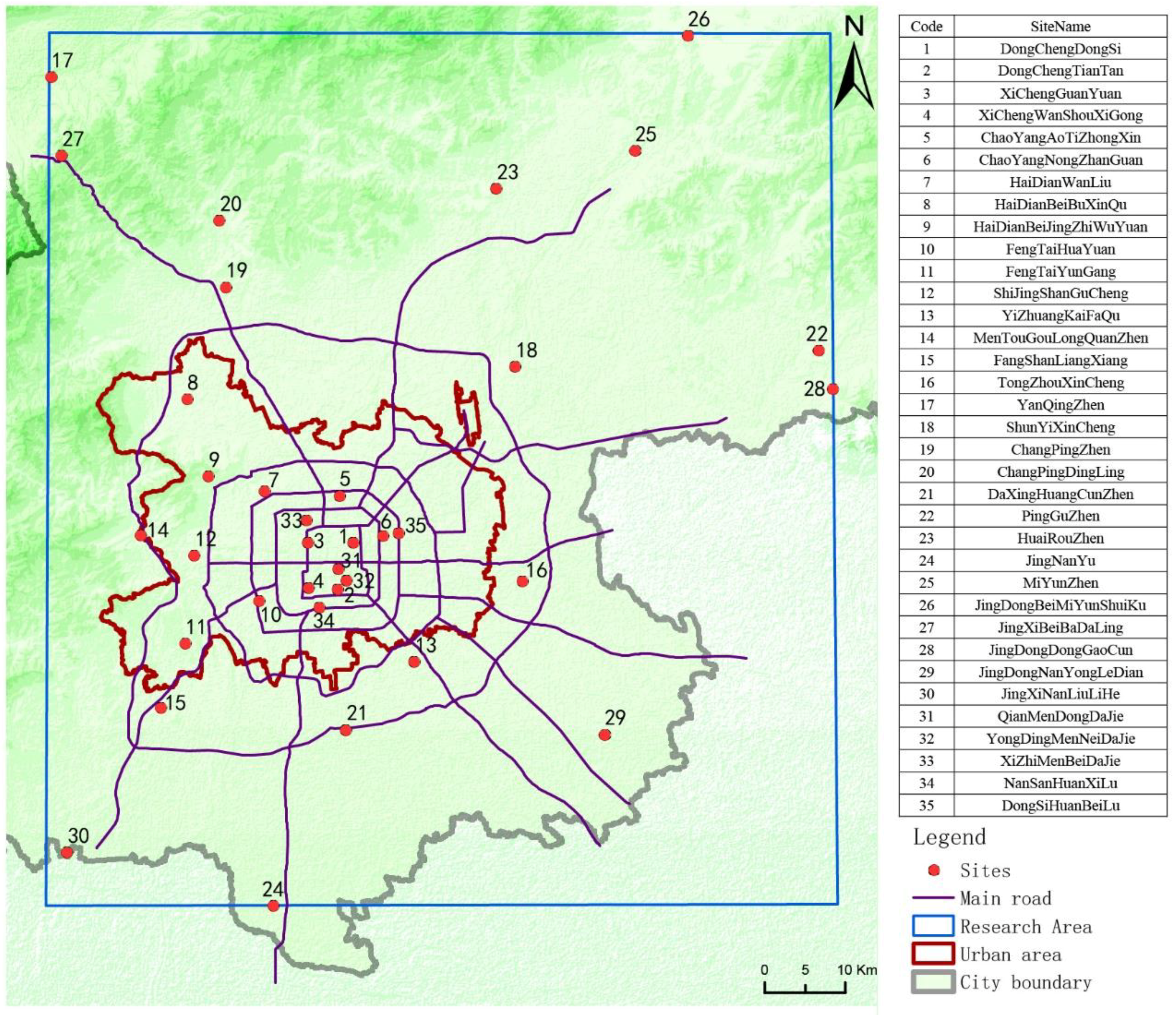
The study area is located in the central and southern parts of Beijing, and is a rectangular range built on the four corners of the 35 environmental monitoring sites in Beijing. It is located at 115.9–117.1° E, 39.5–40.5° N and has an area of approximately 10,600 km2 (Figure 1). This area includes the urban area of Beijing. The terrain is high in the northwest and low in the southeast. The northwestern region is Yanshan and Taihang Mountains, and the southeastern region is a plain. This area belongs to the northern temperate sub-humid climate, with an average annual rainfall of approximately 600 mm. Due to urbanization in the past decade, the rapid increase in the population, energy consumption, and the number of motor vehicles in Beijing has been accompanied by the frequent outbreak of smog, which poses a serious threat to the health of local residents.
2.2. Data Sources
The input data of this paper are the daily PM2.5 concentration for 31 days (from 1 May 2014 to 31 May 2014) at the 35 monitoring sites in Beijing. The data were obtained from the Beijing Environmental Protection Monitoring Center [28]. The daily average data were calculated by hourly PM2.5 concentration data. In accordance with the scientific principles for the selection of the inspection sites, ChaoYangNongZhanGuan (Site 6), YongDingMenNeiDaJie (Site 32), FengTaiHuaYuan (Site 10) and XiZhiMenBeiDaJie (Site 33) were selected as the four inspection sites in the easterly, southerly, westerly, and northerly directions, respectively. They were used to verify the accuracy at the later stage to compare the interpolation effects of the OK model and the STK model.
2.3. Prediction Model Construction
2.3.1. OK Model
The OK model mainly uses variograms of geographic factors and the structural characteristics of the original data to perform unbiased and linear optimal interpolation estimation of spatial variables. This model can overcome the problem that the interpolation error is difficult to analyze, can theoretically estimate the error point by point, and will not produce the boundary effect of regression analysis. It is an unbiased estimation method of spatial interpolation [29]. The formula for the OK model is
where Z(X) is the estimated value at X; n is the number of monitoring sites; λ is the kriging weight; and Zi is the measured value at Xi.
2.3.2. STK Model
There are two types of STK models: separation models and non-separation models. There are three types of separation models: Bilonick model (BM), Dagum model (DM), and Ma model (MM). There are three types of non-separation models: Cressie-Huang model 1 (CH1), Cressie-Huang model 2 (CH2), and Gneiting model (GM). In addition, some sub-models have corresponding sub-models in the spatial and temporal dimensions and the model’s expression is presented from Equation (2) to Equation (9) [26,27,30]. In this study, the optimal STK model is selected based on the fitting error of six models. The fitting error reflects the matching effect between the time and space position of the sample point and the model fitting surface based on the STK model; the smaller the fitting error, the better the effect of the fitting model.
(1) BM
The model expression is
where is the Spatiotemporal variation function, , and can use the form of spatial variograms, such as the gaussian model, exponential model, spherical model, and linear model; hst is the spatio–temporal distance of spatio-temporal variables, hs is the spatial distance of space-time variables, and ht is the time distance of space and time variables. a is the spatio-temporal geometric anisotropy ratio.
When is selected in the linear model, and are selected in the spherical model, the BM model expression is
where is the spatio-temporal nugget effect, is the spatial dimension coefficient, is the time dimension arch height, is the time dimension variation, and is the spatio-temporal dimension variation.
(2) DM
The model expression is
where is the spatiotemporal variation function, and are the spatio-temporal variograms, respectively. hs is the spatial distance of spatio-temporal variables, and ht is the time distance of spatio-temporal variables. the variogram , is defined as
where , are the spatial and time scale parameter, respectively. , are the spatial smoothing parameters, , are the time smoothing parameters.
(3) MM
The model expression is
where is the spatiotemporal variation function, is the covariance of spatio-temporal variation function, , are the spatial and time variograms, respectively. Similarly, these models can use the gaussian model, exponential model, spherical model, and linear model. hs is the spatial distance of space-time variables, and ht is the time distance of space and time variables.
When is selected the linear model, is selected the spherical model, the MM model expression is
where is the covariance of the spatio-temporal variation function, is the spatio-temporal nugget effect, is the spatial dimension coefficient, is the time dimension arch height, is the time dimension variation, is the spatial distance of space and time variables, and is the time distance of space and time variables.
(4) CH1
The model expression is
where is the spatio-temporal nugget effect, is the covariance of spatio-temporal variation function, is the time dimension arch height, is the spatial dimension coefficient, is the spatial distance of spatio-temporal variables, is the time distance of spatio-temporal variables, and is the spatial variation.
(5) CH2
The model expression is
where is the spatio-temporal nugget effect, is the covariance of spatio-temporal variation function, is the time dimension arch height, is the spatial dimension coefficient, is the spatio-temporal scale parameter, is spatial distance of spatio-temporal variables, and is the time distance of spatio-temporal variable, and is the spatial variation.
(6) GM
The model expression is
where, is the covariance of spatio-time variation function, is the time scale parameter, is the spatial scale parameter, , are smoothing parameter, and is the spatial dimension.
2.4. Model Error Analysis
In this study, we used the cross-examination method to compare the simulation performance of two different interpolation methods, OK and STK. The principle is to first assume that the PM2.5 concentration at the inspection site is unknown. Then, the known data from the surrounding sites are used for prediction. Through the analysis of the error between the predicted and measured values, the optimal PM2.5 exposure simulation prediction method is selected. The error analysis was conducted using four indicators, i.e., the minimum error (MINE), maximum error (MAXE), root mean square error (RMSE) and mean absolute error (MAE). MINE and MAXE were used to calculate the minimum error and the maximum error, respectively. RMSE was used to indicate the relative estimation error, and MAE was used to estimate the possible error range of the prediction value.
where n is the number of inspection sites, Zi is the measured PM2.5 value of the i-th station, and Z(Xi) is the simulated prediction value of the i-th station.
2.5. Daily Average Concentration Calculation
In this study, the spatial–temporal distribution characteristics of the PM2.5 daily average concentration in Beijing in May 2014 were analyzed using two methods: The daily average concentration based on site statistics and the daily PM2.5 exposure value of the whole region based on spatial statistics. The equations are
where and are the daily average concentration based on the site statistics and the daily average concentration based on the spatial statistics, respectively, and are the number of monitoring sites and the number of grids after the interpolation, respectively, and and are the i-th monitoring site and the -th grid value, respectively.
3. Results and Analysis
3.1. Comparison of STK Models
Before entering data into the STK model, the raw input PM2.5 concentration data were log transformed to approach a normal distribution. The time resolution, time step, spatial resolution, and the spatial step were set as 1 day, 7 days, 1 km, and 10 km, respectively. Next, the three separation models, BM, DM, and MM, and the three non-separation models, CH1, CH2, and GM, were used for model fitting. The parameters of each model are shown in Table 1. The models are ranked as follows based on their fitting error(f): BM (0.00648) < CH1 (0.00654) < DM (0.00751) < MM (0.01589) < CH2 (0.01783) < GM (0.05317). The fitting error of the BM model is the smallest, indicating that the BM model has the best fitting effect. The fitting effect of this model is shown in Figure 2. Therefore, the BM model was selected as the STK fitting model for the daily PM2.5 exposure.
3.2. Comparison of OK and STK
Using the BM model of STK, the PM2.5 daily average concentration data for May 2014 were spatial–temporally interpolated. The results of the PM2.5 STK simulation prediction of the study area with a time resolution of 1 day and a spatial resolution of 1 km were obtained. Error analysis was carried out on the monitoring data of the four inspection sites and the simulated prediction values. The OK model used the monitoring data from the same site for simulation prediction and accuracy verification. The following is evident in Table 2: The MINE values of the OK and STK models are the same, both of which are 0.01, indicating that the minimum estimation errors of the two interpolation methods are both small. The MAXE, MAE, and RMSE values are 32.57, 7.91, and 10.70 for the OK model, and 30.45, 6.14, and 8.90, respectively, for the STK model. The three errors of the STK model are obviously smaller than those of the OK model, indicating that the PM2.5 simulation prediction results of the STK model are clearly better than those of the OK model. The STK model is a more accurate interpolation model.
4. Discussion
4.1. Overall Quantity Characteristics of PM2.5
The spatial–temporal distribution of PM2.5 daily average concentrations in Beijing in May 2014 was obtained based on the prediction of the STK model. To better analyze the spatial–temporal differentiation characteristics of PM2.5 air quality in Beijing, we adopted the national standards implemented in China in 2016, i.e., the GB 3095-2012 Ambient Air Quality Standards [31]. China ‘s GB 3095-2012 standard behind the standard of WHO [32]; however, China ‘s standard is consistent with the target WHO Interim target-1. The PM2.5 air quality grade in GB 3095-2012, daily PM2.5 exposure criteria, and its health impacts are shown in Table 3. According to different dailyPM2.5 exposure values, the air quality of PM2.5 was classified into six grades, i.e., good (0–35 μg m−3), moderate (35–75 μg m−3), lightly polluted (75–115 μg m−3), moderately polluted (115–150 μg m−3), heavily polluted (150–250 μg m−3), and severely polluted (250–500 μg m−3). Based on this standard, the spatial–temporal characteristics of daily PM2.5 exposure in Beijing in May 2014 were further evaluated.
Using the site averages as the city’s daily average concentration values in Beijing and based on the results of STK interpolation, we calculated the daily average concentration in all spatial ranges in the study area in May 2014 as the daily PM2.5 exposure in the city. As shown in Table 3, in May 2014, the city’s daily air quality grades of PM2.5 in Beijing were mainly good and moderate, accounting for 29.03% and 41.94%, respectively, of the total number of days. Pollution was mainly lightly polluted and moderately polluted, accounting for 25.81% and 3.23%, respectively, of the total number of days, while heavily polluted and severely polluted did not occur. The overall air quality in this period was mainly good and moderate, and the air quality was relatively good.
4.2. Time Variation Characteristics of PM2.5
In this paper, the daily PM2.5 exposure value based on the statistical data of 35 monitoring sites and the regional daily PM2.5 exposure value of the spatial statistics based on the STK interpolation were calculated. The comparison shows the following: There are certain differences between the two calculation results of the daily PM2.5 exposure. The daily PM2.5 exposure based on the site average is slightly lower than the regional average, but the overall trend of the two methods remains consistent. As shown in Figure 3, the daily PM2.5 exposure in Beijing in May 2014 had good continuity in the temporal domain, showing a cyclical trend of a decrease and then an increase followed by another decrease before an increase, which may be due to the change of wind speed and wind direction in Beijing in May; the PM2.5 concentration is high (e.g., 22 May) when the wind speed is weak and wind direction is south. conversely, the PM2.5 concentration declines when the wind speed is strong and wind direction is north (e.g., 27 May). The daily PM2.5 exposure was the highest on the 1st, 19th, 21st, 22nd, and 31st, all higher than 100 μg m−3. The daily PM2.5 exposure was the lowest on the 2nd, 4th, 5th, 11th, 14th, 26th, and 28th, all less than 30 μg m−3.
4.3. Spatial Variation Characteristics of PM2.5
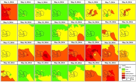
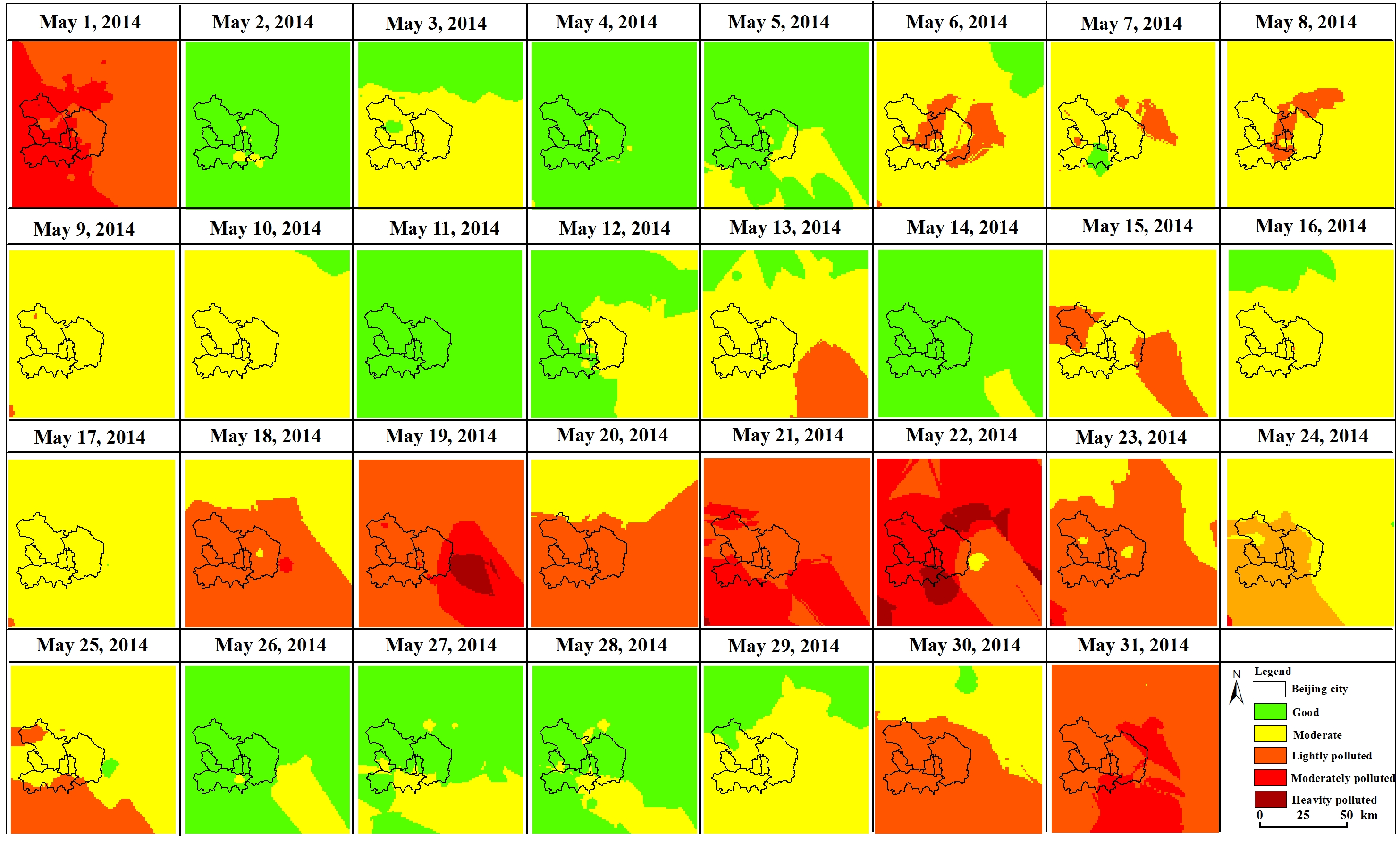
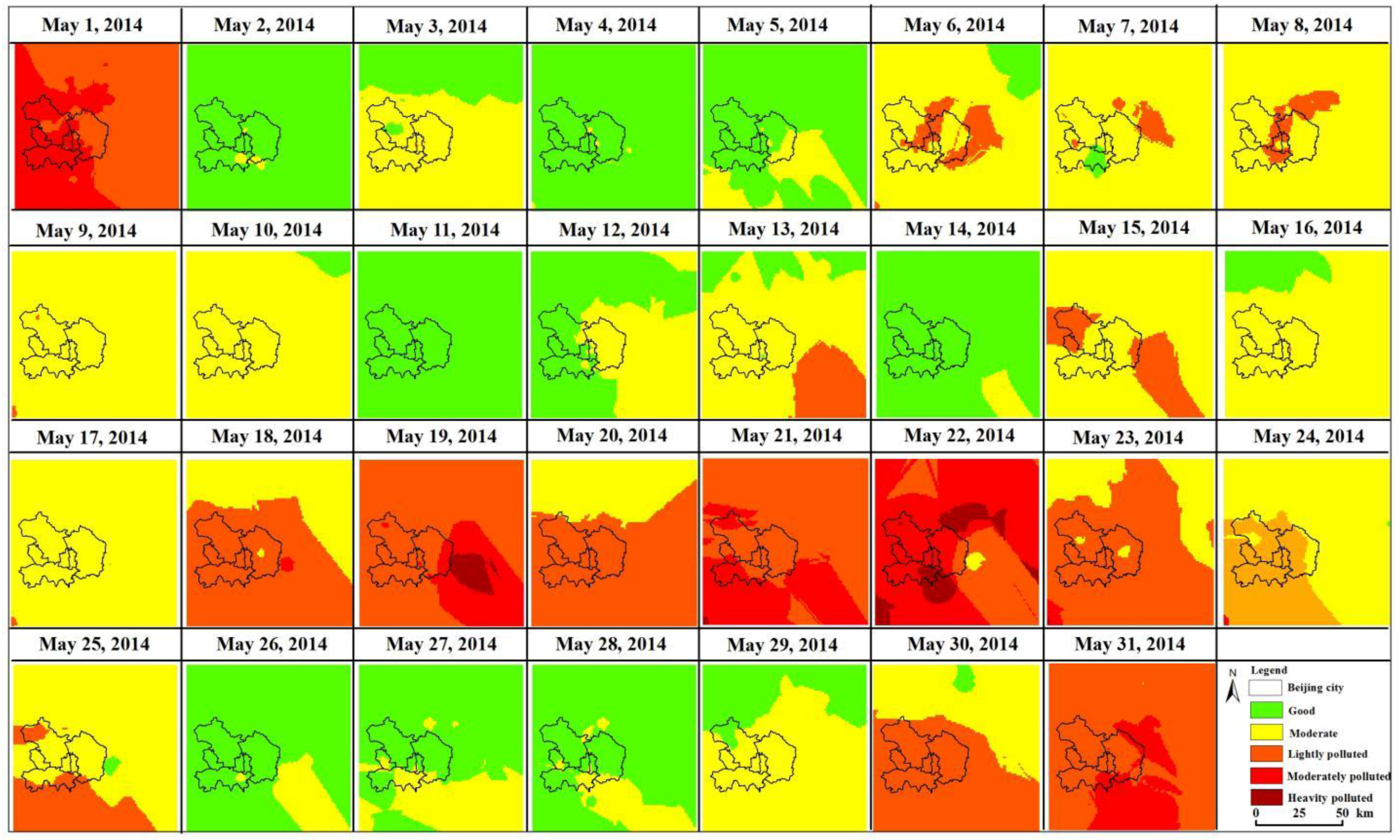
Based on the results of the STK interpolation, the spatial distribution characteristics of daily PM2.5 exposure in Beijing in May 2014 are shown in Figure 4. The PM2.5 exposure also had good spatial continuity, and there was a large spatial heterogeneity between different regions. The areas with higher PM2.5 exposure were mainly concentrated in the urban areas of Beijing. Light and moderate pollution occurred mainly on the 1 May. The northeast and southeast areas were mainly covered by moderate and heavy pollution on the 21st and 31st, respectively, and the remaining areas were covered by light pollution. Local light pollution appeared on the 6th, 7th, 8th, 13th, 15th, and 25th, and the rest of the areas had good air quality. On the 18th, 20th, 23rd, and 30th, moderate pollution covered mainly the southern area. In addition, on the 19th and 22nd, different levels of heavy pollution occurred in the main downtown area and its surrounding areas.
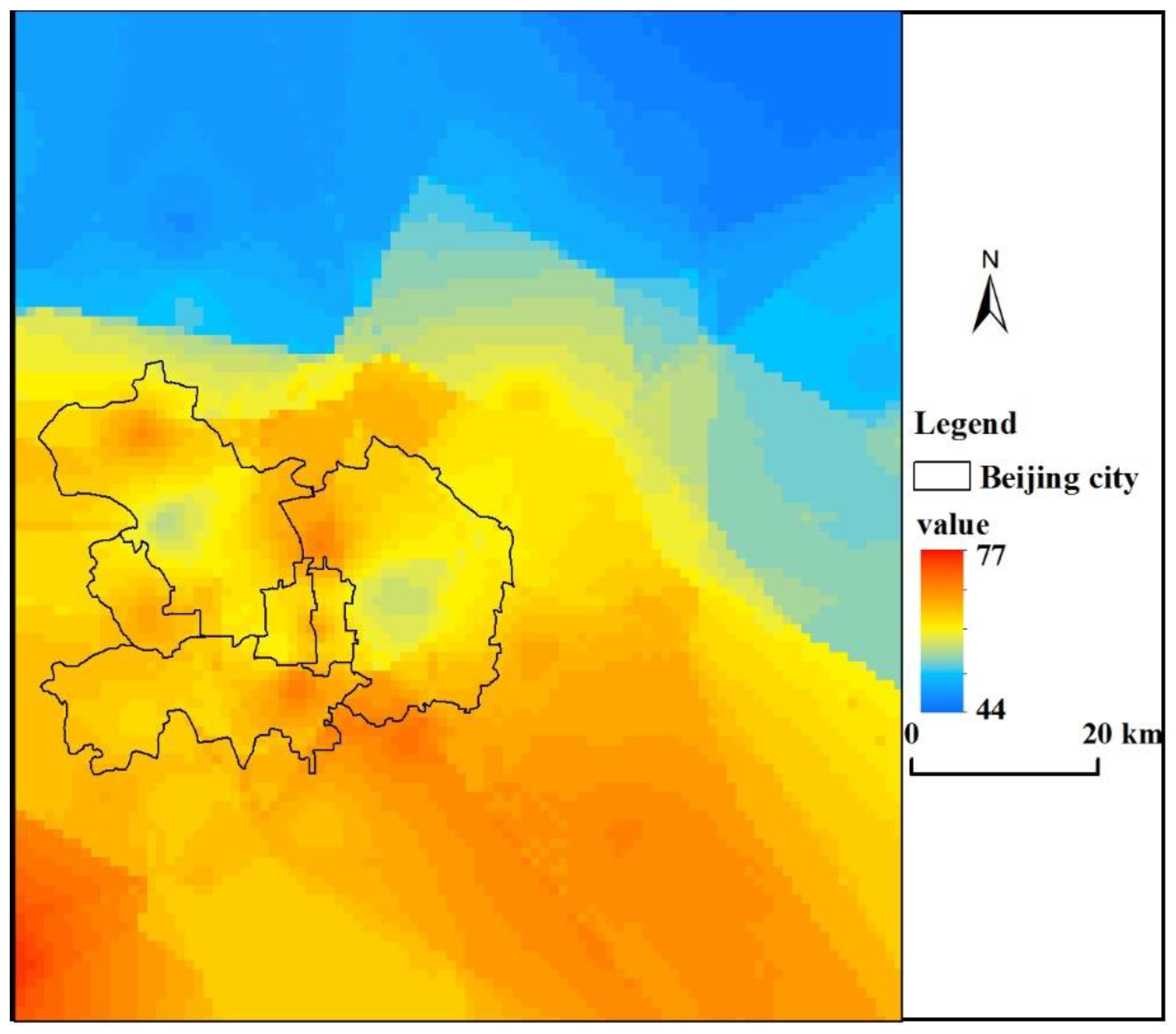
The spatial distribution characteristics of the cumulative mean of the daily PM2.5 exposure in Beijing in May 2014 are shown in Figure 5. The 31-day cumulative mean had good continuity in space, showing a general trend of being higher in the south and lower in the north. From the north to the south, there was a gradual transition from low to high exposure. In the southwestern part of the study area, the cumulative daily PM2.5 exposure concentration of PM2.5 was the highest, indicating that the area had been under a high PM2.5 exposure concentration of pollution for a long time. According to previous studies [33], the spatial distribution feature of PM2.5 exposure in Beijing may be related to topography and traffic emission. West of Beijing is Xishan Mountains, part of the Taihang Mountain; north of the city is Jundu Mountain, part of the Yanshan Mountains; surrounding the Beijing plain, these two mountains form a semicircular arc, extending to the southeast. Daily emissions from Beijing disperse towards the opening of the mountain arc, over the flat plain. Moreover, the ring road traffic in Beijing has further aggravated spatial agglomeration characteristics of PM2.5. The cumulative concentration of PM2.5 exposure was also high in the southeast, posing a great hazard in this region. The PM2.5 cumulative exposure concentration was low in the northern area, and the overall air quality was good.
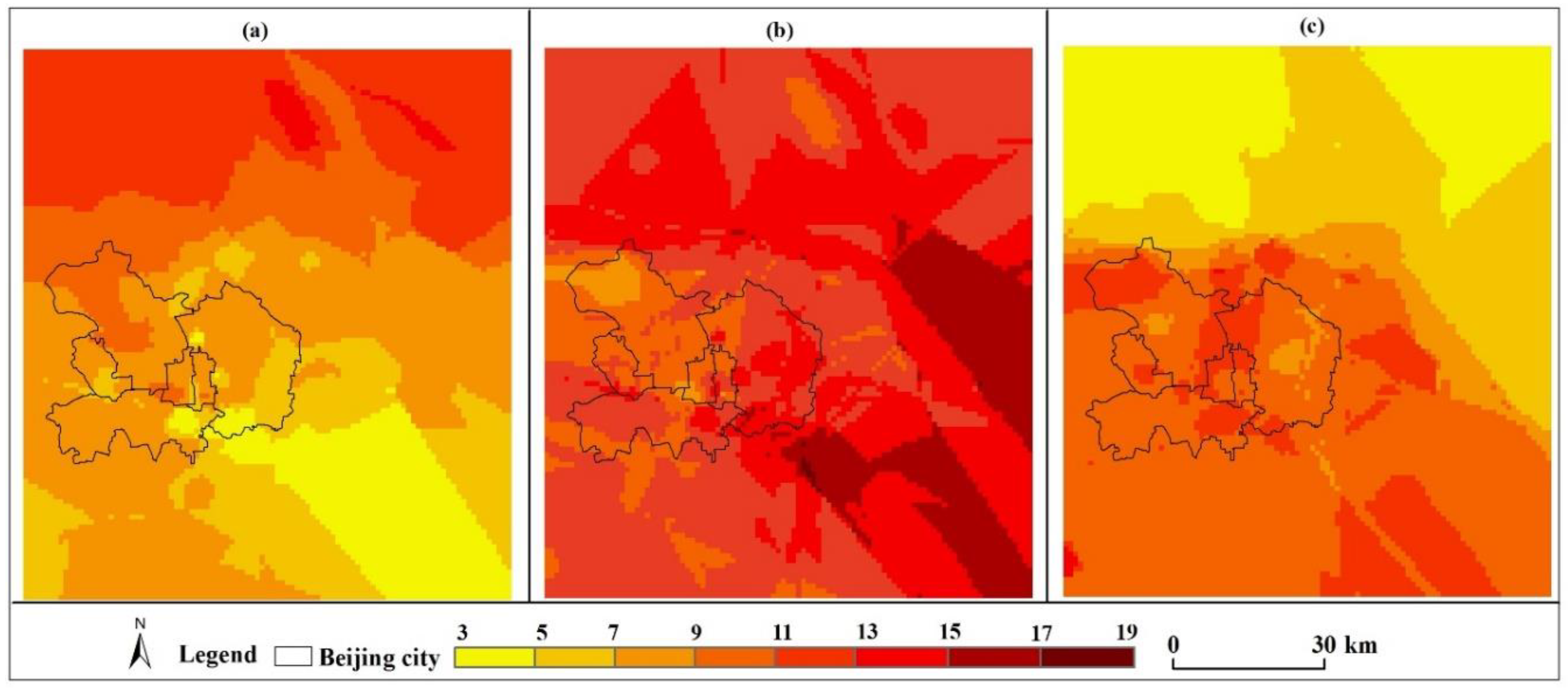
Based on the grading results of the daily PM2.5 exposure concentration after STK interpolation, the cumulative duration of the air quality of the daily PM2.5 exposure in Beijing at good, moderate, and polluted (including lightly polluted, moderately polluted, heavily polluted, and severely polluted grades) grades was calculated. As shown in Figure 6, in May 2014, there was a certain degree of heterogeneity in the cumulative duration of different PM2.5 air quality grades in Beijing. The cumulative duration of good air quality was 3 to 14 days, and the region with the maximum cumulative duration was in the north of the study area. The cumulative duration for moderate air quality was relatively long, ranging from 8 to 14 days, and the area with the largest cumulative duration was in the southeast of the study area. The cumulative duration for air quality in the polluted grades was 4 to 14 days, and the area with the longest cumulative duration was in the southwest of the study area.
5. Conclusions and Implications
Based on the daily average concentration of PM2.5 in May 2014 in Beijing, we discussed the fitting effect of six different STK models, performed comparison analysis of the errors between STK and OK, and analyzed the spatial–temporal distribution characteristics of the daily PM2.5 exposure in Beijing based on the optimal interpolation model. The main conclusions are as follows:
- (1)
- The comparison of the fitting accuracy of STK for the three separation models, BM, DM, and MM, and the three non-separation models, CH1, CH2, and GM, shows that the fitting error of the BM model is the smallest, indicating the best fitting effect for the prediction model of daily PM2.5 exposure to be STK.
- (2)
- The cross-examination results show that the minimum errors between OK and STK are close. However, the STK fitting errors are significantly lower than those of OK, indicating that the prediction effect of STK for PM2.5 is significantly better than that of OK. The STK model is a more accurate prediction model for daily PM2.5 exposure in Beijing.
- (3)
- From the STK prediction results simulated by the BM model, the daily PM2.5 exposure concentration in Beijing has good continuity in both time and space and also has considerable heterogeneity. In May 2014, the overall air quality of PM2.5 in Beijing was good, and the air quality showed a cyclical trend of decreasing before increasing followed by another decrease prior to an increase. During this period, heavy pollution occurred only in a few areas, and the overall spatial distribution characteristics were low pollution in the north and high pollution in the south, with the highest daily PM2.5 exposure concentration in the southwest.
- (4)
- In May 2014, there was some heterogeneity in the cumulative exposure duration of PM2.5 at different air quality grades in Beijing. The region with the longest cumulative duration of good air quality was in the northern part of the study area. The region with the longest cumulative duration of moderate air quality was in the southeast of the study area. The region with the longest cumulative duration of polluted air quality was in the southwest of the study area.
In this paper, we studied the spatial–temporal distribution characteristics of daily PM2.5 exposure in Beijing based on the STK model. Compared with the OK model, the problem of the lack of interpolation in the temporal dimension in the traditional interpolation method is solved. However, like the OK model, this method is also based on the limited monitoring sites discretely distributed in space for interpolation simulation and fails to consider the supporting simulation role of other relevant factors. It cannot achieve high-precision PM2.5 exposure concentration estimation and cannot obtain the internal difference characteristics of small areas. In addition, the hourly level model cannot be realized due to a large amount of computation and the limit of the model tool in our research now. In future research, the hourly PM2.5 exposure will be achieved in higher spatial and temporal accuracy by increasing the time precision to the hour level or combining with other relevant factors.
Author Contributions
J.L. designed and implemented the data analysis methods and wrote the manuscript. A.Z. and W.C. supervised the data analysis, participated in writing and revising the manuscript. M.L. assisted with the data analysis and manuscript preparation.
Funding
This research was funded by the National Key Research and Development Program of China (Grant No. 2017YFB0503500), the Strategic Priority Research Program of the Chinese Academy of Sciences (Grant No. XDA19040402), National Natural Science Foundation of China (Grant No. 41421001, 41471414, 41201412), Featured Institute Construction Services Program (Grant No. TSYJS03) and Basic Science-technological Special Working (Grant No. 2015FY210600).
Conflicts of Interest
The authors declare no conflict of interest.
References
- Fang, C.L.; Liu, H.M.; Li, G.D. International progress and evaluation on interactive coupling effects between urbanizationand the eco-environment. J. Geogr. Sci. 2016, 26, 1081–1116. [Google Scholar] [CrossRef]
- Chen, Z.; Wang, J.N.; Ma, G.X.; Zhang, Y.S. China tackles the health effects of air pollution. Lancet 2013, 382, 1959–1960. [Google Scholar] [CrossRef]
- Chan, C.K.; Yao, X. Air pollution in mega cities in China. Atmos. Environ. 2008, 42, 1–42. [Google Scholar] [CrossRef]
- Wang, Z.B.; Fang, C.L.; Guang, X.U.; Pan, Y. Spatial-temporal characteristics of the PM2.5 in China in 2014. Acta Geogr. Sin. 2015, 70, 1720–1734. [Google Scholar] [CrossRef]
- Han, L.; Zhou, W.; Li, W. Growing Urbanization and the Impact on Fine Particulate Matter (PM2.5) Dynamics. Sustainability 2018, 10, 1696. [Google Scholar] [CrossRef]
- Kan, H.; Chen, R.; Tong, S. Ambient air pollution, climate change, and population health in China. Environ. Int. 2012, 42, 10–19. [Google Scholar] [CrossRef] [PubMed]
- Guan, D.B.; Su, X.; Zhang, Q.; Peters, G.P.; Liu, Z.; Lei, Y.; He, K.B. The socioeconomic drivers of China’s primary PM2.5 emissions. Environ. Res. Lett. 2014, 9. [Google Scholar] [CrossRef]
- Jung, J.; Lee, H.; Kim, Y.J.; Liu, X.; Zhang, Y.; Gu, J.; Fan, S. Aerosol chemistry and the effect of aerosol water content on visibility impairment and radiative forcing in Guangzhou during the 2006 pearl river delta campaign. J. Environ. Manag. 2009, 90, 3231–3244. [Google Scholar] [CrossRef] [PubMed]
- Tie, X.; Wu, D.; Brasseur, G. Lung cancer mortality and exposure to atmospheric aerosol particles in Guangzhou, China. Atmos. Environ. 2009, 43, 2375–2377. [Google Scholar] [CrossRef]
- Wang, Z.; Li, Y.T.; Chen, T.; Zhang, D.; Feng, S.; Pan, L. Spatial-temporal characteristics of PM2.5 in Beijing in 2013. Acta Geogr. Sin. 2015, 70, 110–120. [Google Scholar] [CrossRef]
- Landrigan, P.J.; Fuller, R.; Acosta, N.J.R.; Adeyi, O.; Arnold, R.; Basu, N.N.; Baldé, A.B.; Bertollini, R.; Bose-O’Reilly, S.; Boufford, J.I.; et al. The lancet commission on pollution and health. Lancet 2017, 391, 462–512. [Google Scholar] [CrossRef]
- Wang, Y.S.; Li, Y.; Wang, L.L.; Liu, Z.R.; Ji, D.S.; Tang, G.Q.; Zhang, J.K.; Sun, Y.; Hu, B.; Xin, J.Y. Mechanism for the formation of the January 2013 heavy haze pollution episode over central and eastern China. Sci. China Earth Sci. 2014, 57, 14–25. [Google Scholar] [CrossRef]
- Yang, Y.; Lu, X.S.; Li, D.L. Research progress of environmental health risk assessment in China. J. Environ. Health 2014, 31, 357–363. [Google Scholar] [CrossRef]
- Li, L.; Zhang, J.; Qiu, W.; Wang, J.; Fang, Y. An ensemble spatiotemporal model for predicting PM2.5 concentrations. Int. J. Environ. Res. Public Health 2017, 14, 549. [Google Scholar] [CrossRef] [PubMed]
- Yang, Y.; Christakos, G. Spatiotemporal characterization of ambient PM2.5 concentrations in Shandong province (China). Environ. Sci. Technol. 2015, 49, 13431–13438. [Google Scholar] [CrossRef] [PubMed]
- Guo, W.B.; Zhang, Y.; Cai, Y.W. Measurement of residents’ daily travel air pollution exposure and its mechanism: A case study of suburban communities in Beijing. Geogr. Res. 2015, 34, 1310–1318. [Google Scholar] [CrossRef]
- Wang, Q.; Dong, X.Y.; Gao, S.H.; Wu, L.P.; Zhu, H.J. Advances of research on environmental pollution exposure assessment. J. Environ. Health 2016, 33, 1025–1030. [Google Scholar] [CrossRef]
- Gilliland, F.; Avol, E.; Kinney, P.; Jerrett, M.; Dvonch, T.; Lurmann, F.; Buckley, T.; Breysse, P.; Keeler, G.; de Villiers, T.; et al. Air pollution exposure assessment for epidemiologic studies of pregnant women and children: Lessons learned from the centers for children’s environmental health and disease prevention research. Environ. Health Perspect. 2005, 113, 1447–1454. [Google Scholar] [CrossRef] [PubMed]
- Wu, J.S.; Xie, W.D.; Li, J.C. Application of landuse regression models in spatial-temporal differentation of air pollution. Environ. Sci. 2016, 37, 413–419. [Google Scholar] [CrossRef]
- Hoek, G.; Beelen, R.; Hoogh, K.D.; Vienneau, D.; Gulliver, J.; Fischer, P.; Briggs, D. A review of land-use regression models to assess spatial variation of outdoor air pollution. Atmos. Environ. 2008, 42, 7561–7578. [Google Scholar] [CrossRef]
- Clench-Aas, J.; Bartonova, A.; Bohler, T.; Gronskei, K.E.; Sivertsen, B.; Larssen, S. Air pollution exposure monitoring and estimating. Part I. Integrated air quality monitoring system. J. Environ. Monit. 1999, 1, 313–319. [Google Scholar] [CrossRef] [PubMed]
- Jerrett, M.; Arain, A.; Kanaroglou, P.; Beckerman, B.; Potoglou, D.; Sahsuvaroglu, T.; Morrison, J.; Giovis, C. A review and evaluation of intraurban air pollution exposure models. J. Expos. Anal. Environ. Epidemiol. 2004, 15, 185. [Google Scholar] [CrossRef] [PubMed]
- Mulholland, J.; Butler, A.; Wilkinson, J.; Russell, A.; Tolbert, P. Temporal and spatial distributions of ozone in Atlanta: Regulatory and epidemiologic implications. J. Air Waste Manag. Assoc. 1998, 48, 418–426. [Google Scholar] [CrossRef] [PubMed]
- Yun, H.; He, L.Y.; Huang, X.F.; Lan, Z.J.; Li, X.; Zeng, L.W. Characterising seasonal variation and spatial distribution of PM2.5 species in Shenzhen. Environ. Sci. 2013, 34, 1245–1251. [Google Scholar] [CrossRef]
- Zhao, C.X.; Wang, Y.Q.; Wang, Y.J.; Zhang, H.L.; Zhao, B.Q. Temporal and spatial distribution of PM2.5 and PM10 pollution status and the correlation of particulate matters and meteorological factors during winter and spring in Beijing. Environ. Sci. 2014, 35, 418–427. [Google Scholar] [CrossRef]
- Yang, Y.; Christakos, G.; Guo, M.W.; Xiao, L.; Huang, W. Space-time quantitative source apportionment of soil heavy metal concentration increments. Environ. Pollut. 2017, 223, 560–566. [Google Scholar] [CrossRef] [PubMed]
- Yang, Y.; Mei, Y.; Zhang, C.T.; Liao, X. Spatio-temporal modeling and prediction of soil heavy metal based on spatio-temporal Kriging. Trans. Chin. Soc. Agrc. Eng. 2014, 30, 249–255. [Google Scholar] [CrossRef]
- Beijing Environmental Protection Monitoring Center. 2014. Available online: http://www.bjmemc.com.cn (accessed on 1 December 2016).
- Liu, F.R.; Hung, M.J.; Kuo, J.Y.; Liang, H.H. Using GIS and kriging to analyze the spatial distributions of the health risk of indoor air pollution. J. Geosci. Environ. Prot. 2015, 3, 20–25. [Google Scholar] [CrossRef]
- Yang, Y.; Wu, J.; Christakos, G. Prediction of soil heavy metal distribution using Spatiotemporal Kriging with trend model. Ecol. Indic. 2015, 56, 125–133. [Google Scholar] [CrossRef]
- Ministry of Environmental Protection. Ambient Air Quality Standards (GB 3095-2012). 2012. Available online: http://english.mep.gov.cn/Resources/standards/Air_Environment/quality_standard1/201605/W020160511506615956495.pdf (accessed on 1 January 2016).
- World Health Organization. WHO Air Quality Guidelines for Particulate Matter, Ozone, Nitrogen Dioxide and Sulfur Dioxide; Global Update Summary of Risk Assessment; World Health Organization: Geneva, Switzerland, 2006. [Google Scholar]
- Zhang, A.; Qi, Q.; Jiang, L.L.; Zhou, F.; Wang, J.F. Population exposure to PM2.5 in the urban area of Beijing. PLoS ONE 2013, 5, e63486. [Google Scholar] [CrossRef] [PubMed]
Figure 1.
Geographic location of the study area.

Figure 2.
Spatial–temporal fitting effect of PM2.5 concentration for the BM model.
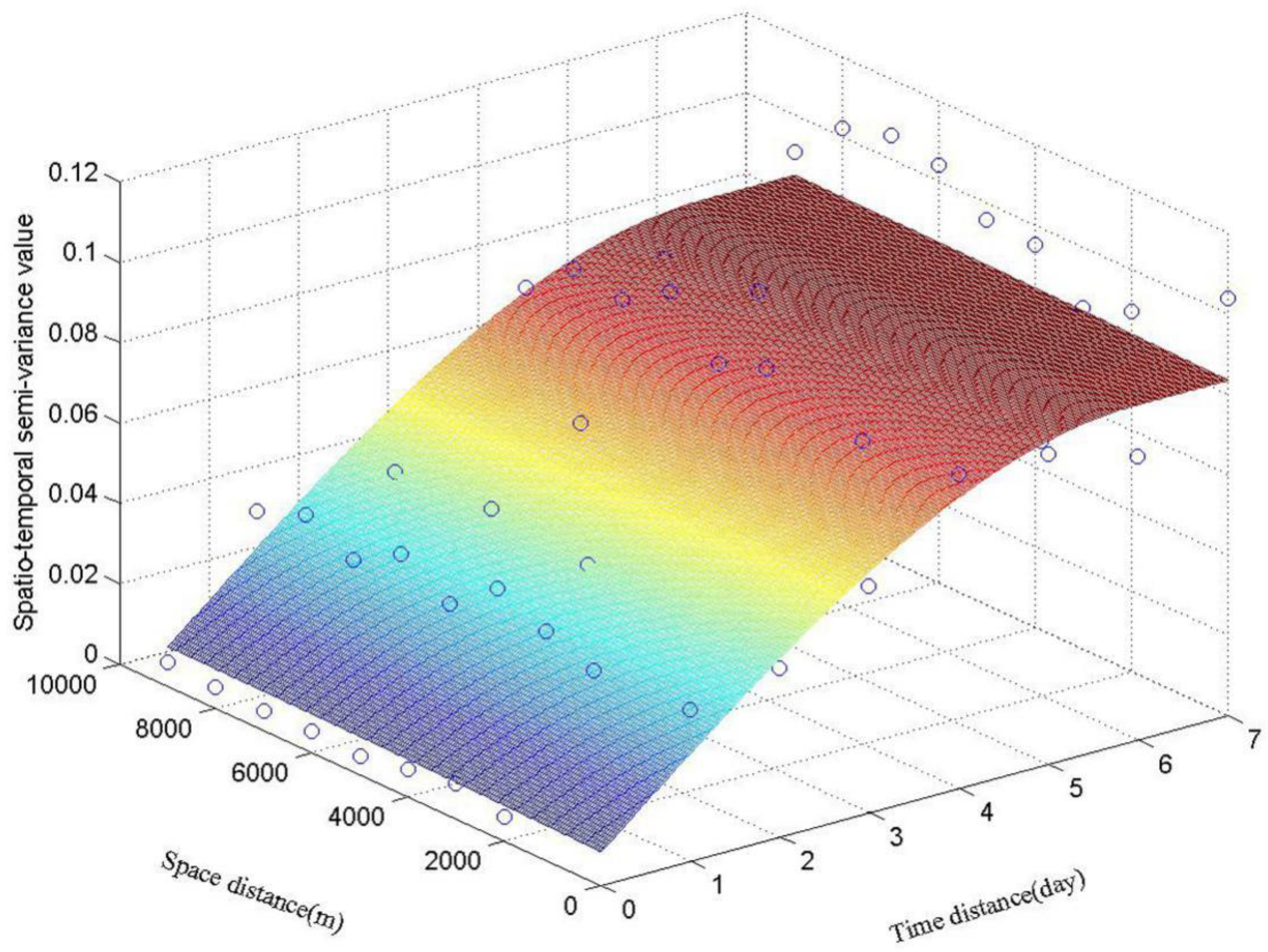
Figure 3.
Daily PM2.5 exposure in Beijing in May 2014.
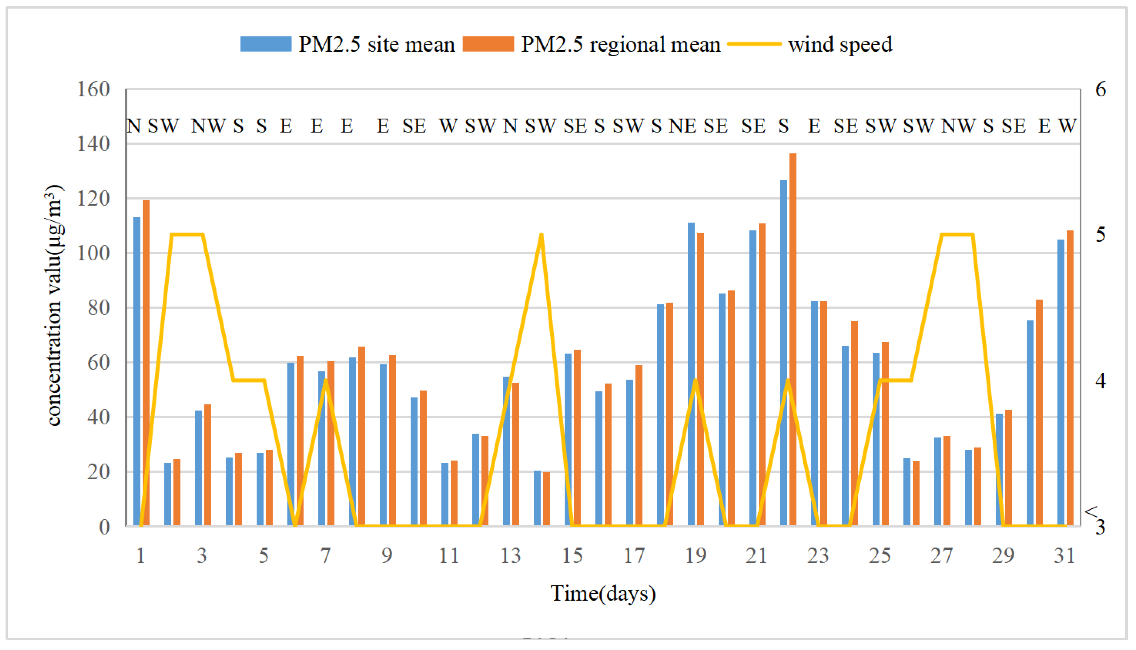
Figure 4.
Spatial distribution of PM2.5 exposure concentration in Beijing in May 2014.

Figure 5.
Average of the 31-day cumulative daily exposure concentration of PM2.5 in Beijing in May 2014.
Figure 5.
Average of the 31-day cumulative daily exposure concentration of PM2.5 in Beijing in May 2014.

Figure 6.
Spatial distribution of the cumulative duration of PM2.5 in Beijing with air quality at good (a), moderate (b), and polluted (c) grades.
Figure 6.
Spatial distribution of the cumulative duration of PM2.5 in Beijing with air quality at good (a), moderate (b), and polluted (c) grades.


Table 1.
Parameters and errors of different variogram Models of PM2.5 daily average concentration in Beijing.
Table 1.
Parameters and errors of different variogram Models of PM2.5 daily average concentration in Beijing.
| Model | Parameters and Errors | |||||||
|---|---|---|---|---|---|---|---|---|
| f | C0 | Cs | Ct | at | Cst | ast | a | |
| BM | 0.00648 | 0.0082 | 8.1187 × 10⁻⁸ | 5.9684 | 0.0751 | 0.0008 | 7005.2376 | 1325.1108 |
| f | Cs | as | βs | Ct | at | βt | ||
| DM | 0.00751 | 83.9718 | 0.0137 | 2.2016 | 11.1526 | 0.3023 | 1.2126 | |
| f | σ | C0 | Cs | Ct | at | |||
| MM | 0.01589 | 0.3114 | 0.1387 | 0.7331 | 3.4125 | 3.2701 | ||
| f | σ | C0 | Ct | Cs | a1 | a2 | ||
| CH1 | 0.00654 | 0.3221 | 0.0194 | 0.0998 | 1.0 × 10⁻⁷ | 7.8735 × 10⁻⁶ | 0.2981 | |
| f | σ | C0 | Ct | Cs | Cst | a1 | a2 | |
| CH2 | 0.01783 | 0.2121 | 0.0452 | 0.8843 | 1.6224 × 10⁻⁹ | .2.3828×10−10 | 1.3781 × 10⁻⁶ | 0.1961 |
| f | σ | α | β | c | γ | d | ||
| GM | 0.05317 | 0.2582 | 1.3093 | 0.6905 | 1.0176 | 1.9941 | 0.7224 | |
Table 2.
Comparison of error analysis between spatial–temporal kriging and ordinary kriging.
| Ordinary Kriging (OK) | Spatial–Temporal Kriging (STK) | ||||||
|---|---|---|---|---|---|---|---|
| MAXE | MINE | MAE | RMSE | MAXE | MINE | MAE | RMSE |
| 32.57 | 0.01 | 7.91 | 10.70 | 30.45 | 0.01 | 6.14 | 8.90 |
Table 3.
PM2.5 air quality grades and their proportions in Beijing in May 2014.
| Air Quality Grade | Number of Days | Date | Proportion |
|---|---|---|---|
| Good | 9 | 2, 4, 5, 11, 12, 14, 26, 27, 28 | 29.03% |
| Moderate | 13 | 3, 6, 7, 8, 9, 10, 13, 15, 16, 17, 24, 25, 29 | 41.94% |
| Lightly polluted | 8 | 1, 18, 19, 20, 21, 23, 30, 31 | 25.81% |
| Moderately polluted | 1 | 22 | 3.23% |
© 2018 by the authors. Licensee MDPI, Basel, Switzerland. This article is an open access article distributed under the terms and conditions of the Creative Commons Attribution (CC BY) license (http://creativecommons.org/licenses/by/4.0/).
Share and Cite
MDPI and ACS Style
Lin, J.; Zhang, A.; Chen, W.; Lin, M. Estimates of Daily PM2.5 Exposure in Beijing Using Spatio-Temporal Kriging Model. Sustainability 2018, 10, 2772. https://doi.org/10.3390/su10082772
AMA Style
Lin J, Zhang A, Chen W, Lin M. Estimates of Daily PM2.5 Exposure in Beijing Using Spatio-Temporal Kriging Model. Sustainability. 2018; 10(8):2772. https://doi.org/10.3390/su10082772
Chicago/Turabian StyleLin, Jinhuang, An Zhang, Wenhui Chen, and Mingshui Lin. 2018. "Estimates of Daily PM2.5 Exposure in Beijing Using Spatio-Temporal Kriging Model" Sustainability 10, no. 8: 2772. https://doi.org/10.3390/su10082772
Note that from the first issue of 2016, this journal uses article numbers instead of page numbers. See further details here.