Proceeding Paper

Generation of Synthetic Hyperspectral Image Cube for Mapping Soil Organic Carbon Using Proximal Remote Sensing †

1
Division of Agricultural Physics, Indian Council of Agricultural Research (ICAR)–Indian Agricultural Research Institute (IARI), New Delhi 110012, India
2
Soil and Water Department, Faculty of Agriculture, Sohag University, Sohag 82524, Egypt
*
Author to whom correspondence should be addressed.
Presented at the 2nd International Electronic Conference on Land (IECL 2025), 4–5 September 2025; Available online: https://sciforum.net/event/IECL2025.
Environ. Earth Sci. Proc. 2025, 36(1), 3; https://doi.org/10.3390/eesp2025036003
Published: 18 November 2025
(This article belongs to the Proceedings of The 2nd International Electronic Conference on Land)

Abstract

The advent of hyperspectral remote sensing represented a breakthrough in the accurate, fast, and non-invasive estimation of important soil fertility parameters. The present study utilizes non-imaging hyperspectral data in the spectral range of 350–2500 nm for estimating soil organic carbon (SOC) content. When partial least squares (PLS) scores were taken as independent variables, support vector machine (SVM) outperformed artificial neural network (ANN) and partial least squares regression (PLSR), achieving an R2 value of 0.83. After pre-processing, the proximal spectral values were spatially interpolated to construct a synthetic hyperspectral image of the experimental fields. By applying the regression model to this synthetic hyperspectral imagery, a high-resolution SOC map showing the variability of organic carbon content in the soil was generated.

1. Introduction

The organic content of soil acts as a strong indicator of soil fertility, which impacts agricultural production and the global carbon cycle. The timely assessment of soil organic carbon is essential for managing its deficiencies to enhance crop growth. However, traditional approaches of laboratory-based SOC estimation are time-consuming and costly with respect to larger sample sizes [1]. Therefore, there exists a growing demand for novel sensor-based approaches for estimating soil fertility parameters without compromising accuracy and precision. The recent advances in hyperspectral remote sensing and the development of sophisticated machine learning regression models have facilitated accurate sensor-based estimation and mapping of SOC. Multiple hyperspectral sensors mounted on different platforms ranging from ground proximal, unmanned aerial vehicles (UAVs), and satellites have proved to be effective in quantifying the organic content in soil using hundreds of high-resolution, contiguous and narrow bands in the spectral range of 350–2500 nm [2]. Kriging-based mapping relies on the spatial distribution of sampling points and provides a statistical interpolation of sparse data collected from the field. In contrast, sensor-based approaches provide the real-time quantitative characterization of soil properties through high-resolution maps using their spectroscopic reflectance. Spectral pre-processing, band selection, and regression modeling, including machine learning and deep learning techniques, play a critical role in extracting information from these SOC response bands [3]. This study introduces an extended kriging method to interpolate spectral data, rather than soil properties, to generate a synthetic hyperspectral image cube for creating soil prediction maps with the aid of machine learning models. Although proximal non-imaging hyperspectral sensors, such as ASD spectroradiometers, provide high-resolution spectral bands for accurate SOC estimation, they cannot deliver high-resolution fertility maps compared with UAV-based or space-borne sensors [4]. Therefore, the underlying novel part of the proposed workflow is to generate imagery showing the spatial distribution of soil fertility using non-imagery spectral data.
Thus, the present study proposes a novel approach to generate a synthetic hyperspectral image cube using the spectral information from a proximal hyperspectral non-imaging sensor. Multiple machine learning models will be evaluated to choose the best one for developing a SOC prediction model. The best prediction model will be applied to a synthetic hyperspectral image for generating a high-resolution SOC map.

2. Materials and Methods

A flowchart showing the major steps adopted for this proposed methodology is shown in Figure 1. The major steps are (i) study area and spectral data collection, (ii) generation of synthetic hyperspectral image, and (iii) optimizing PLS scores and machine learning regression. Each step is explained in detail below.

2.1. Study Area and Spectral Data Collection

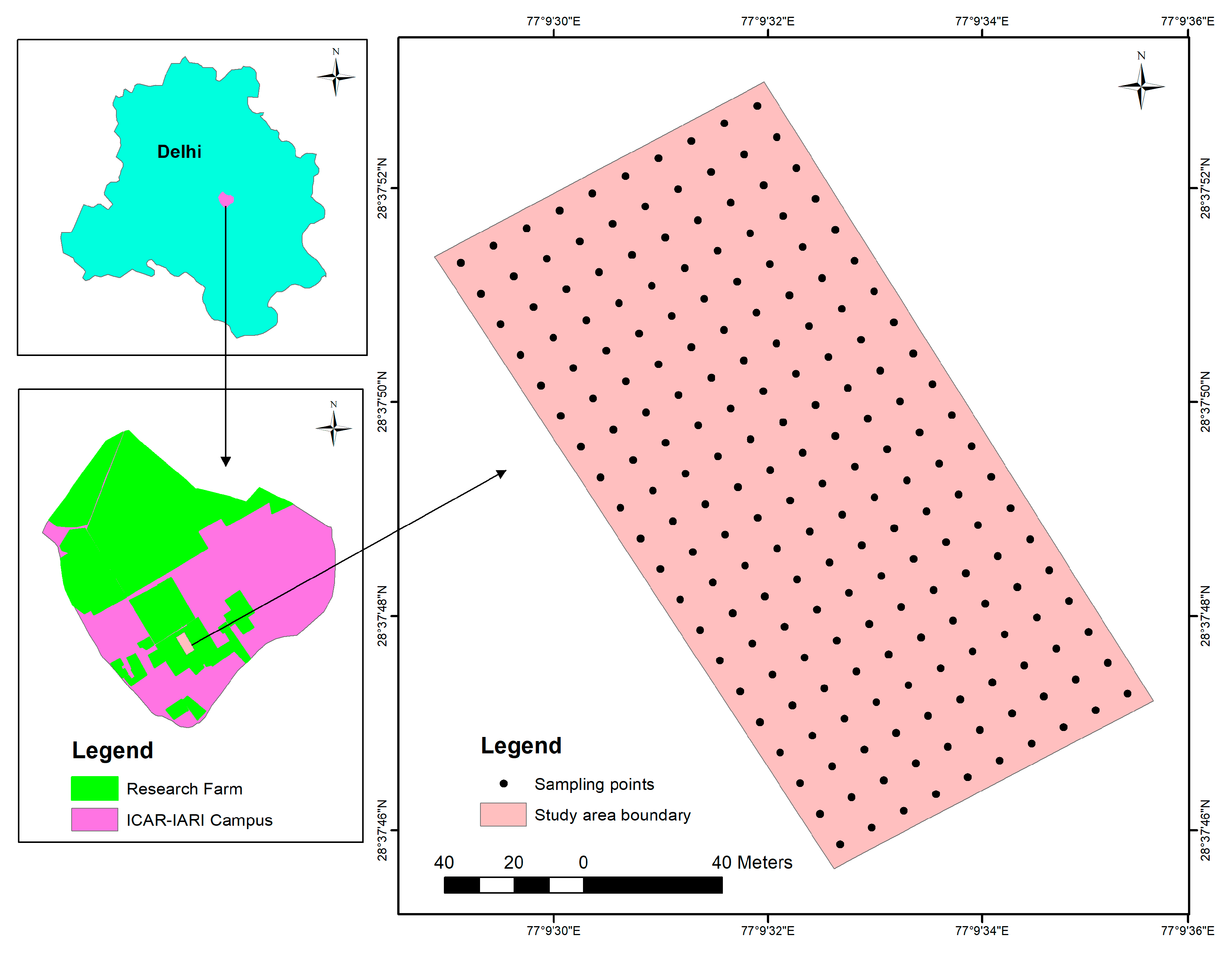
The study was conducted in a 5-acre experimental plot at the research farm of the ICAR—Indian Agricultural Research Institute (IARI), New Delhi, India, situated at geographical coordinates of 28°37′49.81″ N and 77°9′32.00″ E, with an altitude of 228 m above mean sea level. The entire plot was divided into 200 grids, each with a grid dimension of 10 m × 10 m, for soil sampling and spectral data collection. A total of 200 soil samples were collected from the center of each grid at a depth of 0–15 cm. A study area map showing the location of the experimental plot and the spatial distribution of sampling points is shown in Figure 2. A semi-arid climate with hot and dry summers and cold winters exists in the study area. The soil is taxonomically Typic Haplustept, which belongs to the sandy loam textural class. The collected samples were air-dried, finely ground, and passed through a 2 mm pore diameter sieve for chemical analysis in the laboratory. The SOC was determined using the wet chromic acid oxidation technique, also known as the Walkley–Black method [5]. The global Moran’s I index was used to examine the autocorrelation test of the SOC distribution.
The ASD Field Spec 4® Standard-Res portable spectroradiometer (PANalytical Spectral Devices, Inc., Boulder, CO, USA) equipped with a spectral gun was used for in situ collection of spectral data over the 350–2500 nm range at 1 nm spectral intervals. At every sampling location, the spectral gun with a field-of-view of 25° was kept at 1 m above the soil surface at the nadir position for capturing the soil spectra, ensuring the maximum field-of-view was fully covered. The standardization of the sensor was carried out using a white calibration board, called spectralon (Labsphere, North Sutton, NH, USA), made up of barium sulfate, before starting the spectral measurements. The integration time was fixed at 100 milliseconds. The spectral pre-processing involves the following steps: (i) splice correction, (ii) removal of marginal bands with low signal-to-noise ratio (350–400 nm and 2350–2500 nm), (iii) removal of water absorption bands (1350–1430 nm and 1800–1950 nm). The splice correction removes the discontinuity in the spectra around 1001 and 1831 nm, allowing smooth merging of the visible–NIR and SWIR ranges. The splice correction was carried out using the View Spec™ Pro software version 6.20 (PANalytical Spectral Devices, Inc., Boulder, CO, USA). A total of 30 scans were taken at each location and subsequently averaged to generate a single representative spectrum of that location.

2.2. Generation of Synthetic Hyperspectral Image

Geostatistical interpolation of the spectral values of all 200 sampling points, belonging to each band, was performed using ordinary kriging (OK) to generate spatially continuous hyperspectral bands. Many studies have reported the use of the OK method in generating accurate spatial maps of SOC [6,7]. Since the sampling grid size was fixed at 10 m, the spatial resolution for the interpolated spatial maps was also chosen as 10 m. For each band, four variogram models—linear, Gaussian, spherical, and exponential—were evaluated using leave-one-out cross-validation to select the optimal one based on the lowest RMSE scoring. These optimal semivariograms will be used to interpolate the band values across the grids for each band. Finally, these layers were stacked to generate a synthetic hyperspectral image cube with a coordinate reference system of UTM Zone 43N, WGS84.

2.3. Optimizing PLS Scores and Machine Learning Regression

The partial least squares (PLS) method reduces spectral dimensionality by transforming data to a new space of a lower dimension without compromising their information content [8]. The first few latent variables or PLS scores, obtained by decomposing the independent (X) variables, proved to account for the majority of data variance and thereby reduced the computational complexity of using hyperspectral data for SOC mapping [4]. After an exhaustive literature review, three multivariate regression models—ANN, SVM, and PLSR—were evaluated using k-fold cross-validation (k = 5) to select the best model for SOC mapping. A fixed random state of 42 was implemented in data splitting during 5-fold cross-validation to ensure reproducibility of the model. The number of PLS components was also optimized during the model development by checking their cross-validation R2 values. SVM sees the margin between data points from multiple classes to generate a decision boundary, called an optimal hyperplane, that separates them [9]. ANN mimics the biological neural networks of the human brain, which consists of fundamental computational units called neurons. A three-layer architecture consists of input, intermediate (or hidden), and output layers, each occupied by neurons, which facilitate the transfer of data and generation of the output [10]. PLSR is a linear multivariate approach using the properties of principal component analysis and multiple linear regression models [11]. The models were implemented using the Scikit-learn machine learning module in the Python 3.11.3 programming environment. The parameters for each model were optimized using GridsearchCV. The model performance was evaluated using the coefficient of determination (R2), mean absolute error (MAE), root mean square error (RMSE), and ratio of performance to deviation (RPD). The RPD ranges of 1.4–1.8, 1.8–2.0, and 2.0–2.5 signify fair, good, and very good prediction accuracy, respectively [12].

3. Results

3.1. Descriptive Statistics of Measured SOC

The basic statistical metrics calculated for the measured SOC values are provided in Table 1. The samples showed good variability in terms of CV, 18.05%. The SOC values ranged from 0.18 to 0.52% with a mean of 0.33, median of 0.33, SD of 0.06, and kurtosis of −0.16. Positive skewness indicates that the SOC distribution is predominantly composed of low values. These basic statistics indicate that the datasets are ideal for effective training and validation during model development. Spatial autocorrelation analysis reveals that SOC exhibits a strong and significant spatial positive correlation (Moran’s I > 0, p < 0.01, Z > 2.58). The Moran’s Index is 0.638, and the z-score is 8.665.

3.2. Synthetic Hyperspectral Imagery

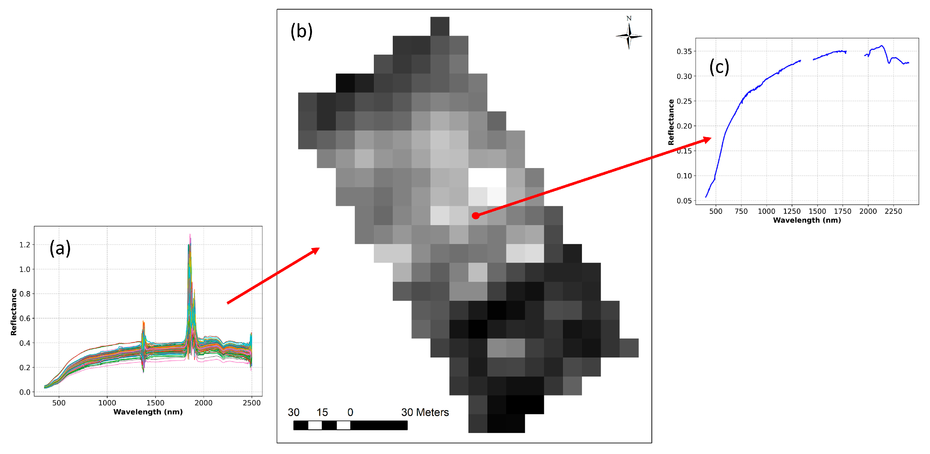
The spectral data consists of 2151 bands, which were pre-processed and reduced to 1693 bands after removing noisy bands. The raw spectra collected from 200 sampling points in the field are shown in Figure 3a.
The synthetic hyperspectral imagery with a 10 m pixel size, generated from 1693 bands through ordinary kriging, is shown in Figure 3b. A representative spectrum taken from a pixel is shown in Figure 3c. The kriging was carried out 1693 times for generating 1693 bands in order to construct a synthetic hyperspectral image of 10 m spatial resolution. Each time, the selection of semivariogram models was completed based on the lowest RMSE obtained from leave-one-out cross-validation. Exponential semivariograms, followed by spherical and Gaussian, gave the lowest RMSE compared with the others. The average RMSE values reported for exponential, spherical, and Gaussian semivariograms were 0.026, 0.030, and 0.030, respectively. The nugget, sill, and range parameters were estimated individually for each band while executing the kriging. For example, the ordinary kriging was carried out for band 10 using an exponential variogram model selected based on the lowest RMSE of 0.008 and MSE of 0.004. Here, the corresponding variogram parameters were a nugget of 0.000046, a major range of 0.0012, and a partial sill of 0.000079.

3.3. Model Evaluation and SOC Mapping

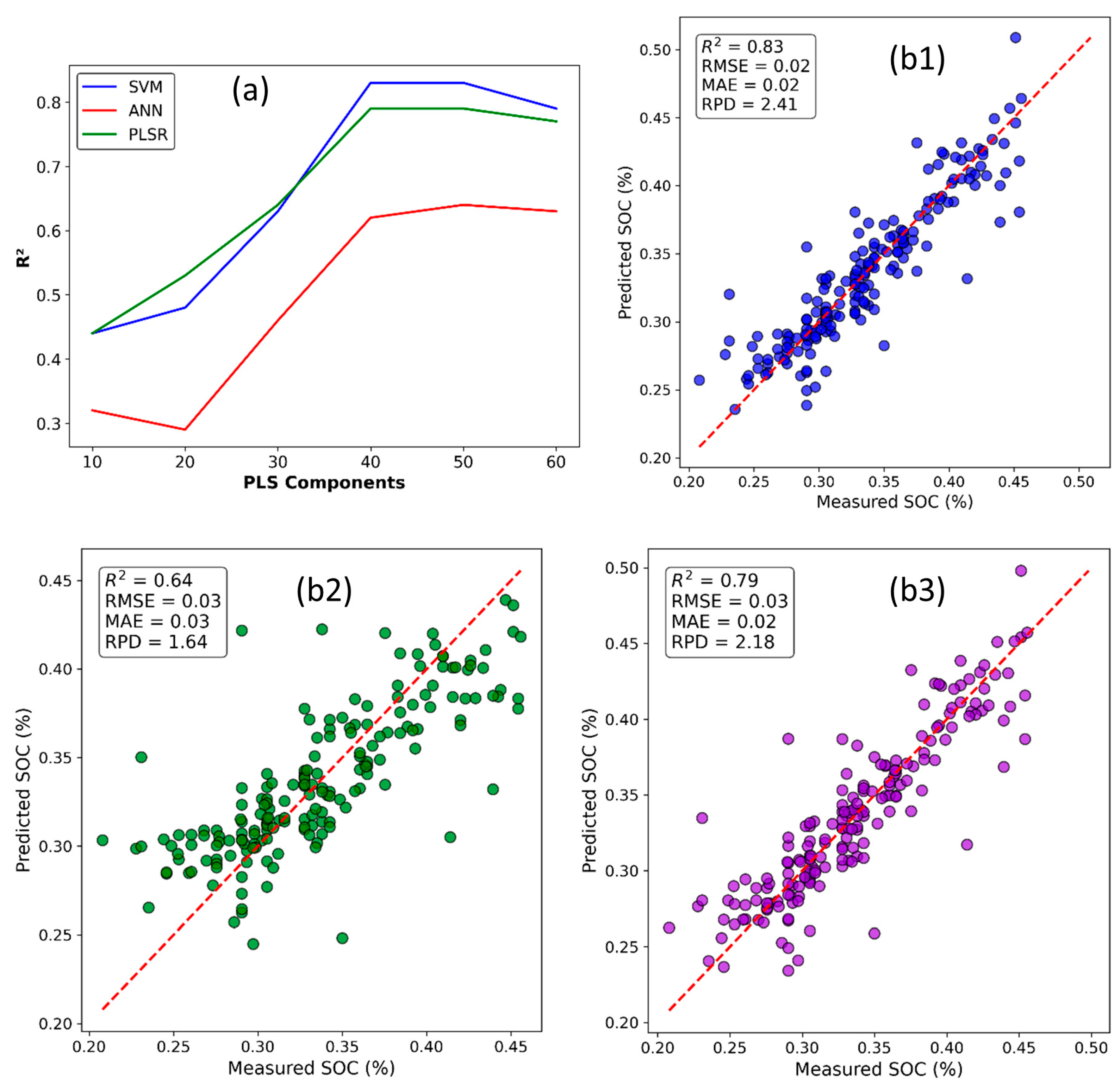
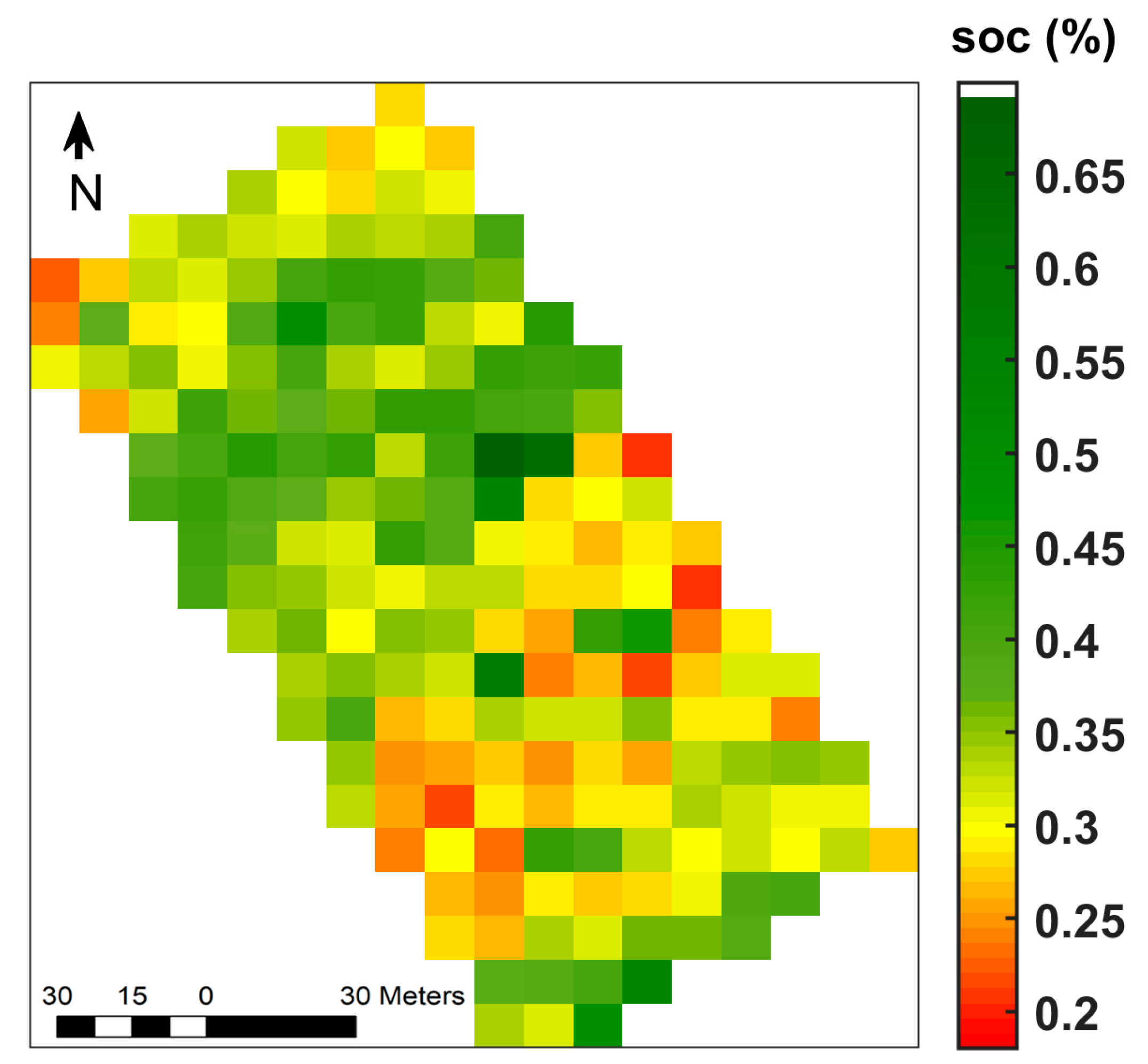
SOC prediction models of SVM, ANN, and PLSR were constructed using PLS components as the explanatory variables, and their accuracy was evaluated using five-fold cross-validation. The prediction accuracy was evaluated using multiple values of the number of PLS components to determine the optimal setting. The R2 shows an increase and becomes stable at 40 PLS components (as shown in Figure 4a), which was selected as the optimal number for prediction model development. The scatterplots of the predicted and measured SOC values, along with goodness-of-fit statistics, are shown in Figure 4b1–b3. The SVM shows the best fit and higher accuracy, with R2 = 0.83, RMSE = 0.02, MAE = 0.02, and RPD = 2.41, followed by PLSR and ANN. Through GridSearchCV, the optimal parameters chosen for SVM were kernel: linear, C: 0.1, and gamma: scale. For the ANN, the optimal parameters were batch size: 32, epochs: 200, learning rate: 0.005, and number of hidden layers: 4. The latent component count for PLSR was also set to 4. The best-performing SVM model was applied to synthetic imagery to generate a spatial map of SOC, as shown in Figure 5. The predicted SOC values exhibit variability across the field, indicating comparable results with the measured values.

4. Discussion

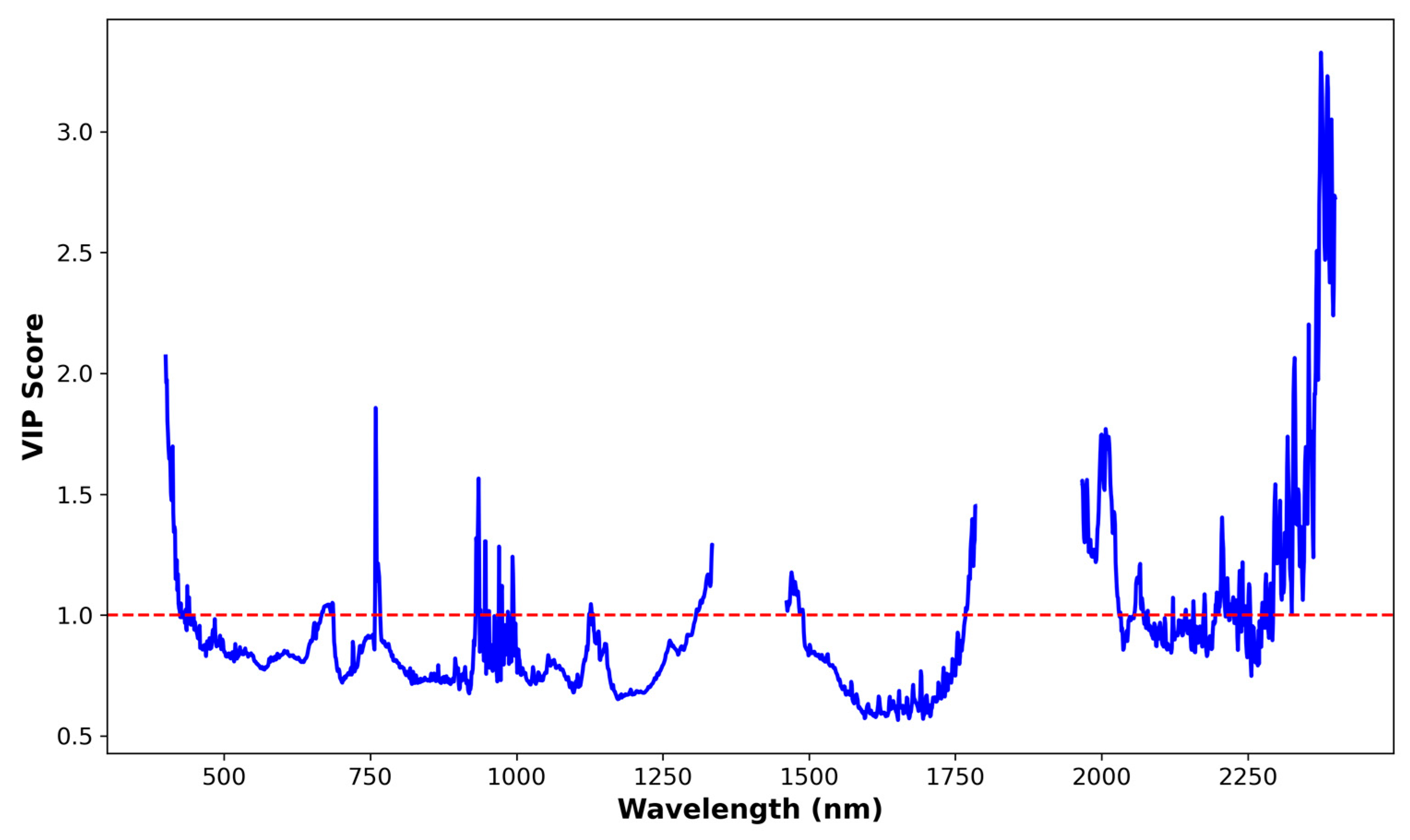
The superior performance shown by the optimized SVM model indicates an acceptable operational delivery of SOC maps at the field scale by using proximally collected spectral values. The outperformance of SVM in SOC prediction using hyperspectral data over other multivariate traditional models has been previously reported for hyperspectral data collected using proximal, airborne, and satellite spectroscopy [13,14,15,16]. The outperformance of SVM could be attributed to the model’s ability to manage the nonlinear relationships between SOC and spectral ranges [17]. Moreover, it was reported that, along with N, the carbon content can also be accurately predicted using spectral bands due to the presence of various overtones and blends of chemical bonds arising from carbon–carbon and carbon–hydrogen bonds [18,19]. A Variable Importance in Projection (VIP) plot (as shown in Figure 6) was generated to quantify the relative contribution of each wavelength across all 40 PLS latent variables calculated from the measured spectra. Wavelengths with VIP scores greater than 1 are considered the most influential for SOC prediction. The important bands obtained in the range of 400–900 nm are due to the presence of iron oxides (goethite, hematite), bands located around 1330 nm are associated with C-H bonds, around 2015 belong to C=O bonds, and more than 2200 nm are related to aliphatic C-H, C-O, C-N, etc. [20,21]. Most of the bands showing VIP scores > 1 closely coincide with previous findings [4,13].
The spatial variability of soil parameters depends on underlying materials, surface accumulations, and cultivation and input practices [13]. The present approach of generating synthetic hyperspectral data for soil OC mapping was tested on one field site with a limited number of samples, denoted by 16% of CV. A relevant follow-up study is needed to test this approach in multiple fields, covering larger sampling points to ensure transferability [21]. Beyond these three evaluated models, more machine learning models and deep learning frameworks, in combination with advanced feature selection techniques, can be considered in the future to attain higher accuracy [22]. As a continuation of the present work, synthetic imagery of mid-infrared spectral regions collected through Fourier Transform Infrared Spectroscopy will be employed in future for the more accurate prediction of soil fertility parameters [23]. At the same time, comparative studies with different imaging spectroscopic technologies, such as space and airborne hyperspectral missions, will also be considered in the future. Another critical point to consider is the application of a similar approach to other important soil fertility parameters, including micronutrients [24].

5. Conclusions

Synthetic hyperspectral imagery was generated using an ordinary kriging interpolation technique applied to non-imaging proximal spectroscopy collected from the field. Upon evaluating three machine learning models, the support vector machine demonstrated better accuracy (R2 value of 0.83) in predicting soil organic content. A high-resolution SOC map was also generated by applying the best prediction model to the synthetic imagery. The present work has opened up new research practices for the near-real-time delivery of accurate soil fertility maps using non-imaging spectral information.

Author Contributions

Conceptualization, R.G.R. and R.N.S.; methodology, R.G.R. and R.N.S.; software, R.G.R.; validation, R.G.R.; formal analysis, R.G.R. and T.K.; investigation, R.G.R. and R.R.; resources, T.K., A.B., R.R. and A.M.; data curation, R.G.R. and R.R.; writing—original draft preparation, R.G.R.; writing—review and editing, R.G.R. and R.N.S.; visualization, T.K., A.B., R.R. and A.M.; supervision, R.N.S.; project administration, R.N.S.; funding acquisition, R.N.S. All authors have read and agreed to the published version of the manuscript.

Funding

The results summarized in the manuscript were achieved as part of the research project “Network Program on Precision Agriculture (NePPA)”. This research was funded by the Indian Council of Agricultural Research (ICAR).

Institutional Review Board Statement

Not applicable.

Informed Consent Statement

Not applicable.

Data Availability Statement

The raw data supporting the conclusions of this article will be made available by the authors on request.

Conflicts of Interest

The authors declare no conflicts of interest.

References

  1. Wang, Y.; Huang, T.; Liu, J.; Lin, Z.; Li, S.; Wang, R.; Ge, Y. Soil PH Value, Organic Matter and Macronutrients Contents Prediction Using Optical Diffuse Reflectance Spectroscopy. Comput. Electron. Agric. 2015, 111, 69–77. [Google Scholar] [CrossRef]
  2. Jiang, R.; Sui, Y.; Zhang, X.; Lin, N.; Zheng, X.; Li, B.; Zhang, L.; Li, X.; Yu, H. Estimation of Soil Organic Carbon by Combining Hyperspectral and Radar Remote Sensing to Reduce Coupling Effects of Soil Surface Moisture and Roughness. Geoderma 2024, 444, 116874. [Google Scholar] [CrossRef]
  3. Padarian, J.; Minasny, B.; McBratney, A.B. Using Deep Learning to Predict Soil Properties from Regional Spectral Data. Geoderma Reg. 2019, 16, e00198. [Google Scholar] [CrossRef]
  4. Das, B.; Chakraborty, D.; Singh, V.K.; Das, D.; Sahoo, R.N.; Aggarwal, P.; Murgaokar, D.; Mondal, B.P. Partial Least Square Regression Based Machine Learning Models for Soil Organic Carbon Prediction Using Visible–near Infrared Spectroscopy. Geoderma Reg. 2023, 33, e00628. [Google Scholar] [CrossRef]
  5. Walkley, A.; Black, I.A. An Examination of the Degtjareff Method for Determining Soil Organic Matter, and a Proposed Modification of the Chromic Acid Titration Method. Soil Sci. 1934, 37, 29–38. [Google Scholar] [CrossRef]
  6. Pham, T.G.; Kappas, M.; Van Huynh, C.; Nguyen, L.H.K. Application of Ordinary Kriging and Regression Kriging Method for Soil Properties Mapping in Hilly Region of Central Vietnam. ISPRS Int. J. Geo-Inf. 2019, 8, 147. [Google Scholar] [CrossRef]
  7. Lu, P.; Niu, Z.; Li, L. Prediction of Soil Organic Carbon by Hyperspectral Remote Sensing Imagery. In Proceedings of the 2012 Third Global Congress on Intelligent Systems, Wuhan, China, 6–8 November 2012; IEEE: Orlando, FL, USA; pp. 291–293. [Google Scholar]
  8. Sahoo, R.N.; Rejith, R.G.; Gakhar, S.; Verrelst, J.; Ranjan, R.; Kondraju, T.; Meena, M.C.; Mukherjee, J.; Dass, A.; Kumar, S.; et al. Estimation of Wheat Biophysical Variables through UAV Hyperspectral Remote Sensing Using Machine Learning and Radiative Transfer Models. Comput. Electron. Agric. 2024, 221, 108942. [Google Scholar] [CrossRef]
  9. Sahoo, R.N.; Gakhar, S.; Rejith, R.G.; Ranjan, R.; Meena, M.C.; Dey, A.; Mukherjee, J.; Dhakar, R.; Arya, S.; Daas, A.; et al. Unmanned Aerial Vehicle (UAV)–Based Imaging Spectroscopy for Predicting Wheat Leaf Nitrogen. Photogramm. Eng. Remote Sens. 2023, 89, 107–116. [Google Scholar] [CrossRef]
  10. Rejith, R.G.; Sundararajan, M.; Gnanappazham, L.; Seenipandi, K.; Ramaswamy, S. GIS-Based Machine Learning Algorithms for Mapping Beach Placer Deposits in the Southwest Coast of India Using Landsat-8 OLI Images. J. Appl. Remote Sens. 2021, 16, 012011. [Google Scholar] [CrossRef]
  11. Das, B.; Manohara, K.K.; Mahajan, G.R.; Sahoo, R.N. Spectroscopy Based Novel Spectral Indices, PCA- and PLSR-Coupled Machine Learning Models for Salinity Stress Phenotyping of Rice. Spectrochim. Acta Part A Mol. Biomol. Spectrosc. 2020, 229, 117983. [Google Scholar] [CrossRef]
  12. Viscarra Rossel, R.A.; Walvoort, D.J.J.; McBratney, A.B.; Janik, L.J.; Skjemstad, J.O. Visible, near Infrared, Mid Infrared or Combined Diffuse Reflectance Spectroscopy for Simultaneous Assessment of Various Soil Properties. Geoderma 2006, 131, 59–75. [Google Scholar] [CrossRef]
  13. Mondal, B.P.; Sahoo, R.N.; Das, B.; Ahmed, N.; Bandyopadhyay, K.K.; Mukherjee, J.; Arora, A.; Moursy, A.R.A. Comparison of Multivariate Machine Learning Models for Major Soil Nutrients Prediction Using Laboratory-Based and Airborne (AVIRIS-NG) Visible near-Infrared Spectroscopy. Eur. J. Agron. 2025, 170, 127726. [Google Scholar] [CrossRef]
  14. Xu, S.; Wang, M.; Shi, X. Hyperspectral Imaging for High-Resolution Mapping of Soil Carbon Fractions in Intact Paddy Soil Profiles with Multivariate Techniques and Variable Selection. Geoderma 2020, 370, 114358. [Google Scholar] [CrossRef]
  15. Yang, J.; Dong, H.; Zhang, H.; Wang, J.; Dai, H.; Zhou, L.; Liang, T.; Zhang, Y. Enhancing the Estimation of Low-Spectral-Sensitivity Soil Properties: A Case Study of Active Organic Carbon Using Vis-NIR Hyperspectral Data. Int. J. Remote Sens. 2025, 46, 4941–4958. [Google Scholar] [CrossRef]
  16. Casa, R.; Pignatti, S.; Pascucci, S.; Castaldi, F.; Marrone, L. Estimation of Agronomic Soil Properties from Multitemporal PRISMA Satellite Imaging Spectroscopy. In Precision Agriculture ’23; Brill|Wageningen Academic: Leiden, The Netherlands, 2023; pp. 839–845. [Google Scholar]
  17. Gao, Y.; Cui, L.; Lei, B.; Zhai, Y.; Shi, T.; Wang, J.; Chen, Y.; He, H.; Wu, G. Estimating Soil Organic Carbon Content with Visible–Near-Infrared (Vis-NIR) Spectroscopy. Appl. Spectrosc. 2014, 68, 712–722. [Google Scholar] [CrossRef]
  18. Stenberg, B.; Viscarra Rossel, R.A.; Mouazen, A.M.; Wetterlind, J. Visible and Near Infrared Spectroscopy in Soil Science. Adv. Agron. 2010, 107, 163–215. [Google Scholar]
  19. Wenjun, J.; Zhou, S.; Jingyi, H.; Shuo, L. In Situ Measurement of Some Soil Properties in Paddy Soil Using Visible and Near-Infrared Spectroscopy. PLoS ONE 2014, 9, e105708. [Google Scholar] [CrossRef] [PubMed]
  20. Vasques, G.M.; Grunwald, S.; Sickman, J.O. Comparison of Multivariate Methods for Inferential Modeling of Soil Carbon Using Visible/near-Infrared Spectra. Geoderma 2008, 146, 14–25. [Google Scholar] [CrossRef]
  21. Xu, S.; Zhao, Y.; Wang, M.; Shi, X. Comparison of Multivariate Methods for Estimating Selected Soil Properties from Intact Soil Cores of Paddy Fields by Vis–NIR Spectroscopy. Geoderma 2018, 310, 29–43. [Google Scholar] [CrossRef]
  22. Odebiri, O.; Odindi, J.; Mutanga, O. Basic and Deep Learning Models in Remote Sensing of Soil Organic Carbon Estimation: A Brief Review. Int. J. Appl. Earth Obs. Geoinf. 2021, 102, 102389. [Google Scholar] [CrossRef]
  23. Engelmann, L.; Bierl, R.; Kirchhoff, M.; Ries, J.B. Application of Mid-Infrared Spectroscopy for Soil Analysis in Calcareous Argania Spinosa Forests in Morocco. Geoderma Reg. 2025, 42, e00964. [Google Scholar] [CrossRef]
  24. Mondal, B.P.; Sahoo, R.N.; Das, B.; Ahmed, N.; Bandyopadhyay, K.K.; Mukherjee, J.; Arora, A.; Ali Moursy, A.R. Digital Mapping of DTPA Extractable Micronutrients Using Combined AVIRIS-NG Hyperspectral and Multispectral Data of Sentinel-2 and SRTM-DEM. Comput. Electron. Agric. 2025, 239, 110905. [Google Scholar] [CrossRef]
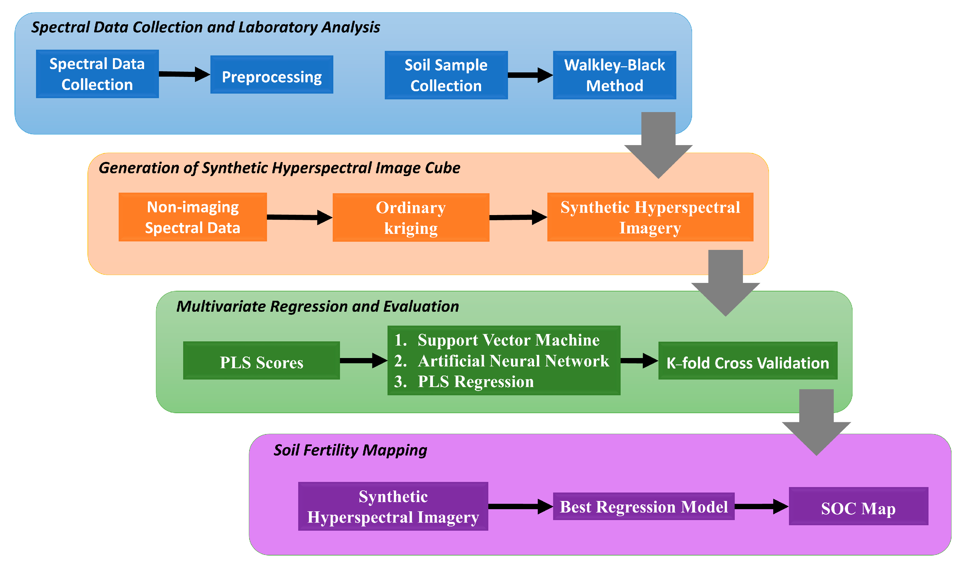
Figure 1. Flowchart of the methodology adopted for the present study.
Eesp 36 00003 g001
Figure 2. Study area map showing the spatial distribution of sampling points.
Eesp 36 00003 g002
Figure 3. Generation of synthetic imagery. (a) Raw spectra, (b) synthetic hyperspectral imagery (UTM Zone 43N, WGS84; pixel size: 10 m), (c) spectra correspond to a pixel.
Eesp 36 00003 g003
Figure 4. Performance evaluation of different prediction models. (a) Optimizing the PLS components, (b1) SVM, (b2) ANN, (b3) PLSR.
Eesp 36 00003 g004
Figure 5. Predicted SOC map generated by applying the SVM model to synthetic imagery (UTM Zone 43N, WGS84; pixel size: 10 m, SOC is expressed in %).
Eesp 36 00003 g005
Figure 6. VIP plots showing important spectral regions for SOC prediction. The red line denotes the threshold of 1.
Eesp 36 00003 g006
Table 1. Descriptive statistics of the measured SOC.
MinimumMaximumMeanMedianSD 1%CV 2 Skewness Kurtosis
0.180.520.330.330.0618.050.16−0.16
1 SD = standard deviation, 2 CV = coefficient of variation.
Disclaimer/Publisher’s Note: The statements, opinions and data contained in all publications are solely those of the individual author(s) and contributor(s) and not of MDPI and/or the editor(s). MDPI and/or the editor(s) disclaim responsibility for any injury to people or property resulting from any ideas, methods, instructions or products referred to in the content.