Simple Summary
Chacma baboons range in groups of 20–200 individuals across sub-Saharan Africa and travel as a group between resources such as food patches, sleep sites, and water sources. Although direct observation allows researchers to see when and why baboons stop, it is often difficult to observe every resource used on a daily basis, and it is almost impossible to know what resources the baboons did not use. Using retrospective GPS tracking data from collars placed on wild baboons, this study presents a method for identifying Areas of Interest (AOIs), some of which are known resources, and analyses how efficiently the baboons move between AOIs based on straight-line distance. We compare the routes the baboons took to the shortest-distance route, which should require prior planning, as well as a route that simply travels to the next closest AOI. We find that baboons take shorter routes than the nearest neighbour route but do not always take the most optimal route. This implies that baboons do plan their daily routes to an extent. These results provide insights into baboon cognition, as well as help identify how baboons choose where to go.
Abstract
The ability to navigate through both familiar and unfamiliar environments is of critical importance for foraging efficiency, safety, and energy budgeting in wild animals. For animals that remain in the same home range annually, such as grey-footed chacma baboons (Papio ursinus griseipes), movement efficiency is expected to reflect familiarity with the home range as well as the nature of the resources within it. For example, resources that are patchy, transient, or seasonal present a greater spatial cognitive challenge, and travel between them may be less efficient than for more widespread or permanent resources. Here, we analyse daily route efficiency in adult female grey-footed chacma baboons at Gorongosa National Park, Mozambique. We use GPS data taken at 15 min intervals from collars deployed on two baboons in each of two study troops (four total) to identify areas of interest used during daily ranging periods (sleep site to sleep site). We then compare the length of the route taken between a given day’s patches to routes calculated by two alternate optimisation heuristics as follows: the nearest neighbour method, in which the subject repeatedly travels to the next most proximate patch and does not necessarily return to the same place, and the Concorde algorithm, which calculates the shortest possible route connecting the day’s patches. We show that baboons travel more efficient routes than those yielded by the nearest-neighbour heuristic but less efficient routes than the Concorde method, implying some degree of route planning. We discuss our novel method of area of interest identification using only remote GPS data, as well as the implications of our findings for primate movement and cognition.
1. Introduction
Understanding how animals employ spatial memory, decision making, and planning during daily ranging activities is a key question in the field of movement ecology [1]. In wild primates, this question has been the subject of burgeoning scientific interest, particularly as technological advances increasingly allow researchers to overcome the challenges of accurately tracking these animals through complex landscapes [2]. However, the role of spatial cognition in shaping foraging paths is hampered by gaps in our understanding of how primates use past and present experiences to make movement decisions [3,4,5,6]. Multiple factors drive primate movement, including the distribution and profitability of foraging patches in terms of nutritional value per cost of search and travel (‘Optimal Foraging Theory’) [7,8,9], the cost of traversing the ‘Landscape of Fear’ [10,11,12,13,14], and other short-term considerations such as thermoregulatory factors including access to shade and water [15,16].
Various mechanisms have been identified that may help primates resolve the sometimes conflicting demands of these factors, such as the spatial and temporal mapping of risks and resources [13,17,18,19,20], episodic memory [21,22,23], and relying on knowledgeable leaders [24,25] or on the pooling of individual competences through collective decision making [26,27,28]. Quantifying the influence of these mechanisms allows researchers to better understand how primates make in-the-moment decisions, relying on information from the current state of the physical and/or social environment, and sometimes, prior experience. However, understanding how primates link sequential movement decisions over longer timeframes (e.g., over the course of a day of travel) and the extent to which they plan these decisions is a difficult task due to difficulties knowing not only where the primates travelled, but also where they chose not to go and what attributes influence their decisions [29].
Various studies have, nonetheless, sought to examine wild primates’ ability to plan and remember locations of interest (such as resource patches) and the paths that connect them, with apparent route planning being identified in several cases. De Guinea et al. (2019) measured landscape variables such as elevation and canopy density while observing wild black howler monkeys (Alouatta pigra), showing that the routes they used were located in areas of higher food-density than routes not used, implying they may have chosen those routes to monitor feeding trees [9]. A study on mantled howler monkeys (A. palliata) also found that they targeted mature fruits in long-distance movements [19]. Other arboreal monkeys, such as spider monkeys (Ateles belzebuth) and woolly monkeys (Lagothrix poeppigii), have also been shown to re-use routes to travel in areas with a high-density of food items [17].
In terrestrial primates, Noser and Byrne (2007) mapped out the most used resources of wild chacma baboons (Papio ursinus) and examined their ability to navigate between them when they were forced to detour from their normal routes. They found that the baboons made larger detours in areas with a conspicuous landmark such as a hill when compared with areas without prominent landmarks, implying that they navigate using a route network rather than Euclidean mapping [13]. Another study compared the movement patterns of humans and chimpanzees (Pan troglodytes) in a foraging context, using linearity and speed to measure spatial knowledge of the area and food locations, finding that while humans travelled at a constant speed but with higher linearity in familiar areas, chimpanzees decreased both speed and linearity in familiar areas [30]. This indicated that, while both species used spatial knowledge to navigate, chimpanzees appear to travel in a more ‘relaxed’ way in familiar areas, potentially due to an increased sense of safety, thus demonstrating that linearity and speed are not always suitable proxies for spatial knowledge, as found in other studies on chacma baboons [31]. A further study showed that, in areas with highly seasonal resources, home ranges and daily routes shift to preferentially utilise the available resources, representing a much larger shift in foraging strategy and route planning [32].
Despite extensive evidence that wild primates can establish, remember, and use travel routes, these routes and their networks may reflect the accumulation of past individual and collective experiences, rather than being the most optimal routes given the current state of the environment. Furthermore, studying the efficiency of travel paths in wild animals poses a challenge when the relevant destinations and/or intermediate stopping points are opaque to researchers. An oft-used method of testing travel efficiency is distilled in the Travelling Salesperson Problem (TSP). This long-standing optimisation problem invokes a travelling salesperson who must start at a given point, travel to a specific number of other points, and then return to the starting point by travelling the shortest cumulative distance; in studies of foraging animals, this translates to visits to multiple resources while minimising travel costs and thus maximising calorie gain [33]. Variations of this problem can be applied to animals that do not return to the same starting point at the end of the day; this variation is referred to as an Open-TSP, Hamiltonian Path Problem, or Shortest Path Problem [34]. In primates, whether or not an individual returns to the same sleep site repeatedly is often a product of habitat and sleep site availability rather than encoded at a species level, thus meaning that either the TSP or Open-TSP can often be applied to a single species [35].
One of the first studies of the TSP in captive primates was performed by Menzel (1973), where captive chimpanzees were able to optimise the route between food items hidden in their cages, thus obtaining them before their cage mates [36]. This method to test the efficiency of foraging and an animal’s ability to compute and plan multi-step routes has been studied in particular depth in bees (Bombus impatiens and B. terrestris). Using artificial setups of flowers over an observable area, it has been shown that given the opportunity, bees can learn the most efficient routes and maximise the distance to calorie trade-off [37,38]. Similar abilities to compute efficient routes between a set number of resources have also been found in pigeons (Columba livia) travelling between artificial goals [39]. Studies on captive vervet monkeys (Chlorocebus sabeus) were able to solve the TSP, although only with up to six locations in a 5 × 5 grid of feeding stations spaced 1.53 m apart [4].
Studies on wild vervet monkeys used an artificially established foraging patch to test route planning, showing that the vervets used relatively simple algorithmic processes, or heuristics, such as a cluster strategy or the convex hull, to solve the problem of connecting multiple resources, with variation in both individual foraging strategy and how often the shortest path was taken [34,40]. Without the use of artificial resources, it becomes considerably harder to measure route optimality, unless both a full resource distribution and the animals’ intended destination(s) are known in advance [41]. Nonetheless, several studies have successfully tackled the challenge of measuring route efficiency without using artificial resources. For example, wild tamarins (Saguinus mystax and S. fuscicollis), which travel on average only 2 km daily, were shown to be able to take efficient travel routes based on knowledge of the prior 1–21 days’ available resources more often than expected by chance [18]. In species that travel over larger distances, track linearity has also been used as a measure of route planning when all resources cannot be known. Valero and Byrne (2007) postulated that spider monkeys (Ateles geoffroyi yucatanensis) can plan multiple resources to visit in a single day, based on the assumption that linearity of travel reflected spatial memory [20]. It is worth noting that some studies [13,31] relied on handheld GPS devices carried by researchers during follows; thus, human influence on the recorded routes cannot be ruled out.
Although several of these studies claim to have found evidence that individuals were able to solve the TSP [18,34,39,40], a review by Janson (2014) showed that, in multiple studies, the distance travelled was no better than if the individual had used a relatively simple process, the nearest neighbour heuristic, in which the individual always travels to the resource most proximate to its current position and only the starting point determines the route rather than the overall layout of all points [29]. The limited space available for experiments in many captive studies means that there is little consequence to sequentially choosing the next nearest resource, whether or not this optimises the distance to return to the starting point from the final resource visited, thus making it difficult to decide how the route was chosen. However, in wild primates, where returning to sleep sites can add considerable cost to daily travel (and can be further constrained by predation risk and even conspecifics in cases of sleep-site competition), ensuring that the final resource visited is located near the sleeping site will be beneficial, even if it means not following the nearest neighbour heuristic. Unfortunately, the analysis of wild primate ranging data are often complicated by a lack of thorough knowledge regarding the distribution, location, and availability of resources in the environment, as well as the challenges of accurately tracking wild primates’ movement paths for the duration of entire days over an extended period.
Advances in biologging technology have improved our ability to tackle both the issues of knowing both where primates spend their time and how they reach those locations. GPS tracking devices attached to individual primates in the wild can be used to collect data on primate groups’ ranging patterns, their proximity to other groups; the speed, structure, and length of movement paths; and resource selection, such as the location of sleeping sites or foraging patches [28,42,43]. In this study, we introduce a novel technique of using GPS data to study foraging efficiency in wild chacma baboons (Papio ursinus griseipes) in Gorongosa National Park, Mozambique. We analyse GPS fixes taken at 15 min intervals from four individuals from two different troops over a total period of 332 days. Using cluster analysis to identify the most used areas in a primate’s day, hereafter referred to as Areas of Interest or AOIs, we remotely identify AOIs without the need for on-the-ground observations [44]. We quantify the efficiency of the route travelled between a given day’s AOIs and compare it with two hypothetical routes derived from (i) the nearest neighbour heuristic and (ii) the optimal (least distance) route. By calculating the difference in distance travelled between the actual and the two hypothetical routes, we evaluate how efficiently baboons move between AOIs in their own environments and the ways we can use current and historic GPS data to answer questions about primate movement, even in the absence of direct observational data.
2. Materials and Methods
2.1. Study Site and Subjects
Data were collected from four GPS-collared grey-footed chacma baboons (Papio ursinus griseipes) from two different troops in Gorongosa National Park (GNP), Mozambique [45,46]. GNP consists of a heterogeneous, mosaic landscape, with distinct dry (April-October) and rainy (November-March) seasons [47]. Although the Mozambique Civil War decimated the mammalian wildlife of GNP, the Gorongosa Restoration Project has managed to largely recover much of the herbivore population, as well as an increasing number of lions, crocodiles, and a high density of baboons [48,49,50]. Additionally, during the study period, two packs of wild dogs were introduced into GNP, although no resident leopards, a main predator of baboons, were known to range within GNP. Two cycling, adult female baboons with no dependent offspring were collared from each of two study troops, the Floodplain (FT) and Woodland (WT) troops, which have been followed on foot and studied periodically since 2017 as part of the Paleo-Primate Project Gorongosa. The collared monkeys were named Acacia (Woodland), Kigalia (Woodland), Eve (Floodplain), and Abacaxi (Floodplain). The systematic habituation to observers of the Woodland troop began in July 2017 and that of the Floodplain troop in May 2018. Adult females were chosen to ensure the collared individuals would not disperse over the course of the study; two individuals were chosen per group to make sure the troop could still be tracked in the event one collar failed.
Prior to a pilot season in 2017, the baboons of GNP had not been systematically studied, and WT was only periodically observed after September 2019. Consistent study on FT was further hampered by the COVID-19 pandemic. Additionally, a major cyclone devastated the area in early 2019, during which the majority of juveniles in FT disappeared [51]. Therefore, individual relationships, social hierarchies, and reproductive cycles of both troops are as yet unevaluated. However, observations show that the baboons engage in daily routines and behaviours similar to other field sites, with subgrouping occurring throughout the day.
FT (n = approx. 30 individuals) ranges on the floodplain in the southern-central portion of GNP, covering around 15 km2 based on the minimum convex hull of 95% of their ranging points. This area consists primarily of alluvial floodplain with some fever tree (Vachellia xanthophloea) woodland. Their ranging area is bordered by the Tsungue River to the east and bisected by the Mussicadzi River to the west and south. These rivers are seasonal and during most points of the year can be crossed via wading, jumping, fallen trees, or sand banks, except during seasonal floods. FT’s diet consists primarily of sedges, Vachellia seed pods, and some palm fruits, with opportunistic hunting of small birds, shellfish, and mammals [52].
WT (n = approx. 90 individuals) ranges in approximately 7.5 km2 in the woodlands directly south of the Floodplain troop’s home range. This area is primarily made up of medium-to-dense Vachellia–Combretum woodland, interspersed with seasonal water pans and termite mounds. WT’s diet consists mostly of leaves and fruits, with opportunistic hunting of small mammals [53]. The extreme north of the WT’s home range is bordered by the Mussicadzi River.
FT’s relatively larger home range can be explained by the seasonal flooding of GNP. From November to April, annual rains inundate the central area of GNP, forcing wildlife towards the edges into a virtually new home range [54,55]. During the dry season, FT utilise the northern half of their range, and they migrate to the southern portion during the wet season. For further information on the study subjects and satellite imagery, vegetation, and the distribution of water resources in each home range, see Lewis-Bevan (2024) [52] and Supplementary Figure S1.
2.2. Data Collection
The four baboons were darted and collared between late July and mid-August 2019. Each baboon was fitted with a GPS/accelerometer collar (model 1D, e-obs Digital Telemetry, Grünwald, Germany) by an experienced vet following anesthetization using ketamine (15 mg/kg) via dart gun. Individuals were chosen opportunistically, as long as they met the criteria of being an adult female with no dependent offspring. Each collar was programmed to record a burst of 10 GPS points every 15 min UTC time, at the minute intervals of :00, :15, :30, and :45. Collars collected data until the end of their battery life, which varied for each collar, ranging from 293 to 323 days. GPS data were downloaded from the collars monthly from August 2019 to November 2019, then again in February 2020, May 2020, and June 2020, using an eObs BaseStation II connected to a Yagiantenna (868 MHz 10E) at a distance of 10–50 m (e-obs Digital Telemetry, Grünwald, Germany). Each data download was continued until registered as complete and contained successful fixes since the last download. Downloaded data were then processed using Eobs decoder_v10s1.
2.3. GPS Data Processing: Daily AOIs and Routes
For the purposes of our analysis, from each burst of GPS fixes at 15 min intervals, only the last GPS fix in each burst was used. GPS records were split into discrete calendar days for analysis, containing the GPS points for that day including and between sleep sites, but discarding overnight GPS points. Within each GPS day, these GPS points were divided into ‘waypoints’, or areas where the baboons spent substantial time (>15 min; see below for more detail). Because baboons are diurnal, the first and last waypoint of each day was automatically the sleep site, determined as the GPS location at 0200 h UTC on the study day (“morning sleep site”) and 0200 h UTC on the next day (“evening sleep site”). When the collars failed to detect satellites at 0200 h, 0230 h was used. Because the baboons did not always sleep at the same place on consecutive nights, the problem being solved often became one of an Open-TSP, wherein an individual is not required to return to the same starting point to end, although hereafter we refer to the problem being solved collectively as TSP for simplicity.
Once sleep sites were identified, GPS data were first filtered only for points that were taken a minimum of 50 m from either the morning or evening sleep site. This was to ensure that only the sleep site was considered a waypoint for that area and not any areas used for basking or waiting for the rest of the group to emerge from the sleeping tree.
Through previous daily follows of the baboons, areas were observed where the troops tended to forage or spend time napping or socialising (LLB, personal obs.). Areas where baboons spent a significant amount of time were therefore considered to be AOIs, often containing a resource for either foraging, resting, sheltering, or socialising. To identify AOIs without observational data, the filtered GPS points were ordered sequentially by date and time. The first GPS point was considered the “anchor” point. The distance between each subsequent GPS point and this anchor point was compared. If the subsequent GPS point fell within 30 m of the anchor point, which was roughly the spread of FT during a foraging bout (LLB, personal obs.), it was considered part of the same group of points (GoP). If a GPS point fell outside of the 30 m radius, it became the anchor point of a new GoP. If there were no GPS points within the radius of a point, that point became its own GoP. This method was repeated sequentially through all points until no GPS points were left.
The created GoPs were then filtered to only include groups with two or more GPS points, as this signified that the monkey had remained in that area for at least 15 min. GoPs were then clustered using the hclust function from the R package ‘stats’ [56], where any GoPs in the same month that fell within 40 m of another GoP were combined to form a new waypoint cluster, or a polygon [44]. This was to increase the likelihood that waypoints indeed indicated an AOI, i.e., the presence of something that could be exploited in that area multiple times, rather than the area acting as a one-off stopping point for hunting, predation avoidance, or other non-repeatable reasons. This aggregation also meant that AOIs which were in very large, continuous, depletable patches, such as areas with seasonal sedges or clusters of palm trees, would be counted as a single AOI rather than multiple small ones. The geometric centre of each of these clusters was used as the defining GPS point for a waypoint.
To calculate daily routes between waypoints, each daily GPS track (generally 96 points/day per monkey) was compared to the waypoints of that month, and it was noted whether each GPS point, in turn, fell within the polygon of a waypoint. Waypoints were discarded if only one GPS point fell within a polygon, as this indicated the baboons had passed but not stopped to utilise the AOI. The order of the final waypoints as they appeared in the daily GPS tracks was the order of waypoints for that day, regardless of points that did not fall within a polygon, and this was defined as the day’s route.
A day’s route was defined as usable for analysis if the monkey had (a) visited more than two waypoints while travelling between sleep sites and (b) did not revisit any waypoint. This was to ensure that calculating an optimal route was neither trivial (in the case of too few waypoints) nor too complex (if allowing for revisits to waypoints on the same day). In identifying days that matched the criteria for usability, we found that around or just over half the days of each monkey were unusable for this type of analysis, mostly due to revisits to waypoints.
2.4. Comparison of Actual Travel Routes to Nearest Neighbour and Branch-And-Cut (Concorde) Route Optimisation
All analysis was carried out using RStudio Version 1.3.95946 [57]. Once a daily route between waypoints was discerned from the GPS points, two types of route optimisation were used as comparison, the “Nearest Neighbour” (NN) and “Branch-and-Cut” (Concorde) methods. The NN method is considered a “greedy” but easy method. Each sequential node is chosen based on proximity to the previous one, using only local information, without long-term planning regarding the location of the start or end point of the route (i.e., the morning and evening sleep sites, respectively) [29]. This allows for short travel distances between consecutive waypoints, but it can lead to long travel distances between the penultimate node and the final node when individuals must return to the starting point.
The Concorde method is so named because it relies on the Concorde TSP solver [58] to select the most optimal route based on all possible routes, with the most optimal route being the one which requires the least distance travelled to cover all nodes and still return to the starting node. The comparison of all possible route distances was performed using the R packages sp [59,60] and tspmeta [61]. In the former, the function spDists() calculated distance matrices between each pair of waypoints, including sleep sites, in a day. These distances were calculated in Mercator projection (UTM), for precision across short distances, and were taken to be the beeline distance, without accounting for physical barriers or elevation changes (such changes were in any case negligible; the main barrier in the home range of either troop was the Mussicadzi river, which WT never attempted to cross and FT crossed with little diversion via sandbanks, fallen trees, wading, or jumping from tree crowns to the opposite bank). The latter package was used to determine the NN and Concorde routes for each day, using the same distance matrix each time.
Due to the constraints of the Concorde solver and its inability to solve Open-TSPs, it was necessary to manipulate the data such that the routes started and ended at designated points, specifically the morning and evening sleep sites. To accomplish this, within the distance matrix, distances to and from sleep sites were manipulated while maintaining the symmetry of the distance matrix. The distance between the first point—the morning sleep site—and the last point—the evening sleep site—was set to have a negligible cost, at 0.000001 m apart. However, the distance between the morning sleep site and all other points besides the evening sleep site was set to have extreme cost, by adding 10 km to the total distance. This ensured that there would always be a high cost to returning to the morning sleep site, thus making it most optimal to start there, and the model started and ended with each sleep site. For the NN analysis, because the chosen path depends on the start point, the start point was set as the evening sleep site. This forced the model to then choose to go to the morning sleep site and to pick the NN route from that point, before returning to the evening sleep site. Once the routes were created, the sequence of points was reordered to start with the morning sleep site and end with the evening sleep site, simply shifting the start and end of the sequence (e.g., when the model produced the order “End-5-2-3-Start”, this was translated to “Start-3-2-5-End” for analysis, with Start being the morning sleep site and End being the evening sleep site).
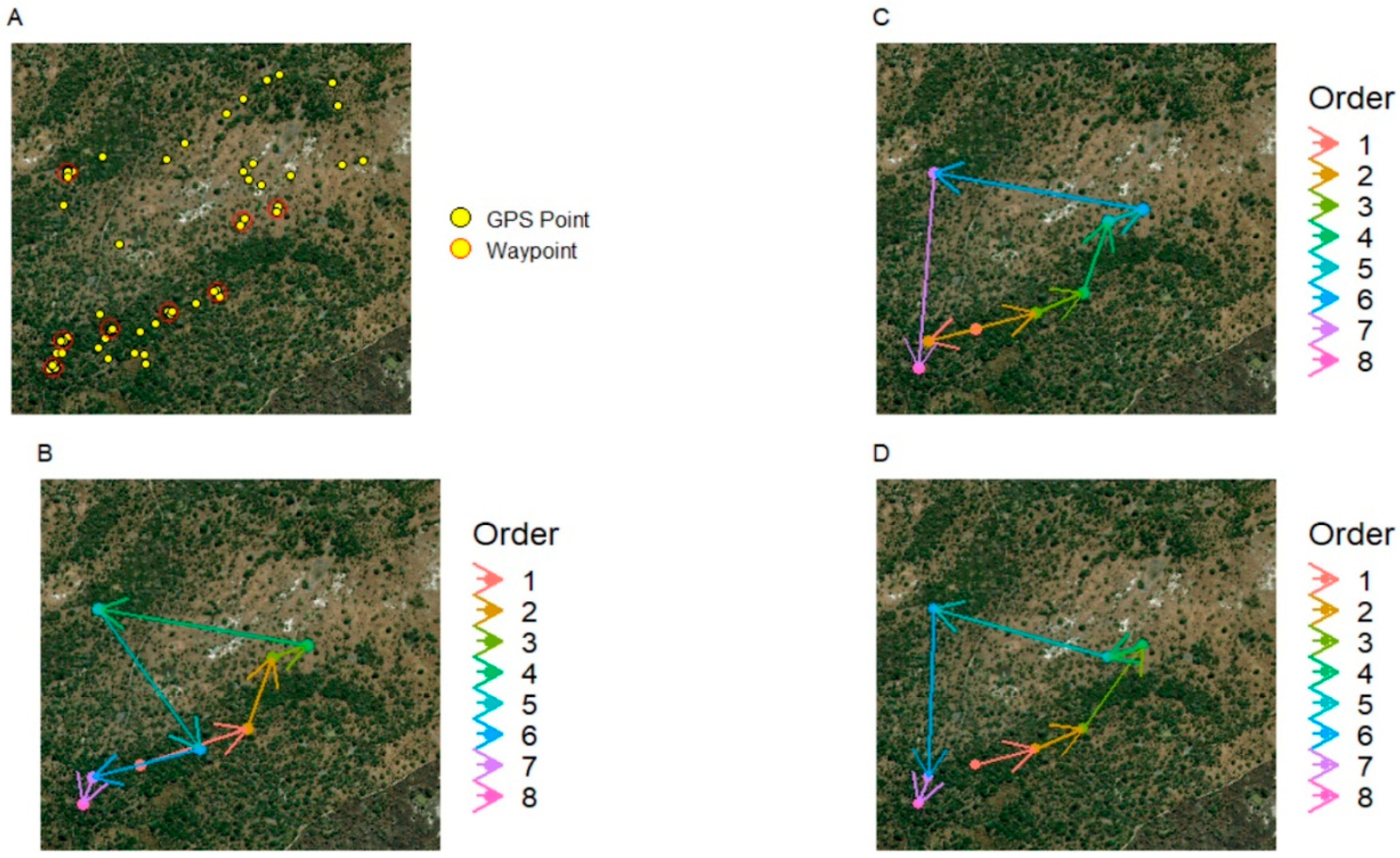
Once the Concorde and NN routes were determined, the cumulative distance of each day’s modelled routes was compared to the actual route for that day, as described in the following section (see also Figure 1 for an illustrative example of a single day’s actual, NN, and Concorde routes).
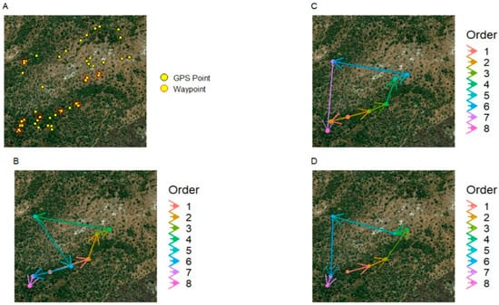
Figure 1.
A single day’s tracks taken from the Woodland Troop. (A) Yellow dots show GPS fixes recorded for the day; red circles indicate clusters of points that were identified as waypoints. (B) The actual order in which the troop travelled between the waypoints identified in (A). (C) The hypothetical route calculated by the Nearest Neighbour heuristic for the same set of waypoints. (D) The hypothetical, maximally efficient route calculated by the Concorde optimiser.
3. Results
Across the four GPS-collared monkeys, 714 travel days were available for analysis once unusable days had been discarded (Table 1). Note, however, that these figures underestimate the real distances travelled since the distances between consecutive GPS fixes are calculated as straight-line distances. Collars failed to acquire, or failed to download, preprogrammed fixes <1% of the time for all monkeys except Acacia (WT), whose collar failed to acquire fixes or acquired an impossible fix around 4% of the time. For all monkeys except Acacia, horizontal accuracy was measured as roughly 5 m ± 5 m; for Acacia, accuracy was measured at 10 m ± 8 m.

Table 1.
Summary data of individual monkeys’ daily statistics for analysed days. Min and Max waypoints indicate the minimum and maximum waypoints each monkey visited in a day. Days matching Concorde indicates how many days analysed the monkeys travelled on the same route as the Concorde solver and the minimum and maximum waypoints on those days.
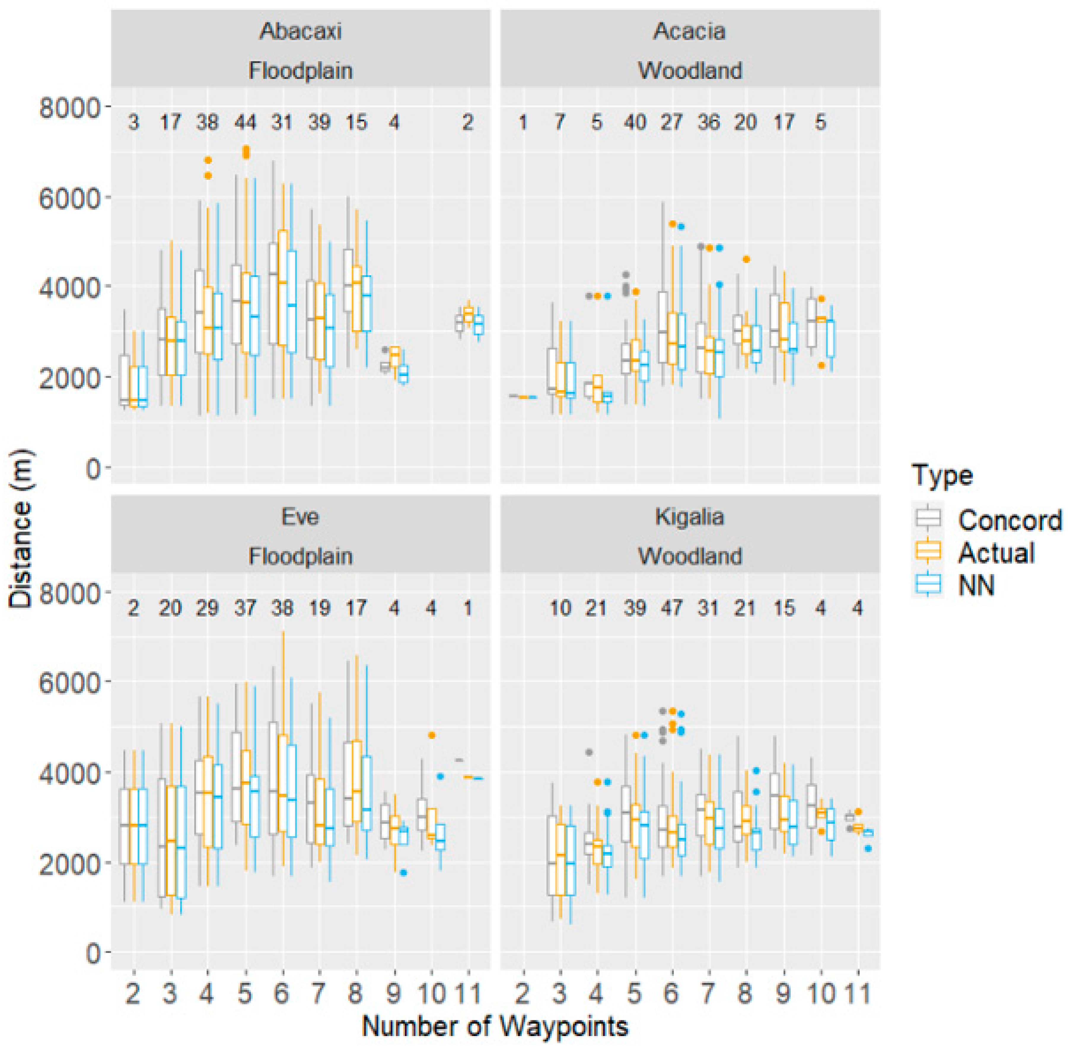
Comparisons of daily route lengths calculated for the actual, NN, and Concorde routes are shown in Figure 2 and Figure 3. A paired, two-sided Wilcoxon Signed-Rank Test for each monkey showed significant evidence that, for all monkeys except Abacaxi, there is a difference between the length of the NN route and the actual route length taken.
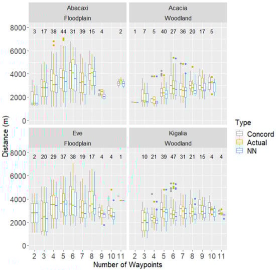
Figure 2.
Comparison between actual daily travel paths recorded from wild baboons and hypothetical paths derived from two different path optimisation procedures (NN and Concorde) connecting daily waypoints. Distance travelled per day shown as a function of the number of waypoints visited that day. The numbers above each box indicate how many days with the number of waypoints on the x-axis were analysed for each monkey.
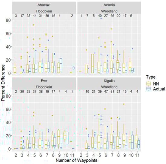
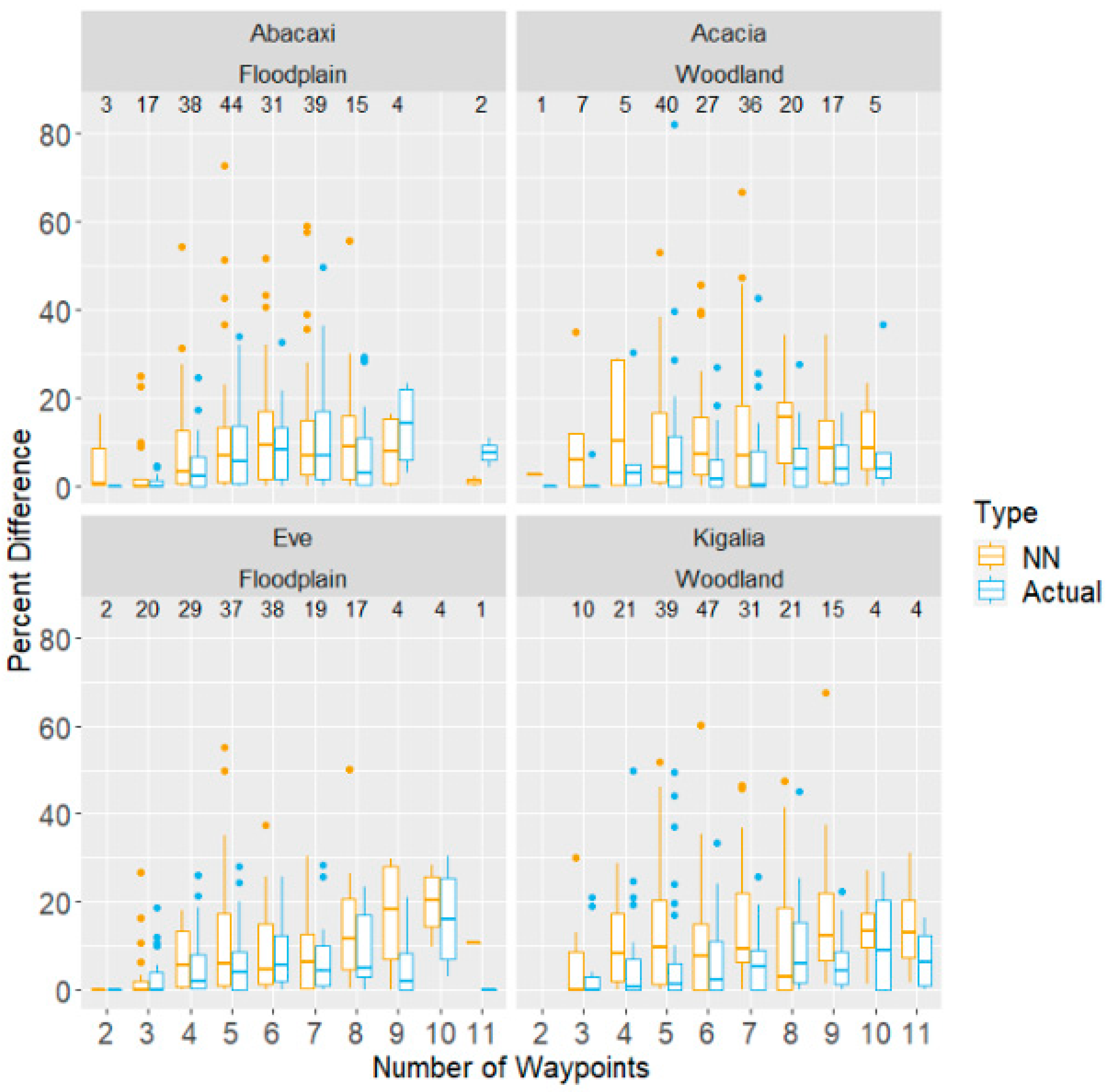
Figure 3.
Additional distance travelled, expressed as a percentage of that day’s optimal (Concorde) distance, for both NN and actual route distance, as a function of the number of waypoints visited that day. Each panel corresponds to data from one of the four subjects, with troop also labelled. Boxplots show quartiles and range, with points plotted individually if they are above or below the lower quartile by at least 1.5 times the interquartile range. The number of days with each number of waypoints is shown above the boxplots.
Further analysis using a paired, two-sided Wilcoxon Signed-Rank Test showed evidence that, for all monkeys, the actual route taken was more likely to be shorter than the NN route. By contrast, a paired, one-sided Wilcoxon Signed-Rank Test showed evidence that all monkeys’ routes were longer than the Concorde route of each day. The results of these tests can be found in Table 2.
Table 2.
Summary of paired, one-sided Wilcoxon Signed-Rank Tests comparing the lengths of route types. Column one shows that the length of the nearest neighbour route is significantly different from the length of the actual route for all monkeys except Abacaxi. Column two shows that for all monkeys, the actual route was statistically longer than the Concorde route, while column three shows that the actual route was statistically shorter than the nearest neighbour route.
In examining how inefficient the baboons’ routes were, the number of waypoints emerged as a significant predictor of inefficiency, where relative to an average route of five waypoints, each additional waypoint increased inefficiency by about 0.82 percentage points (DF = 709, F-stat = 8.74, p < 0.01; see Figure 3). However, each monkey matched the Concorde route multiple times on days with routes ranging from 2 to 11 waypoints. The highest number of waypoints matched varied by monkey; Kigalia matched the Concorde solver on one day with 11 waypoints, while Acacia was able to match it on a day with 10 waypoints, Eve on a day with 9, and Abacaxi on a day with 8.
4. Discussion
Close to half a century ago, Altmann (1974) emphasised that a primate’s movement decisions should be expected to be based, in part, on obtaining the most calories for the least distance travelled, leading to further research inspired by optimal foraging theory and foraging efficiency [33,62]. Therefore, understanding how well primates solve the TSP daily—that is, how they set out from their sleep site in the early morning; travel to enough resources throughout the day to fulfil needs for food, water, shelter, and sociality; and then return to the same (or different) sleep site in the evening while being as energetically efficient as possible—is key to understanding primate memory, decision making, and spatial planning.
The TSP has been used in previous studies with mixed results, with claims of individuals of some species succeeding at finding the most efficient route, while others have not [4,29]. Previous studies on baboon route planning showed that baboons were able to use some (albeit limited) level of multi-step route planning, based on observational and experimental data [13,31]. In this study, we made use of a different technique to build on these findings as follows: we used remotely collected data, applied to an often Open-TSP, to develop a new method of measuring route efficiency using location data taken from GPS-collared chacma baboons. By clustering points into areas where the study subjects remained for at least 15 min, we were able to identify areas of interest to the monkeys, which we have called “waypoints” (the likely location of resources such as food, shade, or shelter). The number of these waypoints each group visited in a day varied between 2 and 11 over the course of 332 days of data collection, although the two collared monkeys in each group did not necessarily both visit each waypoint identified for a given day. We then compared the monkeys’ daily routes connecting these waypoints with hypothetical routes computed using the following two different algorithms: the NN heuristic and the Concorde optimiser.
Our results show that the baboons performed better than the NN model, but worse than the Concorde optimal model. The NN heuristic is a simple but greedy heuristic, wherein it seeks to travel between waypoints as quickly as possible without regard for the efficiency of the overall route. Performing better than this model implies that the baboons did not simply choose always to travel to the next nearest AOI from their current one, but they were instead able to sacrifice some immediate gain for benefits later in the day (i.e., they may have travelled past possible AOIs to a distant AOI and then returned to stop at them on their approach to a sleeping site). This is seen in the data, particularly on days where the NN distance travelled was more than a kilometre longer than the actual route (n = 27 days), and in one case the difference was as much as 3 km. This may imply some degree of planning, given that the baboons were able to travel between a given set of waypoints in a more efficient manner than by repeatedly moving to the next nearest waypoint.
On the other hand, the baboons performed significantly worse than the Concorde model, which is to be expected given the computational demands of calculating the optimal route. However, on 218 days across all four monkeys, the baboons were able to find the most efficient route with days ranging from 2 to 11 waypoints (Table 1). While it is expected for subjects to find the optimal route by chance on days with fewer waypoints, their ability to find the optimal route on days with a greater number of waypoints makes a much stronger case for the involvement of planning. Indeed, while we found that overall route efficiency decreased as the number of waypoints increased (which is not surprising given that the difficulty of the task increases greatly with the addition of extra waypoints), the baboons were able to find the optimal route at least once on a day with 11 waypoints and used the optimal (i.e., Concorde) route on about 20% of days with 4–10 waypoints. Nonetheless, there are several explanations we can propose to account for the observation that on the majority of days the baboons’ routes were suboptimal.
First, the baboons may be constrained by their own abilities to map space and/or to plan. One study found that baboons may not be able to form Euclidean map-like representations [13], which makes the task of finding the shortest route between points more difficult. However, another study suggested that baboons may use episodic memory and a cognitive map to plan their routes in advance [31]. Second, since baboons travel in groups, any movement that an individual performs will result from a combination of their personal preference and those of the others in the troop. As such, the group consensus is likely to be a compromise between multiple individuals’ preferences, meaning that even a hypothetical perfect route optimiser may need to compromise on the route travelled [28]. The effect of group decision making is compounded in the baboons studied here, as their group spread is often hundreds of metres, potentially allowing them to exploit multiple AOIs at the same time. Third, because AOIs are heterogeneous in nature (food, shade, etc.), the order of waypoints may not be as random or free as it is in the case of the NN and Concorde algorithm. For example, baboons may pass a shady patch without stopping in the early, cooler part of the day, only to return there later when temperatures soar, leading to what appears to be a suboptimal path purely from the perspective of path length. Fourth, and perhaps most crucially, we cannot be sure how many of a day’s waypoints are ‘fixed’ at the beginning of the day, and hence, how many waypoints ahead we can expect baboons to plan.
Besides these theoretical considerations, our results are also complicated by the nature of our data. We used remotely collected data—a method of studying primate, or indeed any animal, movement without the need for on-the-ground observation of the subjects. Thus, we also established a novel method for identifying locations of interest (‘waypoints’), but this technique has several limitations. In particular, the time-based definition of a waypoint means that some “false” waypoints may have been identified. Pauses presumed to be for a stationary AOI could have come about from an opportunistic hunt, an unexpected intergroup or predator encounter, a weather phenomenon such as rain or extreme heat, or even a newly discovered AOI that the troop happened upon. Without knowing the exact nature of each identified waypoint, it is difficult to fully evaluate the subjects’ capacity for route planning. However, stricter definitions of what constitutes a waypoint, the integration of on-the-ground surveys, geographical and vegetation data, conspecific ranging data, and historical weather data could all help to clarify waypoints used in each model. Conversely, it is possible that our criteria for a waypoint are too restrictive and that the monkeys are in fact visiting additional waypoints undetected by our analysis (which would render our comparisons with the calculated hypothetical routes less informative). Again, additional environmental data, as well as adjusting the parameters for what constitutes a waypoint for each study site, would help to minimise this issue.
Although the baboons observed in this study were seen to return to the same areas over multiple days to forage, it should also be noted that the patches varied in size and shape, particularly for FT, who tended to forage on patches of sedges rather than distinct trees [52,53]. Parameters for a patch or waypoint were chosen based on the average observed size of food resources, including tree crowns. However, ground patches of food were more variable. As sections of the patch were depleted or became ready for consumption, the overall shape and, in some cases, location of the patch changed. The current method of identifying waypoints may be too coarse to account for these discrepancies. Weekly patch monitoring, either in person or using remote sensing, could help inform the best parameters of waypoint identification over time.
An additional limitation of our method is the uncertainty of how the primates chose these waypoints. Studies have shown that group movements in baboons, even when initiated by a single leader, are “voted upon” democratically [26,28,63]. While we interpret our results assuming that the baboons aimed to visit the patches we identified as waypoints, we cannot exclude the possibility that they opportunistically found patches over the course of their daily ranging or simply picked a patch and then continued on to each subsequent patch as it was remembered or “voted upon” by the group. Nonetheless, our results show that this is unlikely, given the greater efficiency of the baboons’ routes compared to those produced by the NN algorithm. Further, because the full social hierarchies, or even demographics, of each group were unknown, it is impossible to say whether certain individuals influenced the group’s movement decisions more than others or even constrained some individuals from entering foraging patches; future studies should consider more selectively collaring known “leaders” and “followers” within the study group to compare the routes taken by each.
Another consideration of the study’s limitations concerns the nature of the study site. At the time of the study, the density of predators in GNP was relatively low, and the number of resident leopards, the main predator of baboons, was presumed to be zero (although leopards were occasionally spotted transiting through GNP on camera traps) [49]. Therefore, there may have been less pressure on the baboons to find optimal routes, given they were less constrained by the threat of predation and the need to find a suitable sleeping site by dusk. The lack of predators may have also led to an increase in baboon density in GNP, with aerial counts showing 225 troops in the central 1845 km2 of the park [50]. Additionally, troops were often seen to overlap home ranges, suggesting the avoidance of inter-troop encounters may have been prioritised over minimising daily travel distance (LLB, personal observation). The high density of troops may lead to a prioritisation by the baboons to travel more quickly to exhaustible resources, such as fruit trees, and return to more homogenous patches later in the day. However, in April 2021, leopards were reintroduced to GNP, and a comparative analysis of similar data should be undertaken to understand the effects of increased predation on route planning and actual routes travelled.
Besides predation, the extreme seasonality of GNP was also not explored in this study, due to the majority of analysed data being collected in the wet season. This could be due to more unusable days (i.e., days where monkeys return to the same waypoint after visiting it the same day) occurring during the dry season. However, the visual inspection of the distribution of the number of daily waypoints shows an emerging seasonal pattern. While the Woodland Troop exhibits no apparent change in the number of daily waypoints across seasons, the Floodplain Troop increases the number of daily waypoints in the wet season and decreases them in the dry season. The change in waypoints also, naturally, leads to the opposite change in efficiency, with days with more waypoints associated with lower efficiency and days with fewer waypoints associated with greater efficiency. This change in the number of waypoints in the Floodplain Troop may be the result of greater resource abundance in the wet season compared to the dry, physical barriers such as floodwater, or the seasonal change in home range size or physical shift in home range, with larger home ranges potentially being an artefact of fewer available resources [64,65]. Further analysis, combined with future studies including on-the-ground data, may reveal more seasonal effects on route optimality in these baboons.
In sum, we aimed to study primate cognition through natural movement using only remote data, and, in the process, we established a new method of studying spatial decision making without the need for observational data. Our results provided evidence that baboons may be capable of some degree of planning of their daily travel routes, producing routes that are more efficient than a simple heuristic of iteratively moving to the next nearest location of interest. While these results come with caveats, they demonstrate a novel approach to examining primate decision making in the context of daily travel using remotely collected GPS data. This method can be further refined to include alternate remote sensing data, create more robust results, and offer a new and practical way to utilise previously collected data or future data sets. The use and refinement of this method paves the way for further cognitive studies using historical GPS data across a variety of species and allows researchers to utilise their data sets for multiple purposes beyond the originally intended study.
5. Conclusions
We identified areas where baboons repeatedly spent more than 15 min over multiple days, or Areas of Interest (AOIs), using spatial clustering of GPS fixes. When travelling between them on a daily path, the baboons of GNP were able to travel more efficiently than predicted by the Nearest Neighbour heuristic, but they were not always able to take the most optimal route. We show evidence of route planning in the baboons’ daily movement. Refinement and further development of using clustering to identify AOIs could allow for more in-depth analysis of GPS data without the associated covariates.
Supplementary Materials
The following supporting information can be downloaded at: https://www.mdpi.com/article/10.3390/wild2020018/s1, Figure S1: A comparison of satellite imagery and habitat classification of the baboons’ main ranging areas.
Author Contributions
The contributions of each author are as follows: Conceptualization: L.L.-B. and D.B.; Methodology: All Authors; Software: L.L.-B.; Validation: L.L.-B.; Investigation: L.L.-B. and P.H.; Project Administration: All Authors; Resources: All Authors; Formal Analysis: L.L.-B.; Visualisation: L.L.-B.; Writing—original draft: L.L.-B.; Writing—review and editing: All Authors. All authors have read and agreed to the published version of the manuscript.
Funding
This research was funded by the Gorongosa Restoration Project, the Leverhulme Trust (PLP-2016-114 to SC), University of Oxford (John Fell Fund to SC), St Hugh’s College (Jackie Lambert Fund to SC) and St John’s College (Oxford).
Institutional Review Board Statement
This work was carried out with ethical clearance from Oxford University (APA/1/5/ACER/23Jan2018) and from the Ministry of Tourism and the Gorongosa Restoration Project in Mozambique (permit numbers PNG/DSCi/C114/2018, PNG/DSCi/C93/2018, PNG/DSCi/C147/2019, and PNG/DSCi/C142/2019). All handling of the study subjects was performed by professional staff, and following collar deployment, all subsequent data collection was completed remotely and, in the animals’, natural habitat.
Informed Consent Statement
Not applicable.
Data Availability Statement
The data presented in this study are not readily available due to an ongoing study. Requests to access the datasets should be directed to Lynn Lewis-Bevan, lynn.lewis-bevan@biology.ox.ac.uk.
Acknowledgments
We thank the staff of Gorongosa National Park for assisting with the collaring of baboons used in this study and for facilitating our field work. In particular, we are grateful to M. Stalmans, J. Denlinger, M. Mutemba, P. Muagura, L. van Wyk, A. Paulo, M. Marchington, and P. Bouley, as well as the park rangers who joined us in the field, including Gonçalves António Veronica, Nhampoca Dauce, Ernesto Xavier, Salvador Simão, Daniel Maveneco, Albano Vasco, Herculano Beca, Sérgio João Amaral, and Inoque Nicodimo Chai. We thank Joshua Dawes for guidance on the statistical methods of this project. We are also grateful to the Gorongosa Restoration Project and Greg Carr, the University of Oxford, the Leverhulme Trust, St Hugh’s College and St John’s College (Oxford) for funding this project. We further thank the reviewers of this manuscript for their insightful comments which greatly improved it.
Conflicts of Interest
The authors declare no conflicts of interest.
Abbreviations
The following abbreviations are used in this manuscript:
| GNP | Gorongosa National Park |
| FT | Floodplain Troop |
| WT | Woodland Troop |
| GoP | Group of Points |
| NN | Nearest-Neighbour |
| AOI | Area of Interest |
References
- Nathan, R.; Getz, W.M.; Revilla, E.; Holyoak, M.; Kadmon, R.; Saltz, D.; Smouse, P.E. A movement ecology paradigm for unifying organismal movement research. Proc. Natl. Acad. Sci. USA 2008, 105, 19052–19059. [Google Scholar] [CrossRef]
- Janmaat KR, L.; de Guinea, M.; Collet, J.; Byrne, R.W.; Robira, B.; van Loon, E.; Jang, H.; Biro, D.; Ramos-Fernández, G.; Ross, C.; et al. Using natural travel paths to infer and compare primate cognition in the wild. iScience 2021, 24, 102343. [Google Scholar] [CrossRef]
- Janson, C.H.; Byrne, R. What wild primates know about resources: Opening up the black box. Anim. Cogn. 2007, 10, 357–367. [Google Scholar] [CrossRef]
- Cramer, A.E.; Gallistel, C.R. Vervet monkey as travelling salesman. Nature 1997, 387, 464. [Google Scholar] [CrossRef] [PubMed]
- Tello-Ramos, M.C.; Branch, C.L.; Kozlovsky, D.Y.; Pitera, A.M.; Pravosudov, V.V. Spatial memory and cognitive flexibility trade-offs: To be or not to be flexible, that is the question. Anim. Behav. 2019, 147, 129–136. [Google Scholar] [CrossRef]
- Fagan, W.F.; Lewis, M.A.; Auger-Méthé, M.; Avgar, T.; Benhamou, S.; Breed, G.; LaDage, L.; Schlägel, U.E.; Tang, W.; Papastamatiou, Y.P.; et al. Spatial memory and animal movement. Ecol. Lett. 2013, 16, 1316–1329. [Google Scholar] [CrossRef] [PubMed]
- Amato, K.R.; Garber, P.A. Nutrition and foraging strategies of the black howler monkey (Alouatta pigra) in palenque national park, Mexico. Am. J. Primatol. 2014, 76, 774–787. [Google Scholar] [CrossRef] [PubMed]
- Charnov, E.L. Optimal foraging theory: The marginal value theorem. Theor. Popul. Biol. 1976, 9, 129–136. [Google Scholar] [CrossRef]
- De Guinea, M.; Estrada, A.; Nekaris KA, I.; Van Belle, S. Arboreal route navigation in a Neotropical mammal: Energetic implications associated with tree monitoring and landscape attributes. Mov. Ecol. 2019, 7, 39. [Google Scholar] [CrossRef]
- Atkins, J.L. Individual Variation in Ungulate Movement Behaviour: An Examination of the Ecological Causes and Consequences. Ph.D. Thesis, Princeton University, Princeton, NJ, USA, September 2020. [Google Scholar]
- Cowlishaw, G. Trade-offs between foraging and predation risk determine habitat use in a desert baboon population. Anim. Behav. 1997, 53, 667–686. [Google Scholar] [CrossRef]
- Laundré, J.W.; Hernandez, L.; Ripple, W.J. The Landscape of Fear: Ecological Implications of Being Afraid. Open Ecol. J. 2010, 3, 1–7. [Google Scholar] [CrossRef]
- Noser, R.; Byrne, R.W. Mental maps in chacma baboons (Papio ursinus): Using inter-group encounters as a natural experiment. Anim. Cogn. 2007, 10, 331–340. [Google Scholar] [CrossRef]
- Rhine, R.J.; Tilson, R. Reactions to fear as a proximate factor in the sociospatial organization of baboon progressions. Am. J. Primatol. 1987, 13, 119–128. [Google Scholar] [CrossRef]
- Hill, R.; Dunbar, R. Climatic determinants of diet and foraging behavior in baboons. Evol. Ecol. 2002, 16, 579–593. [Google Scholar] [CrossRef]
- Hill, R.A. Thermal constraints on activity scheduling and habitat choice in baboons. Am. J. Phys. Anthropol. 2006, 129, 242–249. [Google Scholar] [CrossRef] [PubMed]
- Di Fiore, A.; Suarez, S.A. Route-based travel and shared routes in sympatric spider and woolly monkeys: Cognitive and evolutionary implications. Anim. Cogn. 2007, 10, 317–329. [Google Scholar] [CrossRef]
- Garber, P.A.; Hannon, B. Modeling monkeys: A comparison of computer-generated and naturally occurring foraging patterns in two species of neotropical primates. Int. J. Primatol. 1993, 14, 827–852. [Google Scholar] [CrossRef]
- Hopkins, M.E. Mantled howler monkey spatial foraging decisions reflect spatial and temporal knowledge of resource distributions. Anim. Cogn. 2016, 19, 387–403. [Google Scholar] [CrossRef]
- Valero, A.; Byrne, R.W. Spider monkey ranging patterns in Mexican subtropical forest: Do travel routes reflect planning? Anim. Cogn. 2007, 10, 305–315. [Google Scholar] [CrossRef]
- Boyer, D.; Walsh, P.D. Modelling the mobility of living organisms in heterogeneous landscapes: Does memory improve foraging success? Philos. Trans. R. Soc. A Math. Phys. Eng. Sci. 2010, 368, 5645–5659. [Google Scholar] [CrossRef]
- Martin-Ordas, G.; Haun, D.; Colmenares, F.; Call, J. Keeping track of time: Evidence for episodic-like memory in great apes. Anim. Cogn. 2010, 13, 331–340. [Google Scholar] [CrossRef]
- Noser, R.; Byrne, R.W. Wild chacma baboons (Papio ursinus) remember single foraging episodes. Anim. Cogn. 2015, 18, 921–929. [Google Scholar] [CrossRef]
- Couzin, I.D.; Krause, J.; Franks, N.R.; Levin, S.A. Effective leadership and decision- making in animal groups on themove. Nature 2005, 433, 513–516. [Google Scholar] [CrossRef] [PubMed]
- Stueckle, S.; Zinner, D. To follow or not to follow: Decision making and leadership during the morning departure in chacma baboons. Anim. Behav. 2008, 75, 1995–2004. [Google Scholar] [CrossRef]
- King, A.J.; Sueur, C. Where Next? Group Coordination and Collective Decision Making by Primates. Int. J. Primatol. 2011, 32, 1245–1267. [Google Scholar] [CrossRef]
- Petit, O.; Gautrais, J.; Leca, J.-B.; Theraulaz, G.; Deneubourg, J.-L. Collective decision-making in white-faced capuchin monkeys. Proc. R. Soc. B Biol. Sci. 2009, 276, 3495–3503. [Google Scholar] [CrossRef] [PubMed]
- Strandburg-Peshkin, A.; Farine, D.R.; Couzin, I.D.; Crofoot, M.C. Shared decision-making drives collective movement in wild baboons. Science 2015, 348, 1358–1361. [Google Scholar] [CrossRef]
- Janson, C.H. Death of the (Traveling) Salesman: Primates Do Not Show Clear Evidence of Multi-Step Route Planning. Am. J. Primatol. 2014, 76, 410–420. [Google Scholar] [CrossRef]
- Jang, H.; Boesch, C.; Mundry, R.; Ban, S.D.; Janmaat KR, L. Travel linearity and speed of human foragers and chimpanzees during their daily search for food in tropical rainforests. Sci. Rep. 2019, 9, 11066. [Google Scholar] [CrossRef]
- Noser, R.; Byrne, R.W. Travel routes and planning of visits to out-of-sight resources in wild chacma baboons, Papio ursinus. Anim. Behav. 2007, 73, 257–266. [Google Scholar] [CrossRef]
- Green, S.J.; Boruff, B.J.; Niyigaba, P.; Ndikubwimana, I.; Grueter, C.C. Chimpanzee ranging responses to fruit availability in a high-elevation environment. Am. J. Primatol. 2020, 82, e23119. [Google Scholar] [CrossRef] [PubMed]
- Anderson, D.J. Optimal foraging and the traveling salesman. Theor. Popul. Biol. 1983, 24, 145–159. [Google Scholar] [CrossRef]
- Teichroeb, J.A.; Smeltzer, E.A. Vervet monkey (Chlorocebus pygerythrus) behavior in a multi-destination route: Evidence for planning ahead when heuristics fail. PLoS ONE 2018, 13, e0198076. [Google Scholar] [CrossRef]
- Pozzi, L.; Voskamp, M.; Kappeler, P.M. The effects of body size, activity, and phylogeny on primate sleeping ecology. Am. J. Biol. Anthropol. 2022, 179, 598–608. [Google Scholar] [CrossRef]
- Menzel, E.W. Chimpanzee Spatial Memory Organization. Science 1973, 182, 943–945. [Google Scholar] [CrossRef]
- Lihoreau, M.; Chittka, L.; Raine, N.E. Trade-off between travel distance and prioritization of high-reward sites in traplining bumblebees. Funct. Ecol. 2011, 25, 1284–1292. [Google Scholar] [CrossRef]
- Saleh, N.; Chittka, L. Traplining in bumblebees (Bombus impatiens): A foraging strategy’s ontogeny and the importance of spatial reference memory in short-range foraging. Oecologia 2007, 151, 719–730. [Google Scholar] [CrossRef]
- Baron, D.M.; Ramirez, A.J.; Bulitko, V.; Madan, C.R.; Greiner, A.; Hurd, P.L.; Spetch, M.L. Practice makes proficient: Pigeons (Columba livia) learn efficient routes on full-circuit navigational traveling salesperson problems. Anim. Cogn. 2015, 18, 53–64. [Google Scholar] [CrossRef] [PubMed]
- Teichroeb, J.A. Vervet monkeys use paths consistent with context-specific spatial movement heuristics. Ecol. Evol. 2015, 5, 4706–4716. [Google Scholar] [CrossRef]
- Noser, R.; Byrne, R.W. How do wild baboons (Papio ursinus) plan their routes? Travel among multiple high-quality food sources with inter-group competition. Anim. Cogn. 2009, 13, 145–155. [Google Scholar] [CrossRef]
- Kays, R.; Crofoot, M.C.; Jetz, W.; Wikelski, M. Terrestrial animal tracking as an eye on life and planet. Science 2015, 348, aaaa2478. [Google Scholar] [CrossRef] [PubMed]
- Markham, A.C.; Guttal, V.; Alberts, S.C.; Altmann, J. When good neighbors don’t need fences: Temporal landscape partitioning among baboon social groups. Behav. Ecol. Sociobiol. 2013, 67, 875–884. [Google Scholar] [CrossRef] [PubMed]
- de Raad, A. Travel Routes and Spatial Abilities in Wild Chacma Baboons (Papio ursinus). Ph.D. Thesis, University of Durham, Durham, UK, 2012. Available online: http://etheses.dur.ac.uk/3554/ (accessed on 7 April 2024).
- Ferreira da Silva, J.M.; Tralma, P.; Colmonero-Costeira, I.; Mota, M.; Farassi, R.; Hammond, P.; Lewis-Bevan, L.; Bamford, M.; Biro, D.; Lüdecke, T.; et al. Sex-mediated gene flow of grayfoot chacma baboons (Papio ursinus griseipes) in a highly seasonal habitat of Gorongosa National Park, Mozambique. Int. J. Primatol. 2024, in press.
- Santander, S.; Molinaro, L.; Mutti, G.; Martinez, F.; Mathe, J.; Ferreira da Silva, M.J.; Aldeias, V.; Alemseged, Z.; Archer, W.; Bamford, M.; et al. Genomic variation in baboons from central Mozambique unveils complex evolutionary relationships with other Papio species. BMC Ecol. Evol. 2022, 22, 44. [Google Scholar] [CrossRef]
- Stalmans, M.; Beilfuss, R. Landscapes of the Gorongosa National Park; Gorongosa National Park-Gorongosa Research Center: Goinha, Mozambique, 2008. [Google Scholar]
- Bouley, P.; Poulos, M.; Branco, R.; Carter, N.H. Post-war recovery of the African lion in response to large-scale ecosystem restoration. Biol. Conserv. 2018, 227, 233–242. [Google Scholar] [CrossRef]
- Gaynor, K.M.; Daskin, J.H.; Rich, L.N.; Brashares, J.S. Postwar wildlife recovery in an African savanna: Evaluating patterns and drivers of species occupancy and richness. Anim. Conserv. 2020, 24, 510–522. [Google Scholar] [CrossRef]
- Stalmans, M.; Peel, M.; Goncalves, D. Aerial Wildlife Count of the Parque Nacional da Gorongosa. 2018. Available online: https://gorongosa.org/wp-content/uploads/2020/08/gorongosaaerialwildlifecount2018_report_december2018.pdf (accessed on 21 April 2025).
- Lewis-Bevan, L.; Hammond, P.; Biro, D.; Carvalho, S. Baboon Survivorship and Demography Following Cyclone Idai. In Proceedings of the European Federation of Primatology/Primate Society of Great Britain Meeting, Oxford, UK, 8–11 September 2019. [Google Scholar]
- Lewis-Bevan, L. From the Floodplain to the Woodland (and Back): Baboon Movement in the Highly Seasonal and Heterogeneous Ecosystem of Gorongosa National Park. Ph.D. Thesis, University of Oxford, Oxford, UK, 2024. [Google Scholar]
- Hammond, P.; Lewis-Bevan, L.; Biro, D.; Carvalho, S. Risk perception and terrestriality in primates: A quasi-experiment through habituation of chacma baboons (Papio ursinus) in Gorongosa National Park, Mozambique. Am. J. Biol. Anthropol. 2022, 179, 48–59. [Google Scholar] [CrossRef]
- Beardmore-Herd, M.; Gaynor, K.M.; Palmer, M.S.; Carvalho, S. Effects of an Extreme Weather Event on Primate Populations. Am. J. Biol. Anthropol. 2025, 186, e25049. [Google Scholar] [CrossRef]
- Walker, R.H.; Hutchinson, M.C.; Becker, J.A.; Daskin, J.H.; Gaynor, K.M.; Palmer, M.S.; Gonçalves, D.D.; Stalmans, M.E.; Denlinger, J.; Bouley, P.; et al. Trait-based sensitivity of large mammals to a catastrophic tropical cyclone. Nature 2023, 623, 757–764. [Google Scholar] [CrossRef]
- R Core Team. R: A Language and Environment for Statistical Computing. 2020. Available online: https://www.r-project.org/ (accessed on 21 April 2025).
- RStudio Team. RStudio: Integrated Development for R. RStudio, PBC, Boston. 2020. Available online: http://www.rstudio.com/ (accessed on 7 April 2024).
- Cook, W.; Concorde TSP Solver. University of Waterloo. 2015. Available online: https://www.math.uwaterloo.ca/tsp/concorde/index.html (accessed on 17 April 2024).
- Bivand, R.S.; Pebesma, E.; Gomez-Rubio, V. Applied Spatial Data Analysis with {R}, 2nd ed.; Springer: New York, NY, USA, 2013; Available online: https://asdar-book.org/ (accessed on 21 April 2025).
- Pebesma, E.J.; Bivand, R.S. Classes and methods for spatial data in {R}. R News 2005, 5, 9–13. [Google Scholar]
- Mersmann, O.; Bischl, B.; Trautmann, H.; Wagner, M.; Bossek, J.; Neumann, F. A novel feature-based approach to characterize algorithm performance for the traveling salesperson problem. Ann. Math. Artif. Intell. 2013, 69, 151–182. [Google Scholar] [CrossRef]
- Altmann, S.A. Baboons, space, time, and energy. Am. Zool. 1974, 14, 221–248. [Google Scholar] [CrossRef]
- Sueur, C. Group decision-making in chacma baboons: Leadership, order and communication during movement. BMC Ecol. 2011, 11, 26. [Google Scholar] [CrossRef]
- Hammond, P.; Gaynor, K.; Easter, T.; Biro, D.; Carvalho, S. Landscape-scale effects of season and risk on the terrestrial activity patterns of chacma baboons (Papio ursinus). Am. J. Biol. Anthropology. 2025, 186, e70052. [Google Scholar] [CrossRef]
- Biro, D.; Muschinski, J.; Hammond, P.; Bobe, R.; Bamford, M.K.; Capelli, C.; d’Oliveira Coelho, J.; Farassi, R.; Lüdecke, T.; Martinez, F.I.; et al. West Side Story: Regional inter-troop variation in baboon bark-stripping at Gorongosa National Park, Mozambique. Am. J. Biol. Anthropol. 2025, 187, e70057. [Google Scholar] [CrossRef] [PubMed]
Disclaimer/Publisher’s Note: The statements, opinions and data contained in all publications are solely those of the individual author(s) and contributor(s) and not of MDPI and/or the editor(s). MDPI and/or the editor(s) disclaim responsibility for any injury to people or property resulting from any ideas, methods, instructions or products referred to in the content. |
© 2025 by the authors. Licensee MDPI, Basel, Switzerland. This article is an open access article distributed under the terms and conditions of the Creative Commons Attribution (CC BY) license (https://creativecommons.org/licenses/by/4.0/).