Article

Habitat Associated with Ramps/Wild Leeks (Allium tricoccum Ait.) in Pennsylvania, USA: Guidance for Forest Farming Site Selection

by
Ezra Houston
1,*,
Eric P. Burkhart
1,
Cassie Stark
2,
Xin Chen
3 and
Sarah E. Nilson
4
1
Department of Ecosystem Science and Management, The Pennsylvania State University, University Park, PA 16802, USA
2
The American Chestnut Foundation, Charlottesville, VA 22901, USA
3
Appalachian Laboratory, University of Maryland Center for Environmental Science, Frostburg, MD 21532, USA
4
Department of Biology, The Pennsylvania State University, Monaca, PA 15061, USA
*
Author to whom correspondence should be addressed.
Wild 2024, 1(1), 63-81; https://doi.org/10.3390/wild1010006
Submission received: 30 August 2024 / Revised: 23 October 2024 / Accepted: 30 October 2024 / Published: 5 November 2024

Simple Summary

Ramps or wild leeks (Allium tricoccum) are a popular foraged non-timber forest product in North America and are consumed for their edible bulbs and leaves. However, demand for ramps has grown significantly in recent years, driven by trending culinary interests surrounding foraged seasonal and farm-to-table foods. This increased demand has driven growth in commercial harvesting, which can be detrimental to wild populations. The agroforestry practice of forest farming is a possible solution to conservation challenges surrounding the wild exploitation of this species, but it requires proper site selection to be successful. In this study, soil and topographic data collected in the field were paired with computer-based geographic data (soil, topography, and climate data) to determine the characteristics of the ramp habitat in Pennsylvania. Additionally, plant species associating with ramps in natural settings were recorded to aid in on-the-ground assessments of potential forest farming sites. Taken together, these results can help to guide site selection for forest farming and other conservation strategies.

Abstract

Ramps or wild leeks (Allium tricoccum) are a popular foraged non-timber forest product in North America consumed for their edible bulbs and leaves. The agroforestry practice of forest farming is a possible solution to conservation challenges surrounding the wild exploitation of this species, but it requires proper site selection to be successful. In this study, maximum entropy (Maxent) modeling using 163 occurrence points and field data collected at 30 wild populations were combined to determine the characteristics of the ramp habitat in Pennsylvania. Both Maxent modeling and field measurements highlighted moist, lower slope positions with base-rich bedrock types as suitable for ramps. Sites shared 50% of their floristic associates on average, with 252 species documented in total. Forest communities associated with ramps included many species indicative of base-rich mesic soil conditions, but the relative abundance of some indicator species differed by region. The confirmation of model variables by field measurements and forest community types points to the usefulness of these characteristics in identifying suitable forest farming sites. When used in tandem, these results can help to guide site selection for forest farming and other conservation strategies.

1. Introduction

Allium tricoccum Ait. (Alliaceae/Amaryllidaceae), known as ramps or wild leeks, are an edible wild onion native to forestlands in eastern North America. They are collected during spring months throughout the eastern United States (U.S.) as a popular non-timber forest product (NTFP) [1]. Foraging for ramps provides food, medicine, and economic opportunities to cultural groups in Appalachia, as well as a connection to the ecological world [1,2,3]. In this respect, ramps share cultural importance with other wild Alliums throughout the world, including several species in the Middle East [4], as well as A. ursinum in Europe [5] and A. ochotense in eastern Asia [6]. However, the demand for ramps has grown significantly in recent years, driven by trending culinary interests surrounding foraged seasonal and farm-to-table foods [2,7]. This increased demand has driven growth in commercial harvesting, which can be detrimental to wild populations [2]. In Canada, commercial ramp harvesting is prohibited [8,9], while some states in the U.S., particularly on the southern end of the species range, rank the species as “Critically Imperiled” (S1) or “Imperiled” (S2) [10].
Ramps are perennials whose slow growth can contribute to overharvesting [9], highlighting a need to develop conservation strategies for the species, including education and planting initiatives [2]. Ramps have been identified as a forest “crop” in the eastern U.S., with potential for commercial production on forestlands [8,11]. One potential production method, forest farming, is a type of agroforestry practice that focuses on the cultivation and management of NTFPs under a forest canopy [12]. Forest farming is of interest to forest landowners in the eastern US [13,14], and incorporating ramps into this practice as an NTFP creates an opportunity for both conservation and income generation. Intensive horticultural practices used in forest farming, such as bulb division [15] and selective harvesting [15,16], can increase growth rates and productivity, helping to meet market demand and reduce foraging pressures in the wild [17,18].
Understanding ramp habitat is an important component in successful forest farming efforts, especially if minimal site improvements are to be made [18,19]. Anecdotal and observational information available in floras and technical publications describe the ramp habitat as mesic, deciduous forests along flat stream sides or on moist slopes and coves [8,9,20,21,22]. Habitat descriptions often mention that ramps occur within “moist soils”, a trait shared by many Allium species whose shallow root systems make them vulnerable to drought stress [8,9,23]. Previous work on soil nutrients suggests ramps favor slightly to moderately acidic soil with a high calcium-to-magnesium ratio [8,24]. Furthermore, studies in North Carolina and Canada have found an increase in ramp survival and growth rates with the application of calcium fertilizer, particularly in highly acidic soils [8,24,25].
One tool used in forest farming site evaluation is the presence of “indicator species”, which are used to identify suitable planting sites [18,26]. Indicator species that frequently associate with a species of interest are used to characterize habitats and assess habitat suitability since forest vegetation is related to climatic, topographic, and edaphic factors [27,28,29]. Combining indicator species and other field data with GIS-based habitat suitability models can build an understanding of spatial patterns of suitable ramp habitats and create guidance for forest farming across multiple scales. Stakeholders could first consult GIS-based habitat suitability models to narrow the breadth of potential sites for surveying or forest farming establishment. Microsite habitat conditions and the presence of indicator species that respond similarly to habitat cues can then inform on-the-ground observations and decision-making [30].
GIS-based habitat suitability modeling has often used multiple logistic regression [31,32,33]. However, traditional presence–absence modeling using logistic regression has limitations for culturally significant plants such as ramps. While ramps can occupy extensive areas, they are underrepresented in statewide systematic botanical surveys. Absence data are also complicated by influences that are difficult to account for, such as sites where ramps may have been extirpated by harvesting or other land use legacies and have failed to recolonize due to lack of dispersal [34]. Alternatively, opportunistic sightings recorded in citizen science tools, such as iNaturalist, are numerous and distributed throughout the state. Presence-only modeling can take advantage of these opportunistic sightings and avoid some limitations of presence–absence modeling [35]. One commonly used method, maximum entropy (Maxent) [36], has been found to outperform other presence-only methods and presence/absence modeling techniques such as GLM [33], GAM [37], and BIOCLIM [38], based on the area under the receiver operating characteristic curve’s (AUC) ability to differentiate between sites where a species is present and sites where it is absent [39].
This study examined ramp occurrence and forest farming suitability on forestlands in the state of Pennsylvania (PA). Despite the cultural importance of ramps in PA, previous research efforts have largely focused on Canada and the southern Appalachian Mountains due to conservation concerns in these regions. PA is climatically [40], geologically [41], and floristically [42] diverse, making it an ideal location to investigate ramp growing conditions. Results can also be used to identify site factors important to both in and ex situ production and wild stewardship in PA, and more broadly in eastern North America. The following study questions were used to guide this effort:
(1)
What abiotic site factors are associated with ramp occurrences throughout PA?
(2)
How do factors encountered in the field compare with presence-only modeling results?
(3)
What flora are associated with ramp occurrences, and which species might be useful for site selection?

2. Materials and Methods
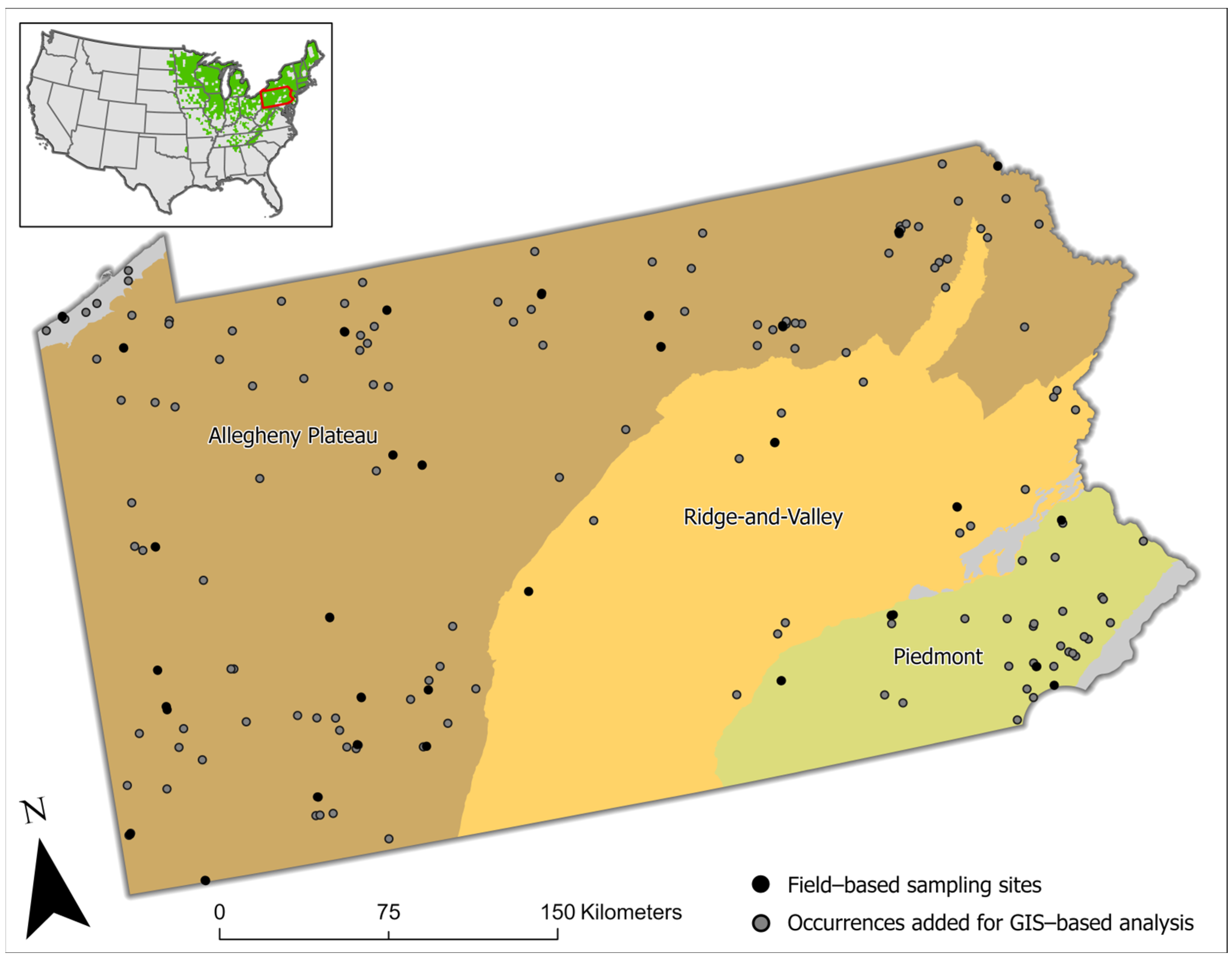
2.1. Study Area

Pennsylvania mainly comprises three physiographic provinces of the Appalachian Mountains (Figure 1). These physiographic provinces, in part, drive climatic variation, with mean annual precipitation ranging from 86–132 cm and mean annual temperatures ranging from 8–14 °C across the state [40]. Climatic and physiographic conditions, in turn, drive floristic diversity across the state. PA is 60% forested, including several forest type groups, of which the broadly defined oak–hickory group dominates southern PA, while maple/beech/birch is most abundant in northern PA [43]. These forest type groups are further classified to include 23 terrestrial and 18 palustrine forest communities [42].
The largest physiographic province in PA, the Allegheny Plateau province, comprises the northern and western parts of the state. This region includes the highest elevations and coldest climates in the state but also warmer climates at lower elevations in southwestern PA [44]. The Allegheny Plateau also contains a high proportion of forested habitat, dominated by broadly defined maple/beech/birch forests in the north, and oak–hickory forests in the southwest [43]. The second largest of these, the Ridge-and-Valley province, runs from southcentral to eastern PA [43]. The Ridge-and-Valley province is characterized by an alternating series of limestone valleys and sandstone ridges. Oak–hickory forests predominate on the infertile sandstone ridges, while the fertile limestone valleys have largely been cleared for agriculture [43]. The smallest physiographic province, the Piedmont, is in southeastern PA and contains some of the most fertile soils and warmest climates in the state. Much of the Piedmont has been cleared for agriculture, although some fragmented forest habitats remain in areas where agriculture is unsuitable [45].

2.2. GIS Methods

2.2.1. Modeling Habitat Suitability

Maxent version 3.3.3 k was used to fit the model through the ‘dismo’ package in R Version 4.2.2 [46,47]. Maxent samples the landscape—defined by environmental covariates—with a set of occurrence points and a set of randomly produced background points. The resulting probability distributions are compared, outputting a final probability distribution based on the principle of maximum entropy [35]. In this study, a probability distribution for ramp habitat suitability was developed using 163 occurrence points mapped against 9877 randomly selected background points across PA. These background points represented a subset of 10,000 initial points minus 123 points that were generated where no data were present for one or more covariates due to features such as streams, lakes, and areas that had been heavily modified by human infrastructure. Although there has been debate about appropriate levels of background sampling in Maxent, predictive performance has been shown to be similar at 1 and 10 times the number of occurrence points as at 10,000 points [48]. Additionally, the default number of 10,000 background points for Maxent has been shown to maximize predictive performance for an area the size of PA in some cases [49].

2.2.2. Occurrence Data Inclusion Criteria

The habitat suitability model included occurrence points distributed across PA (Figure 1). Occurrences were obtained from multiple sources, including a subset of sites in [50] (n = 23), new occurrences visited in 2023 (n = 3), and points obtained from two online databases: iNaturalist (n = 101) and the Global Biodiversity Information Facility (GBIF) (n = 35).
Selection criteria were developed to ensure consistent data quality between field-visited sites and occurrence points taken from online databases. Only verifiable, research-grade iNaturalist observations with public coordinates and location uncertainty distances less than 100 m were used. These points were then visually inspected against an aerial imagery map, and points clearly located within developed spaces were removed. GBIF occurrences derived from iNaturalist observations or with location uncertainty distances greater than 100 m were removed. This cutoff was chosen based on the 90 m resolution of the edaphic and topographic predictor variables, ensuring that occurrence points were within or adjacent to cells containing the ‘true’ environment data values corresponding to the populations they represented. All occurrences were recorded between 2014 and 2023. To reduce the effects of spatial autocorrelation, ‘SDMtoolbox’ [51] was used to rarefy occurrences located within 1 km of one another, which corresponds to the set of environmental predictor variables with the coarsest resolution.

2.2.3. Environmental Predictor Variables

The predictive environment was characterized using 49 predictor variables representing climate, soils, and topography (Table S1). This set of predictor variables was chosen based on those used in the U.S. Forest Service Tree Atlas [52], DISTIB-II [53], and SHIFT [54] to model the distributions of 125 tree species in the eastern U.S. Climatic predictors representing annual trends, seasonality, and extremes of temperature and precipitation from 1970–2000 at 1 km resolution were obtained from WorldClim (https://www.worldclim.org/data/bioclim.html, accessed on 30 October 2024) [44]. Edaphic features representing bedrock geology, as well as physical and chemical properties from the top 30 cm of the soil, were derived from the 10 m resolution Gridded Soil Survey Geographic (https://www.nrcs.usda.gov/resources/data-and-reports/gridded-soil-survey-geographic-gssurgo-database, accessed on 30 October 2024) (gSSURGO) dataset using the gSSURGO ArcToolbox in ESRI ArcMap™ by aggregating soil characteristics for each 10 m pixel from the corresponding map unit key (MUKEY) [55]. A maximum depth of 30 cm was chosen for aggregation to maintain consistency in edaphic representation due to the range in depth of soil profiles. Additionally, ramps have shallow root systems [56,57], lessening the effect of soil properties on ramp growth below this depth. The integrated moisture index was developed by Iverson et al. [58], and other topographic variables, including aspect [59], roughness [60], and topographic position indices [61,62], were derived from a digital elevation model obtained from the PA Department of Conservation and Natural Resources PAMAP program (https://www.pasda.psu.edu/uci/DataSummary.aspx?dataset=1247, accessed on 30 October 2024) [63]. To better link edaphic and topographic predictor variables to the range of conditions within the extent of ramp populations, a 90 m resolution was chosen. Edaphic predictor variables were resampled to 90 m resolution by calculating averages over 3 × 3 10 m pixels using ESRI ArcMAP©. For topographic variables, the 1 m DEM was first resampled to 90 m resolution, and all topographic variables were calculated from the resulting DEM.
After preliminary analysis, the six most influential variables were selected for the final model to reduce overfitting and aid in interpretability (Table 1). Final variables were selected stepwise based on the Pearson correlation coefficient, permutation importance, variable dependency, and biological interpretability (Figure S1). Pearson correlation coefficients among all variables were computed using the ‘ENMTools’ package in R [64]. When correlation coefficients between variables were 0.4 or greater (i.e., exhibiting moderate to high collinearity), the variable with the lower permutation importance was eliminated. All variables with a permutation importance of zero were eliminated regardless of correlation. Finally, variables whose response curves showed dependency were eliminated to aid in the interpretation of biological significance. This process eliminated all but six covariates, which were used to fit the final model.

2.2.4. Model Evaluation

The resulting model was evaluated based on the area under the receiver operating characteristic curve (AUC). AUC is a popular method of model evaluation in the Maxent literature [65] and is interpreted as the probability that a randomly chosen presence location is ranked higher than a randomly chosen background point. The AUC metric ranges from 0.5–1.0; models with AUC values of 0.5 have no predictive ability, while those with AUC values of 1.0 have perfect predictive ability. AUC values are interpreted along the following scale: excellent AUC > 0.90; good 0.80 > AUC < 0.90; fair 0.70 > AUC < 0.80; poor 0.60 > AUC < 0.70; fail 0.50 > AUC < 0.60 [66]. Uncertainty in the AUC metric was evaluated using k-fold cross-validation, which partitions the occurrence data into k subsets. For each subset, the model is trained with k-1 subsets and tested on the kth subset [65]. In this case, k = 5 was chosen based on the sample size. In effect, the 163 occurrence points were randomly partitioned into five subsets, and the model was tested on each subset after using the other subsets to train the model. This allowed for a testing AUC to be computed using independent occurrence data and for the computation of uncertainty metrics, such as standard error, based on differences in model results between each subset [65]. Comparison between training AUC and testing AUC is a useful metric for model performance, assuming an unbiased sample [66]. Individual variable importances were estimated using a jackknife test [67], whereby each variable was excluded in turn and a model was created using the remaining variables. Subsequently, a model was created using each variable in isolation. Through this process, variable importance was evaluated based on model performance when individual variables were excluded or used in isolation in comparison to the overall model.

2.3. Field Methods

2.3.1. Field Sampling Inclusion Criteria

Field sampling was conducted between 2018 and 2021. Populations were included as study sites based on the following criteria: (1) each population occupied at least one acre in size and consisted of at least 1000 ramets; (2) each population exhibited both asexual and sexual recruitment, as evidenced by the presence of all demographic stages (e.g., seedling to adult); (3) populations were distributed throughout all regions of PA to reduce spatial autocorrelation and achieve statewide representation. A total of 30 populations were included in the community data analysis portion of this study and were visited over a three-year period (Figure 1).

2.3.2. Field Sampling

At each site, five plots with 6 m radii were established throughout populations using a subjective (i.e., non-random) approach, aiming to capture the entire range of topographic positions and floristic associates represented at the site. In each plot, elevation, aspect, and topographic position were recorded, and one soil sample was collected from the top 20 cm of soil and within 15 cm of A. tricoccum bulbs (n = 150). This sampling method was used to (1) ensure that samples accurately represented only the localized soil from the rhizosphere; and (2) examine any fine-scale rooting zone variation between plots within each site. Samples were submitted to the Pennsylvania State Agricultural Analytical Services Laboratory (University Park, PA, USA) for chemical analysis. Soil pH was determined using the Water method [68], and macro-nutrient content (available P, K, Ca, Mg) of samples was determined using the Mehlich-3 (ICP) method [69].
Associated flora were documented using a combination of plot and plotless sampling methods. Point-Centered Quarter-Method (PCQM) [70,71] was used to record species and diameter at breast height (1.4 m) of dominant and co-dominant trees and to calculate importance values (IVs) [72,73]. The presence and abundance of understory vegetation, including shrubs, vines, and herbaceous plants, were recorded within a 6 m radius of the plot center using the following scale: (1) one plant observed; (2) 2–10 plants observed; (3) 11–49 plants observed; and (4) 50 or more observed.
Ramps are extensively clonal, often reproducing asexually through bulb division to form large “patches” [56]. The goal of sampling was to capture biotic (floristic associates) and abiotic (edaphic and topographic) features directly within or adjacent to “patches” of ramps. Although the targeted, non-random nature of these sampling methods is prone to bias and may limit extrapolation, it can point to important site conditions and indicators when coupled with GIS-based habitat suitability modeling.

2.3.3. Statistical Analysis of Field Data

Sørenson coefficients (Ss) were calculated to determine the percent similarity of all floristic associates between sites and plots [73]. Sørenson coefficients are calculated using Ss = 2a/(2a + b + c), where “a” is the number of species in both samples and “b” and “c” are the number of species unique to each sample. Binary and presence/absence data were used with a Sørenson (Bray–Curtis) distance measure and city block geometry.
Indicator species analysis (ISA) was used to assess the degree to which a floristic associate is correlated with ramp occurrence given specific site or habitat characteristics. Significance was determined using Dufrêne and Legendre methodology with a Monte Carlo randomization test [27,29]. Floristic abundance data per plot were analyzed based on the following characteristics: region (north, south, east, or west), province (Allegheny Plateau, Piedmont, or Ridge-and-Valley), aspect (N/E/NE/NW, S/W/SW/SE, or flat), and topographic position (floodplain or lower, middle, or upper slope). The significance of floristic associations was evaluated based on a p-value < 0.01. ISA and similarity indices (Sørenson’s coefficient) were calculated using PC-ORD [74].

3. Results

3.1. Model Performance

Three edaphic variables and three topographic variables (Table 1) were used to fit the final model and project habitat suitability across the state (Figure 2). The resulting model had a fair ability to differentiate between suitable and unsuitable habitats, with a training AUC of 0.752. Replicate cross-validation runs had an average testing value of 0.742, with a standard deviation of 0.049 (Figure S2A).

3.2. Topographic Variables

The topographic position index (TPI 2000) was the most important predictor variable, with a percent contribution of 57.8% (Table 1). The jackknife test indicated that when isolated, TPI 2000 contained the best predictive ability and, when removed, resulted in the largest decrease in predictive ability (Figure S2B). TPI 2000 was negatively associated with ramp habitat, as measured by the logistic output. Logistic output decreased from nearly 1.0 (highest suitability) at the lowest topographic positions to just over 0.0 (lowest suitability) at the highest topographic positions (Figure 3).
The integrated moisture index (IMI) was the second most important predictor variable, with a percent contribution of 15.7% (Table 1). IMI was positively associated with ramp suitability, increasing from a logistic output of 0.39 within the driest areas to 0.77 within the wettest areas (Figure 3).
Surface roughness (ROUGH27) had a percent contribution of 11.2% (Table 1) and was negatively correlated with ramp suitability. Logistic output decreased from 0.55 at the smoothest surfaces to just over 0.0 on the roughest surfaces (Figure 3).
In the field, ramp populations were most frequently recorded in bottomland positions (30% of plots) and gradually decreased moving upslope, with 27% of plots recorded in lower slope positions, 23% in middle slope positions, and 20% in upper slope positions (Figure 4). When growing in sloped positions, 77% of plots faced north, east, or northeast, whereas only 10% faced south, west, or southwest. The other 12% of sloped plots faced northwest or southeast.

3.3. Edaphic Variables

Soil depth to bedrock was the most important edaphic predictor, with a percent contribution of 8.3% (Table 1). Logistic output increased linearly from 0.3 within the shallowest soils to 0.55 within the deepest soils (Figure 3).
Bedrock richness was the second most influential edaphic variable on ramp suitability, with a percent contribution of 6.6% (Table 1). Formations high in elements forming base ions such as calcium and magnesium predicted higher suitability (logistic output 0.60) as compared to those of medium (0.49) or low (0.46) base richness (Figure 3).
Silt content was the least important variable included within the model, with a percent contribution of only 0.4% (Table 1). Silt content was positively associated with ramp suitability, but suitability decreased slightly at values greater than 60% (Figure 3).
Soil pH was slightly acidic (5.7), on average, but varied across sites from 4.8 to 7.0. Macronutrients were highly variable, with standard deviations commonly greater than half the value of the mean. Phosphorous averaged 17 ppm, potassium 119, magnesium 170, and calcium 1462 ppm (Table 2).

3.4. Community Analysis

3.4.1. Overall Community Analysis Results

Ramps commonly grew in several rich mesic forest types, including “Tuliptree-Beech-Maple”, “Central Appalachian Rich Cove”, “Sugar maple-Basswood”, and “Sugar maple-Mixed Hardwood Floodplain” [75,76,77,78]. A total of 252 species were recorded in this study: 25 overstory trees, 41 woody understory species, and 186 herbaceous species (Table S2). On average, 50% of species were shared between sites.
Sugar maple (Acer saccharum) was the most important overstory tree, occurring at 90% of sites with an importance value percentage of 32% (Table 3, Table S2). Tulip poplar (Liriodendron tulipifera) and basswood (Tilia americana) ranked second and third, with importance value percentages of 12.8% and 10.6%, respectively. Bitternut hickory (Carya cordiformis) ranked fifth in importance but was a strong indicator on floodplains. Non-native multiflora rose (Rosa multiflora) and Japanese barberry (Berberis thunbergii) were the most common shrubs, occurring at 80% and 63% of sites, respectively. Spicebush (Lindera benzoin) was the most common native woody understory species, occurring at 50% of sites and ranking third in overall abundance (Table 4). The herbaceous layer was dominated by several species of violet (Viola spp.) and bedstraw (Galium spp.), but the single most frequent species was blue cohosh (Caulophyllum thalictroides), followed by yellow trout lily (Erythronium americanum). Several other herbaceous species served as indicators based on region, topographic position, and aspect (Table 5).

3.4.2. Forest Overstory

Sugar maple occurred across the state and was a component of all major forest types where ramps were found. However, several indicators and forest types differed in importance by region. Tulip poplar and American beech were significant indicators in southern PA, particularly the Piedmont, where forests could be classified as “Tuliptree-Beech-Maple” or “Central Appalachian Rich Cove” [76,78]. Sugar maple and black cherry were significant indicators in northern PA, where forests could be classified as “Sugar maple—Basswood” [75].
Bitternut hickory was found on only 21% of ramp plots (Table S2) but was present on 46% of floodplain plots, where it was identified as a statistically significant indicator through ISA (Table 3). Bitternut hickory often played a secondary role in these sites, which are most accurately classified as “Sugar maple—Mixed hardwood Floodplain” forests [77]. However, some sites are better classified as “Bitternut Hickory Floodplain” forest [79], with bitternut hickory occupying a dominant role in the overstory.

3.4.3. Forest Midstory

Two non-native shrub species, multiflora rose and Japanese barberry, were the most common woody understory species encountered at ramp sites. Spicebush was the most frequent native understory woody species, growing at 50% of sites (Table 4). All other native shrub species occurred at less than 50% of sites (Table 4).

3.4.4. Forest Understory

As with the overstory, several regional differences in understory communities were evident. In northern PA, yellow trout lily, white wood aster (Eurybia divaricata), jack-in-the-pulpit (Arisaema triphyllum), broadleaf toothwort (Cardamine diphylla), and purple trillium (Trillium erectum) stood out as indicators. Southern PA had fewer distinct taxa, but both blue cohosh and hairy Solomon’s seal (Polygonatum pubescens) were identified by ISA as statistically significant indicators. Other common associates were sorted by physiographic province. Christmas fern (Polystichum acrostichoides) was an indicator on the Allegheny Plateau, while cut-leaf toothwort (Cardamine concatenata) and wood nettle (Laportea canadensis) were indicators in the Ridge-and-Valley province (Table 5).

4. Discussion

The results of this study of extant wild occurrences can aid in forest farming and in situ planting efforts by pointing to ideal sites for growing ramps. Due to the presence-only methods used in this study, overreliance on individual site characteristics and plant indicators for determining habitat suitability is cautioned. However, taken collectively, model and field results suggest that a suitable ramp habitat is somewhat specific and most strongly governed by moisture availability and soil fertility, and plant community types found at ramp sites are indicative of these same conditions. Climatic variables were found to have no independent predictive ability. The importance of topographic and edaphic predictor variables in relation to climate variables indicates that ramps are well adapted to the entire range of Pennsylvania’s current climate conditions. Indeed, Pennsylvania is well within the core of the geographic distribution of ramps, and they occur throughout the state.

4.1. Topographic Site Factors

This study points to bottomlands or gentle, moist, north- or east-facing lower slopes as the most suitable topographic conditions for growing ramps. The north-to-east-facing slopes encountered in 77% of field plots (Figure 4) receive less intense insolation compared to south-to-west-facing slopes, creating cooler, wetter conditions [80,81]. Likewise, water tables generally sit closer to the surface in bottomlands and lower slope positions, creating moist soil conditions [82]. The response curve for TPI2000 (Figure 4), an indicator for slope position, pointed strongly to the favorability of these low topographic positions. This was confirmed in the field, with a slight majority (57%) (Figure 4) of field plots occurring in bottomlands or on lower slopes.
The response of the integrated moisture index (IMI) also supports the importance of high moisture in ideal ramp-growing locations. The IMI incorporates soil and topographic features, including slope, aspect, cumulative flow of water downslope, landscape curvature, and soil water holding capacity [58]. The positive association between ramps and moist sites in this study follows previous research on their biology and habitat preferences. Ramps, like many members of the Allium genus, have shallow root systems that only penetrate the top 30 cm of soil [23,56,57], and soil moisture has been found to strongly influence ramp growth and survival [8,22].
Gentle slopes were also found to be most suitable for growing ramps. The response curve for surface roughness (ROUGH27) (Figure 3), a measure of the variance in elevation, showed increasing suitability with decreasing surface roughness. The ridges of the Ridge-and-Valley province and steep canyons such as those of the Pine Creek Gorge and West Branch Susquehanna River had the highest levels of surface roughness in PA due to a combination of steep slopes and large reliefs (i.e., large local differences between high and low elevations). The negative association between ramps and these highly rough areas may relate to soil moisture as well; soils on steep slopes are thinner and dry out faster [82], making gently sloping terrain better suited for growing ramps.

4.2. Edaphic Site Factors

Edaphic characteristics in suitable ramp sites varied substantially, but soils in highly suitable sites tended to be derived from base-rich bedrock types such as limestone, dolomite, and calcareous shale (Table S3). At these sites, field measurements indicated that pH and elements forming base ions such as calcium and magnesium were high (Table 2). However, not all ramp sites occurred over base-rich bedrock types, and the observed variation in pH and macronutrients indicates that ramps tolerate a wide range of soil conditions, excluding strongly acidic sites.
The positive association between ramps and base-rich soils is consistent with field experiments finding increased ramp growth and survival rates with the application of calcium fertilizers, particularly those that neutralize aluminum and increase soil pH [8,25]. Fertilizing with slaked lime (Ca(OH)2) has been shown to increase ramp growth and survival in highly acidic soils, making forest farming potentially viable on these sites [25].
While base-rich bedrock types increased suitability only moderately, land use legacy may confound these results. In the Ridge-and-Valley province, limestone and dolomite valleys showed high suitability despite having few ramp occurrences. Soils underlain by these base-rich bedrock types are also well suited to agriculture and have largely been cleared for this purpose [45,83]. It may be that ramps were more abundant in the Ridge-and-Valley province prior to settlement and land clearance, making forested valleys on limestone bedrock in the Ridge-and-Valley province high-quality sites for forest farming establishment.
Ideal soils also tended to be deep and silty. The relationship between soil depth and habitat suitability may be linked to the prevalence of ramps on lower slope positions. These areas receive soil through erosional processes from upslope positions and through depositional processes when streams flood their banks. This combination of colluvium and alluvium creates constructional sites where soil accumulates faster than it erodes, deepening the soil profile over time [82].

4.3. Community Analysis

Plant communities identified in association with ramps were high in overall species richness and shared 50% of species on average, suggesting a similar associated flora. However, many associated plant taxa could be regarded as “generalists” which occur in a variety of habitats including non-forested sites. The presence-only sampling approach used in this study limits the reliability of any single species as an indicator. Instead, plant communities should be used collectively to identify forested habitats suitable for successful introduction of ramps. These plant communities tended to be indicative of rich mesic sites and were consistent with descriptions of a few distinct forest types: “Tuliptree-Beech-Maple”, “Central Appalachian Rich Cove”, “Sugar maple—Basswood” and “Sugar maple—Mixed hardwood Floodplain” [75,76,77,78].
Forest types associated with ramps differed regionally within PA. In the south, forests could be best classified as “Tuliptree-Beech-Maple” or “Central Appalachian Rich Cove”, with a significant presence of Tulip-poplar, American beech, blue cohosh, and hairy Solomon’s seal as identified by ISA (Table 3 and Table 5). The dominance of tulip-poplar on these sites can be explained at least partly by overall regional abundance. It is often dominant on productive mesic sites in southern PA, andis absent in much of the northern part of the state [84]. While not identified as regionally specific, many other species indicative of these forest types also occurred in southern PA. Sugar maple and American basswood were minor overstory components, and cut-leaf toothwort, jack-in-the-pulpit, wood nettle, hairy sweet cicely (Osmorhiza claytonia), Virginia spring beauty (Claytonia virginica), Virginia waterleaf (Hydrophyllum virginianum), great white trillium (Trillium grandiflorum), bloodroot (Sanguinaria canadensis), wood geranium (Geranium maculatum), and others were often present in the understory (Table S2).
In contrast, “Northern hardwood” forests, primarily comprising sugar maple, red maple, black cherry, American beech, and formerly, white ash [75], make up the majority of northern PA. However, the absence of American beech and red maple on ramp sites in northern PA is a notable departure from the traditional concept of “Northern hardwood” forest, and many sites could be more accurately characterized as “Sugar maple—Basswood” or as “Sugar maple—Mixed hardwood Floodplain”, depending on the topographic position. “Sugar maple—Basswood” type forests associated with ramps in this study often occurred on gentle slopes and were dominated by sugar maple and basswood with a black cherry component (Table 3). Understories often included yellow trout lily, broadleaf toothwort, jack-in-the-pulpit, and white wood aster, all of which were identified as significant indicators in northern PA by ISA. Several other herbs were common but not regionally specific, including bloodroot, wood geranium, and Virginia spring beauty. Sugar maple’s high importance as an indicator species in these sites may be a combination of similarities in site preference with ramps and its ability to modify site conditions to facilitate ramp growth. Consistent with its status as an indicator on north-facing slopes (Table 3), sugar maple has a low tolerance for xeric conditions [85]. Additionally, sugar maple leaf litter has a high calcium content [86], which has been shown to positively influence ramp growth and survival [24,25].
Floodplain forests shared sugar maple as a dominant overstory component but also included bitternut hickory as a significant overstory component (Table 3). Bitternut hickory reaches its best size in rich bottomlands [84], and like sugar maple, may modify microsite conditions in favor of ramps. In southern Quebec, Carya species were among those that closed their canopies later, causing more sunlight to reach the understory during the ramp growing season and allowing them to accumulate more carbon, grow wider bulbs, and produce more seeds [87]. However, in stands dominated by bitternut hickory, as in “Bitternut Hickory Floodplain” forest, canopies are often more open, and weedy species dominate the understory [79]. Long-lived and slow-growing forest perennials, including ramps, are more abundant on sites where bitternut hickory plays a secondary role to sugar maple [77], making these sites more favorable for forest farming. Understory herbs commonly found in suitable floodplain sites in this study included purple trillium and Christmas fern, along with many species found in “Sugar maple—Basswood” forests.
These forest types typically occur on sites with topographic and edaphic features identified in this study, namely bottomlands or lower slopes, but sometimes in middle- to upper-slope positions. Soils are typically deep and fertile and are often derived from calcareous parent materials [75,76,77,78]. Other popular herbaceous NTFPs, such as American ginseng (Panax quinquefolius) and goldenseal (Hydrastis canadensis), are also commonly found growing on similar sites [26,88]. However, in this study, ginseng and goldenseal were associated with ramps on only 17% and 10% of sites, respectively (Table S2). These low levels of association could be attributed to a combination of overharvesting in areas where they were formerly associated with ramps and/or differences in climate and soil moisture preferences. Goldenseal is absent from northern PA, where cold winters may limit its viability [88]. Additionally, while goldenseal and ginseng both require mesic soil conditions, growing manuals state their need for good drainage to prevent disease [89,90]. On the other hand, model results and soil moisture measurements point to ramp preference for wet-mesic sites, which remain somewhat moist throughout the year. Despite these differences, forest farming of all three species may be possible in rich sites along a slight moisture gradient.

5. Conclusions

Given current conservation concerns surrounding the exploitation of wild ramp populations, human-assisted conservation activities, including forest farming and other in situ conservation practices, may play a key role as conservation strategies moving forward. The goal of this study was to document habitat conditions associated with ramps for the purpose of guiding forest farming site selection. The targeted, non-random nature of these sampling methods is prone to bias and may limit extrapolation. However, field data and GIS-based habitat suitability modeling provided independent confirmation of the important key site conditions that could be useful in ramp production on forestlands. Maxent modeling suggests that suitable habitat occurs in all regions of the state, but three topographic and three edaphic variables are important: lower slope positions, high moisture index, low surface roughness, deep soil, base-rich bedrock types, and high silt content were all associated with greater suitability. Field data confirmed these observations, with ramp populations growing most commonly on floodplains and lower slopes with north- and east-facing aspects. Soil nutrients varied but were rarely strongly acidic, confirming model results for the suitability of base-rich bedrock types. Several rich moist or mesic forest types predominated, including “Tuliptree-Beech-Maple” and “Central Appalachian Rich Cove” in the south and “Sugar maple—Basswood” or “Sugar maple—Mixed Hardwood Floodplain” in the north.
When taken together, model and field results can be useful to both land managers and owners to guide site selection. Modeled suitability can be used to first narrow down potential sites, namely, forestlands underlain by base-rich bedrock types on moist, gentle lower slope positions and floodplains with deep silty soil. These sites can then be evaluated in the field based on the presence of indicator species assemblages. “Tuliptree-Beech-Maple” or “Central Appalachian Rich Cove” forests dominated by tulip poplar and American beech are characteristic of suitable sites in southern PA, but rich mesic forest indicators, including sugar maple and American basswood, are also present. Blue cohosh and hairy Solomon’s seal are common herbaceous indicators in southern PA, but the additional presence of other rich mesic forest indicators identified by this study may be ideal for successful forest farming establishment. In northern PA, “Sugar maple—Basswood” forests are dominated by sugar maple, basswood, and black cherry, and diverse herbaceous communities, including yellow trout lily, broadleaf toothwort, jack-in-the-pulpit, white wood aster, and other non-regionally specific herbs, are indicative of site suitability. On floodplain sites, “Sugar maple—Mixed Hardwood Floodplain” forests with a component of bitternut hickory in the overstory and with Christmas fern, purple trillium, and other herbs in the understory are indicative of suitability. Finally, soil testing and microsite conditions, such as aspect, can be used to confirm suitability, which is favored on soils that are not strongly acidic and on north- or east-facing slopes.

Supplementary Materials

The following supporting information can be downloaded at: https://www.mdpi.com/article/10.3390/wild1010006/s1. Table S1: List of all variables used in initial Maxent model run; Table S2: Frequency of species identified associating with ramps in Pennsylvania (n = 150 plots); Table S3: Bedrock formations classified by base richness based on dominant lithology; Figure S1: Variable selection process for the ramp suitability model in Maxent; Figure S2: (A) Habitat suitability model test AUC curve for ramps. Specificity is established using predicted area, rather than true commission due to having presence-only data. (B) Jackknife test for variable importance in predicting ramp habitat suitability. Regularized training gain represents how much better the model fits the presence data when compared with a normal distribution. The teal color represents model performance lost when a given variable was removed from the model, while blue represents model performance with that variable alone. Red represents model performance with all variables combined.

Author Contributions

Conceptualization, E.P.B., C.S. and E.H.; methodology, E.P.B., C.S., E.H. and X.C.; software, E.P.B., E.H. and X.C.; validation, E.P.B. and X.C.; formal analysis, E.H.; investigation, E.P.B., C.S. and E.H.; resources, E.P.B. and S.E.N.; data curation, E.P.B., C.S., E.H. and X.C.; writing—original draft preparation, C.S. and E.H.; writing—review and editing, E.P.B., X.C., S.E.N. and E.H.; visualization, E.H.; supervision, E.P.B. and X.C.; project administration, E.H.; funding acquisition, E.P.B. and S.E.N. All authors have read and agreed to the published version of the manuscript.

Funding

This research was funded by The Pennsylvania Department of Conservation and Natural Resources, Wild Resources Conservation Program grant number 18585.

Institutional Review Board Statement

Not applicable.

Informed Consent Statement

Not applicable.

Data Availability Statement

Dataset available on request from the authors.

Conflicts of Interest

The authors declare no conflicts of interest.

References

  1. Baumflek, M.; Chamberlain, J.L. Ramps Reporting: What 70 Years of Popular Media Tells Us About A Cultural Keystone Species. Southeast. Geogr. 2019, 59, 77–96. [Google Scholar] [CrossRef]
  2. Pugh, C. Ramp/Leek “Culture” in Northern Appalachia: A Study of Attitudes, Behaviors, and Knowledge Surrounding a Non-Timber Forest Product. Master’s Thesis, The Pennsylvania State University, University Park, PA, USA, 2022. [Google Scholar]
  3. Moerman, D.E. Native American Food Plants: An Ethnobotanical Dictionary; Timber Press: Portland, OR, USA, 2010. [Google Scholar]
  4. Kofiar, M.; Koyuncu, M.; Bafier, K.H.C. Folk Use of Some Wild and Cultivated Allium Species in Turkey. In Proceedings of the Proceedings of the IVth International Congress of Ethnobotany (ICEB 2005), Istanbul, Turkey, 21–26 August 2005; Volume 87, p. 90. [Google Scholar]
  5. Gębczyński, P.; Bernaś, E.; Słupski, J. Usage of Wild-Growing Plants as Foodstuff. In Cultural Heritage—Possibilities for Land-Centered Societal Development; Hernik, J., Walczycka, M., Sankowski, E., Harris, B.J., Eds.; Environmental History; Springer International Publishing: Cham, Switzerland, 2022; Volume 13, pp. 269–283. ISBN 978-3-030-58091-9. [Google Scholar]
  6. Yamada, T. The Worldview of the Ainu; Columbia University Press: New York, NY, USA, 2001. [Google Scholar]
  7. Rivers, B.; Oliver, R.; Resler, L. Pungent Provisions: The Ramp and Appalachian Identity. Mater. Cult. 2014, 46, 1–24. [Google Scholar]
  8. Bernatchez, A.; Bussières, J.; Lapointe, L. Testing Fertilizer, Gypsum, Planting Season and Varieties of Wild Leek (Allium tricoccum) in Forest Farming System. Agrofor. Syst. 2013, 87, 977–991. [Google Scholar] [CrossRef]
  9. Rock, J.H.; Beckage, B.; Gross, L.J. Population Recovery Following Differential Harvesting of Allium Tricoccum Ait. in the Southern Appalachians. Biol. Conserv. 2004, 116, 227–234. [Google Scholar] [CrossRef]
  10. NatureServe. Allium tricoccum | NatureServe Explorer. Available online: https://explorer.natureserve.org/Taxon/ELEMENT_GLOBAL.2.794001/Allium_tricoccum (accessed on 16 October 2024).
  11. Chamberlain, J.; Beegle, D.; Connette, K. Forest Farming Ramps. Agrofor. Notes 2014, 47, 1–7. [Google Scholar]
  12. Chamberlain, J.L.; Mitchell, D.; Brigham, T.; Hobby, T.; Zabek, L.; Davis, J. Forest Farming Practices. In ASA, CSSA, and SSSA Books; “Gene” Garrett, H.E., Ed.; American Society of Agronomy and Soil Science Society of America: Madison, WI, USA, 2009; pp. 219–255. ISBN 978-0-89118-190-3. [Google Scholar]
  13. Strong, N.; Jacobson, M.G. A Case for Consumer-Driven Extension Programming: Agroforestry Adoption Potential in Pennsylvania. Agrofor. Syst. 2006, 68, 43–52. [Google Scholar] [CrossRef]
  14. McLain, R.; Jones, E. Characteristics of Non-Industrial Private Forest Owners Interested in Managing Their Land for Nontimber Forest Products. J. Ext. 2013, 51, 7. [Google Scholar] [CrossRef]
  15. Dion, P.-P.; Bussières, J.; Lapointe, L. Sustainable Leaf Harvesting and Effects of Plant Density on Wild Leek Cultivation Plots and Natural Stands in Southern Quebec, Canada. Agrofor. Syst. 2016, 90, 979–995. [Google Scholar] [CrossRef]
  16. Nilson, S.E.; Burkhart, E.P.; Jordan, R.T.; Lambert, J.D. Ramp (Allium tricoccum Ait.) Weight Differs across the Harvest Season: Implications for Wild Plant Stewardship and Forest Farming. Agrofor. Syst. 2023, 97, 97–107. [Google Scholar] [CrossRef]
  17. Burkhart, E.P. “Conservation Through Cultivation:” Economic, Socio-Political and Ecological Considerations Regarding the Adoption Of Ginseng Forest Farming In Pennsylvania. Doctoral Dissertation, The Pennsylvania State University, University Park, PA, USA, 2011. [Google Scholar]
  18. Davis, J.; Persons, W.S. Growing and Marketing Ginseng, Goldenseal and Other Woodland Medicinals; New Society Publishers: Gabriola, BC, Canada, 2014. [Google Scholar]
  19. Chamberlain, J.L.; Predny, M. Non-Timber Forest Products: Alternative Multiple-Uses for Sustainable Forest Management. Proc. Enhancing South. Appalach. For. Resour. 2003, 1, 1–6. Available online: https://research.fs.usda.gov/treesearch/9179 (accessed on 30 October 2024).
  20. Weakley, A. Flora of the Southeatern United States: Pennsylvania; University of North Carolina Herbarium, North Carolina Botanical Garden: Chapel Hill, NC, USA, 2023. [Google Scholar]
  21. Rhoads, A.F.; Block, T.A. The Plants of Pennsylvania: An Illustrated Manual; University of Pennsylvania Press: Philadelphia, PA, USA, 2007. [Google Scholar]
  22. Vasseur, L.; Gagnon, D. Survival and Growth of Allium tricoccum AIT. Transplants in Different Habitats. Biol. Conserv. 1994, 68, 107–114. [Google Scholar] [CrossRef]
  23. Geries, L.S.M.; El-Shahawy, T.A.; Moursi, E.A. Cut-off Irrigation as an Effective Tool to Increase Water-Use Efficiency, Enhance Productivity, Quality and Storability of Some Onion Cultivars. Agric. Water Manag. 2021, 244, 106589. [Google Scholar] [CrossRef]
  24. Davis, J.M.; Greenfield, J. Cultivating Ramps: Wild Leeks of Appalachia. In Trends in New Crops and New Uses; ASHS Press: Alexandria, VA, USA, 2002; Volume 1, pp. 449–452. [Google Scholar]
  25. Ritchey, K.D.; Schumann, C.M. Response of Woodland-Planted Ramps to Surface-Applied Calcium, Planting Density, and Bulb Preparation. HortScience 2005, 40, 1516–1520. [Google Scholar] [CrossRef]
  26. Burkhart, E.P. American Ginseng (Panax Quinquefolius L.) Floristic Associations in Pennsylvania: Guidance for Identifying Calcium-Rich Forest Farming Sites. Agrofor. Syst. 2013, 87, 1157–1172. [Google Scholar] [CrossRef]
  27. Peck, J.E. Multivariate Analysis for Ecologists: Step-by-Step, 2nd ed.; MjM Software Design: Gleneden Beach, OR, USA, 2016. [Google Scholar]
  28. Gilliam, F. The Herbaceous Layer in Forests of Eastern North America; Oxford University Press: New York, NY, USA, 2014. [Google Scholar]
  29. Dufrêne, M.; Legendre, P. Species Assemblages and Indicator Species:The Need for a Flexible Asymmetrical Approach. Ecol. Monogr. 1997, 67, 345–366. [Google Scholar] [CrossRef]
  30. Ren, H.; Zhang, Q.; Wang, Z.; Guo, Q.; Wang, J.; Liu, N.; Liang, K. Conservation and Possible Reintroduction of an Endangered Plant Based on an Analysis of Community Ecology: A Case Study of Primulina tabacum Hance in China. Plant Species Biol. 2010, 25, 43–50. [Google Scholar] [CrossRef]
  31. Le Duc, M.G.; Hill, M.O.; Sparks, T.H. A Method for Predicting the Probability of Species Occurrence Using Data from Systematic Surveys. Watsonia 1992, 19, 97–105. [Google Scholar]
  32. Guisan, A.; Zimmermann, N.E. Predictive Habitat Distribution Models in Ecology. Ecol. Model. 2000, 135, 147–186. [Google Scholar] [CrossRef]
  33. Hirzel, A.; Guisan, A. Which Is the Optimal Sampling Strategy for Habitat Suitability Modelling. Ecol. Model. 2002, 157, 331–341. [Google Scholar] [CrossRef]
  34. Bellemare, J.; Motzkin, G.; Foster, D.R. Legacies of the Agricultural Past in the Forested Present: An Assessment of Historical Land-Use Effects on Rich Mesic Forests. J. Biogeogr. 2002, 29, 1401–1420. [Google Scholar] [CrossRef]
  35. Elith, J.; Phillips, S.J.; Hastie, T.; Dudík, M.; Chee, Y.E.; Yates, C.J. A Statistical Explanation of MaxEnt for Ecologists. Divers. Distrib. 2011, 17, 43–57. [Google Scholar] [CrossRef]
  36. Phillips, S.J.; Anderson, R.P.; Schapire, R.E. Maximum Entropy Modeling of Species Geographic Distributions. Ecol. Model. 2006, 190, 231–259. [Google Scholar] [CrossRef]
  37. Yee, T.W.; Mitchell, N.D. Generalized Additive Models in Plant Ecology. J. Veg. Sci. 1991, 2, 587–602. [Google Scholar] [CrossRef]
  38. Busby, J.R. BIOCLIM-a Bioclimate Analysis and Prediction System. Plant Prot. Q. 1991, 6, 8–9. [Google Scholar]
  39. Elith, J.; Graham, C.H.; Anderson, R.P.; Dudík, M.; Ferrier, S.; Guisan, A.; Hijmans, R.J.; Huettmann, F.; Leathwick, J.R.; Lehmann, A.; et al. Novel Methods Improve Prediction of Species’ Distributions from Occurrence Data. Ecography 2006, 29, 129–151. [Google Scholar] [CrossRef]
  40. The Pennsylvania State Climatologist PA Climate Office. Available online: https://climate.met.psu.edu/ (accessed on 22 October 2024).
  41. Pennsylvania Bureau of Topographic and Geologic Survey, Department of Conservation and Natural Resources Bedrock Geology of Pennsylvania 2001. Available online: https://www.dcnr.pa.gov/Geology/PublicationsAndData/Pages/default.aspx (accessed on 30 October 2024).
  42. Pennsylvania Natural Heritage Program Plant Communities of Pennsylvania. Available online: https://www.naturalheritage.state.pa.us/Communities.aspx (accessed on 16 October 2024).
  43. Albright, T.A.; Butler, B.J.; Caputo, J.; Crocker, S.J.; Goff, T.C.; Kurtz, C.M.; Lehman, S.; Lister, T.W.; Luppold, W.G.; Morin, R.S.; et al. Pennsylvania Forests 2019: Summary Report; Resour. Bull. NRS-131; U.S. Department of Agriculture, Forest Service, Northern Research Station: Madison, WI, USA, 2023; Volume 131, pp. 1–36. [CrossRef]
  44. Fick, S.E.; Hijmans, R.J. WorldClim 2: New 1-Km Spatial Resolution Climate Surfaces for Global Land Areas. Int. J. Climatol. 2017, 37, 4302–4315. [Google Scholar] [CrossRef]
  45. Blumberg, B.; Blumberg, B.; Cunningham, R.L. An Introduction to Soils of Pennsylvania; Department of Agriculture and Extension Education: University Park, PA, USA, 1982. [Google Scholar]
  46. Hijmans, R.J.; Phillips, S.; Leathwick, J.; Elith, J.; Hijmans, M.R.J. Package ‘Dismo’. Circles 2017, 9, 1–68. [Google Scholar]
  47. R Core Team, R. R: A Language and Environment for Statistical Computing, Version 4.2.2; R Foundation for Statistical Computing: Vienna, Austria, 2020. [Google Scholar]
  48. Hysen, L.; Nayeri, D.; Cushman, S.; Wan, H.Y. Background Sampling for Multi-Scale Ensemble Habitat Selection Modeling: Does the Number of Points Matter? Ecol. Inform. 2022, 72, 101914. [Google Scholar] [CrossRef]
  49. Phillips, S.J.; Dudík, M. Modeling of Species Distributions with Maxent: New Extensions and a Comprehensive Evaluation. Ecography 2008, 31, 161–175. [Google Scholar] [CrossRef]
  50. Stark, C. Habitat and Flora Associated with Two Ramp/Leek Species (Allium tricoccum and A. burdickii) in Pennsylvania. Master’s Thesis, The Pennsylvania State University, University Park, PA, USA, 2022. [Google Scholar]
  51. Brown, J.L. SDMtoolbox: A Python-Based GIS Toolkit for Landscape Genetic, Biogeographic and Species Distribution Model Analyses. Methods Ecol. Evol. 2014, 5, 694–700. [Google Scholar] [CrossRef]
  52. Peters, M.P.; Prasad, A.M.; Matthews, S.N.; Iverson, L.R. Climate Change Tree Atlas; Version 4; U.S. Forest Service, Northern Research Station and Northern Institute of Applied Climate Science: Delaware, OH, USA, 2020. Available online: https://www.nrs.fs.fed.us/atlas (accessed on 30 October 2024).
  53. Iverson, L.R.; Peters, M.P.; Prasad, A.M.; Matthews, S.N. Analysis of Climate Change Impacts on Tree Species of the Eastern US: Results of DISTRIB-II Modeling. Forests 2019, 10, 302. [Google Scholar] [CrossRef]
  54. Iverson, L.R.; Prasad, A.M.; Peters, M.P.; Matthews, S.N. Facilitating Adaptive Forest Management under Climate Change: A Spatially Specific Synthesis of 125 Species for Habitat Changes and Assisted Migration over the Eastern United States. Forests 2019, 10, 989. [Google Scholar] [CrossRef]
  55. Soil Survey Staff. Gridded Soil Survey Geographic (gSSURGO) Database for the United States of America and the Territories, Commonwealths, and Island Nations Served by the USDA-NRCS; Natural Resources Conservation Service: Lincoln, NE, USA, 2014. [Google Scholar]
  56. Nault, A.; Gagnon, D. Ramet Demography of Allium Tricoccum, A Spring Ephemeral, Perennial Forest Herb. J. Ecol. 1993, 81, 101–119. [Google Scholar] [CrossRef]
  57. Sitepu, B.S. An Integrative Taxonomic Study of Ramps (Allium tricoccum Aiton) Complex. Master’s Thesis, Ohio University, Athens, OH, USA, 2018. [Google Scholar]
  58. Iverson, L.R.; Dale, M.E.; Scott, C.T.; Prasad, A. A Gis-Derived Integrated Moisture Index to Predict Forest Composition and Productivity of Ohio Forests (U.S.A.). Landsc. Ecol. 1997, 12, 331–348. [Google Scholar] [CrossRef]
  59. Beers, T.W.; Dress, P.E.; Wensel, L.C. Notes and Observations: Aspect Transformation in Site Productivity Research. J. For. 1966, 64, 691–692. [Google Scholar]
  60. Riley, S.J.; DeGloria, S.D.; Elliot, R. Index That Quantifies Topographic Heterogeneity. Intermt. J. Sci. 1999, 5, 23–27. [Google Scholar]
  61. Weiss, A. Topographic Position and Landforms Analysis. In Proceedings of the Poster Presentation, ESRI User Conference, San Diego, CA, USA, 9-13 July 2001; Volume 200. [Google Scholar]
  62. Jenness, J.; Majka, D.; Beier, P. Corridor Designer Evaluation Tools; Northern Arizona University: Flagstaff, AZ, USA, 2011; Available online: https://www.jennessent.com/arcgis/corridor.htm (accessed on 30 October 2024).
  63. PAMAP Program, PA Department of Conservation and Natural Resources, Bureau of Topographic and Geologic Survey. PAMAP Program 3.2 Ft Digital Elevation Model of Pennsylvania. 2008. Available online: https://www.pasda.psu.edu/uci/datasummary.aspx?dataset=1247 (accessed on 30 October 2024).
  64. Warren, D.L.; Matzke, N.J.; Cardillo, M.; Baumgartner, J.B.; Beaumont, L.J.; Turelli, M.; Glor, R.E.; Huron, N.A.; Simões, M.; Iglesias, T.L.; et al. ENMTools 1.0: An R Package for Comparative Ecological Biogeography. Ecography 2021, 44, 504–511. [Google Scholar] [CrossRef]
  65. Merow, C.; Smith, M.J.; Silande, J.A., Jr. A Practical Guide to MaxEnt for Modeling Species’ Distributions: What It Does, and Why Inputs and Settings Matter. Ecography 2013, 36, 1058–1069. [Google Scholar] [CrossRef]
  66. Araújo, M.B.; Pearson, R.G.; Thuiller, W.; Erhard, M. Validation of Species–Climate Impact Models under Climate Change. Glob. Chang. Biol. 2005, 11, 1504–1513. [Google Scholar] [CrossRef]
  67. Phillips, S.J. A Brief Tutorial on Maxent. Att Res. 2005, 190, 231–259. [Google Scholar]
  68. Eckert, D.; Sims, J.T. Recommended Soil pH and Lime Requirement Tests. Recomm. Soil Test. Proced. Northeast. U.S. Northeast Reg. Bull. 1995, 493, 11–16. [Google Scholar]
  69. Wolf, A.M.; Beegle, D.B. Recommended Soil Tests for Macronutrients: Phosphorus, Potassium, Calcium, and Magnesium. Recomm. Soil Test. Proced. Northeast. U.S. Northeast Reg. Bull 1995, 493, 25–34. [Google Scholar]
  70. Causton, D.R. An Introduction to Vegetation Analysis; Springer: Dordrecht, The Netherlands, 1988; ISBN 978-0-04-581025-3. [Google Scholar]
  71. Kent, M. Vegetation Description and Data Analysis: A Practical Approach; John Wiley & Sons: New York, NY, USA, 2011. [Google Scholar]
  72. Curtis, J.T.; McIntosh, R.P. An Upland Forest Continuum in the Prairie-Forest Border Region of Wisconsin. Ecology 1951, 32, 476–496. [Google Scholar] [CrossRef]
  73. Anderson, M.J. Analysis of Ecological Communities: Bruce McCune and James B. Grace, MjM Software Design, Gleneden Beach, USA, 2002, ISBN 0 9721290 0 6, US$ 35 (Pbk). J. Exp. Mar. Biol. Ecol. 2003, 289, 303–305. [Google Scholar] [CrossRef]
  74. McCune, B.; Mefford, M.J. PC-ORD Multivariate Analysis of Ecological Data, Version 6; MjM Software Design: Gleneden Beach, OR, USA, 2011. [Google Scholar]
  75. Fike, J. Terrestrial & Palustrine Plant Communities of Pennsylvania; Bureau of Forestry, PA, Department of Conservation and Natural Resources: Harrisburg, PA, USA, 1999. [Google Scholar]
  76. NatureServe. Central Appalachian Rich Cove Forest | NatureServe Explorer. Available online: https://explorer.natureserve.org/Taxon/ELEMENT_GLOBAL.2.687966/Acer_saccharum_-_Fraxinus_americana_-_Tilia_americana_-_Liriodendron_tulipifera_-_Actaea_racemosa_Forest (accessed on 16 October 2024).
  77. Zimmerman, E. Sugar Maple—Mixed Hardwood Floodplain Forest Factsheet. Pennsylvania Natural Heritage Program. 2022. Available online: https://www.naturalheritage.state.pa.us/Community.aspx?=30017 (accessed on 30 October 2024).
  78. Zimmerman, E.; Fike, J. Tuliptree—Beech—Maple Forest Factsheet. Pennsylvania Natural Heritage Program. 2022. Available online: https://www.naturalheritage.state.pa.us/Community.aspx?=16065 (accessed on 30 October 2024).
  79. Perles, S. Bitternut Hickory Floodplain Forest Factsheet. Pennsylvania Natural Heritage Program. 2022. Available online: https://www.naturalheritage.state.pa.us/Community.aspx?=30003 (accessed on 30 October 2024).
  80. Osman, N.; Barakbah, S.S. The Effect of Plant Succession on Slope Stability. Ecol. Eng. 2011, 37, 139–147. [Google Scholar] [CrossRef]
  81. Nevo, E.; Fragman, O.; Dafni, A.; Beiles, A. Biodiversity and interslope divergence of vascular plants caused by microclimatic differences at “evolution canyon”, lower nahal oren, mount carmel, Israel. Isr. J. Plant Sci. 1999, 47, 49–59. [Google Scholar] [CrossRef]
  82. Randall, J.; Anderson, S. Soils Genesis and Geomorphology; Cambridge University Press: Cambridge, UK, 2005; p. 832. ISBN 521812011. [Google Scholar]
  83. Fletcher, S.W. The Expansion of the Agricultural Frontier. Pa. Hist. J.-Atl. Stud. 1951, 18, 119–129. [Google Scholar]
  84. Burns, R.M.; Honkala, B.H. Silvics of North America: Volume 2. Hardwoods; U.S. Department of Agriculture, Farm Service Agency: Washington, DC, USA, 1990.
  85. Caspersen, J.P.; Kobe, R.K. Interspecific Variation in Sapling Mortality in Relation to Growth and Soil Moisture. Oikos 2001, 92, 160–168. [Google Scholar] [CrossRef]
  86. Ott, N.F.J.; Watmough, S.A. Contrasting Litter Nutrient and Metal Inputs and Soil Chemistry among Five Common Eastern North American Tree Species. Forests 2021, 12, 613. [Google Scholar] [CrossRef]
  87. Dion, P.-P.; Bussières, J.; Lapointe, L. Late Canopy Closure Delays Senescence and Promotes Growth of the Spring Ephemeral Wild Leek (Allium tricoccum). Botany 2017, 95, 457–467. [Google Scholar] [CrossRef]
  88. Houston, E. Habitat Modeling of Goldenseal (Hydrastis canadensis L.) and Ramps (Allium tricoccum ait.): Implications for In Situ Conservation and Guidance for Forest Cultivation. Master’s Thesis, The Pennsylvania State University, University Park, PA, USA, 2024. [Google Scholar]
  89. Davis, J.; McCoy, J.-A. Commercial Goldenseal Cultivation | NC State Extension Publications. Available online: https://content.ces.ncsu.edu/commercial-goldenseal-cultivation (accessed on 16 October 2024).
  90. Carroll, C.; Apsley, D. Growing American Ginseng in Ohio: An Introduction. Ohio State University Extension. 2004. Available online: https://ohioline.osu.edu/factsheet/F-56 (accessed on 30 October 2024).
Figure 1. Ramp sampling sites and occurrences added for GIS-based analysis across Pennsylvania. Distribution of ramps in the contiguous US shown in inset.
Wild 01 00006 g001
Figure 2. The Maxent model projected onto the environmental variables with occurrence points. Warmer colors show areas with a higher predicted suitability for ramps.
Wild 01 00006 g002
Figure 3. Response curves for variables used in the Maxent model. Curves show how the logistic prediction changes as each environmental variable is varied, keeping all other environmental variables at their average sample value. The mean response of the 5 replicate Maxent runs is in red, and the mean +/− one standard deviation is in blue (blue and green for categorical variables).
Wild 01 00006 g003
Figure 4. Topographic positions and aspects associated with ramps in Pennsylvania.
Wild 01 00006 g004
Table 1. Predictor variables used to develop the habitat suitability model in Maxent.
VariableDescriptionPercent ContributionSource
Topographic predictors
TPI2000Topographic position index (2000 m neighborhood)57.8PA Department of Conservation and Natural Resources
ROUGH27Variance of elevation (27-pixel neighborhood)11.2PA Department of Conservation and Natural Resources
IMIIntegrated moisture index15.7Iverson et al., 1997 [58]
Edaphic predictors
DEPTHSoil depth to underlying bedrock8.3USDA Natural Resource Conservation Service
FORMATIONSFertility of bedrock formations6.6PA Department of Conservation and Natural Resources
SILT% Silt0.4USDA Natural Resource Conservation Service
Table 2. Soil summary data from ramp populations in Pennsylvania.
NutrientsMean (SD)Range
pH5.7 (0.6)4.8–7.0
P (ppm)17 (13)5–76
K (ppm)119 (42)44–269
Mg (ppm)170 (124)60–721
Ca (ppm)1462 (752)356–3399
Table 3. Relative abundances and importance value percentages (IV%) for dominant or co-dominant overstory tree species associated with ramps in Pennsylvania, along with indicator species analysis (ISA) results.
Scientific Name +Common NameRelative AbundanceIV %ISA
Freq.Den.Dom.LatProvAspectTopo
Acer saccharum MarshallSugar maple28.43929.732.4%N **AP ***N **
Liriodendron tulipifera L.Tulip poplar8.310.319.812.8%S ***P ***
Tilia americana L.American basswood12.310.88.610.6%
Prunus serotina Ehrh.Black cherry9.68.57.78.6%N **
Carya cordiformis (Wang) K. KochBitternut hickory7.676.16.9% Flat **F ***
Quercus rubra L.Northern red oak6.64.78.56.6%
Fagus grandifolia Ehrh.American beech4.93.73.84.1%S ***P ***
Fraxinus americana L.White ash3.92.73.63.4%
Ulmus rubra Muhl.Slippery elm2.922.22.4%
Carya ovata (P. Miller) K. KochShagbark hickory2.921.22.1%
Quercus alba L.White oak1.721.21.6%
Platanus occidentalis L.American sycamore0.812.11.3%
Juglans nigra L.Black walnut1.21.71.11.3%
Acer rubrum L.Red maple1.21.50.91.2%
Betula alleghaniensis Britt.Yellow birch11.50.61.0%
Betula lenta L.Black birch0.81.20.50.9%
Carya tomentosa Sarg.Mockernut hickory0.50.71.20.8%
Robinia pseudoacacia L.Black locust0.50.50.40.5%
Tsuga canadensis (L.) CarrièreEastern hemlock0.30.50.20.4%
Carya glabra MillerPignut hickory0.30.50.20.3%
Quercus montana Willd.Chestnut oak0.20.20.20.2%
Magnolia acuminata L.Cucumber magnolia0.20.20.20.2%
Sassafras albidum (Nutt.) NeesSassafras0.20.20.20.2%
Ulmus americana L.American elm0.20.20.10.2%
Carya sp. Nutt.Hickory species0.20.20.10.2%
Significance denoted by p < 0.001 ***, p < 0.01 **. Latitude: north (N) and south (S); longitude: west (W) and east (E). Physiographic provinces: Appalachian Plateau (AP), Piedmont (P), and Ridge-and-Valley (RV). Aspect: N/E/NE/NW (N), S/W/SW/SE (S), and Flat (F). Topographic position: lower slope (L), middle slope (M), upper slope (U), and floodplain (F). + All taxonomy follows Weakley, 2023 [20].
Table 4. The 20 most frequent (ranked by site) woody understory species associated with ramps in Pennsylvania.
Scientific Name +Common Name% of Sites and (n)
Rosa multiflora Thunb. Ex. Murr. *Multiflora rose80 (24)
Berberis thunbergii A.P. de Candolle *Japanese barberry63 (19)
Lindera benzoin (L.) BlumeSpicebush50 (15)
Ribes sp. L.Gooseberry47 (14)
Rubus sp. L.Blackberry 47 (14)
Sambucus racemosa L. var. pubens (Michx.) Trautv. & C.A. MeyRed elderberry43 (13)
Hamamelis virginiana L.Witch-hazel37 (11)
Prunus virginiana L.Choke cherry33 (10)
Vitis sp. L.Grape vine33 (10)
Toxicodendron radicans (L.) KuntzePoison ivy27 (8)
Carpinus caroliniana WalterMusclewood27 (8)
Parthenocissus quinquefolia (L.) Planch.Virginia creeper23 (7)
Ostrya virginiana (P. Miller) K. KochAmerican hophornbeam23 (7)
Rubus phoenicolasius Maxim. *Wineberry20 (6)
Viburnum prunifolium L.Blackhaw20 (6)
Celastrus orbiculatus Thunb. *Oriental bittersweet17 (5)
Crataegus sp. L.Hawthorn 17 (5)
Lonicera morrowii A. Gray or bella Zabel *Morrow’s or Bell’s honeysuckle17 (5)
Lonicera maackii (Rupr.) Herder *Amur honeysuckle13 (4)
Elaeagnus umbellata Thunb. *Autumn olive13 (4)
Asterisk (*) denotes non-native, exotic species. + All taxonomy follows Weakley, 2023 [20].
Table 5. The 20 most frequent (ranked by site) herbaceous species associated with ramps in Pennsylvania, including statistically significant indicator species analysis (ISA) results.
Scientific Name +Common Name% of Sites and (n)ISA
LatLongProvAspectTopo
Caulophyllum thalictroides. (L.) Michx.Blue cohosh83 (25)S **W *** N **
Erythronium americanum Ker-Gawl.Yellow trout lily83 (25)N ***
Podophyllum peltatum L.Mayapple80 (24)
Polystichum acrostichoides (Michx.) Schott Christmas fern77 (23) AP **
Eurybia divaricata (L.) G.L. Nesom White wood aster73 (22)N **E ***
Dryopteris intermedia (Muhl. Ex Willd.) A. GrayIntermediate woodfern70 (21) W ***
Osmorhiza claytonii (Michx.) C. B. Clarke Hairy sweet cicely 70 (21)
Circaea canadensis (L.) HillEnchanter’s nightshade70 (21) E *** Flat **F **
Polygonatum pubescens (Willd.) Pursh.Hairy Solomon’s seal70 (21)S **
Alliaria petiolata (Bieb.) Cavara & Grande *Garlic mustard67 (20)
Arisaema triphyllum (L.) SchottJack-in-the-pulpit67 (20)N **E ** F **
Cardamine diphylla (Michx.) Alph. WoodBroadleaf toothwort67 (20)N ***W **AP **
Persicaria virginiana (L.) Gaert.Jumpseed67 (20)
Geum canadense JacquinWhite avens67 (20)
Maianthemum racemosum (L.) LinkFalse Solomon’s seal67 (20) Flat **
Impatiens spp.Jewelweed (any species)66 (20)
Cardamine concatenata (Michx.) O. SchwarzCut-leaf toothwort63 (19) W **RV **
Viola sororia Willde.Common blue violet63 (19) F **
Trillium erectum L.Purple trillium60 (18)N **W ***AP **
Laportea canadensis (L.) Wedd. Wood nettle56 (17) RV **
Asterisk (*) denotes non-native, exotic species. Significance denoted by p < 0.001 ***, p < 0.01 **. Latitude: north (N) and south (S) Longitude: west (W) and east (E). Physiographic provinces: Appalachian Plateau (AP), Piedmont (P), and Ridge-and-Valley (RV). Aspect: N/E/NE/NW (N), S/W/SW/SE (S), and Flat (F). Topographic position: lower slope (L), middle slope (M), upper slope (U), and floodplain (F). Excludes Galium spp., Viola spp., and Dryopteris spp., for which several unidentified species were frequent. + All taxonomy follows Weakley, 2023 [20].
Disclaimer/Publisher’s Note: The statements, opinions and data contained in all publications are solely those of the individual author(s) and contributor(s) and not of MDPI and/or the editor(s). MDPI and/or the editor(s) disclaim responsibility for any injury to people or property resulting from any ideas, methods, instructions or products referred to in the content.

