Abstract
We continue Riemann’s program of geometrizing physics, extending it to encompass gravitational and electromagnetic fields as well as media, all of which influence the geometry of spacetime. The motion of point-like objects—both massive and massless—follows geodesics in this modified geometry. To describe this geometry, we generalize the notion of a metric to local scaling functions which permit not only quadratic but also linear dependence on temporal and spatial separations. Our local scaling functions are defined on flat spacetime coordinates. We demonstrate how to construct various geometries directly from field sources, using symmetry and superposition, without relying on field equations. For each geometry, two key visualizations elucidate the connection between the geometry and the dynamics as follows: (1) the cross-sections of the ball of admissible velocities, and (2) the cross-sections of the local scaling function.
Keywords:
geometrization in relativity; local scaling function; admissible velocities domain; relativistic dynamics; superposition in gravity MSC:
58E10; 53C22; 51-02; 49S05; 51P05; 78-10; 83D05
1. The Geometric Description of Physics
One of the fundamental laws of classical physics is the Law of Inertia, first introduced by Galileo Galilei. This law states that an “object at rest or in motion with constant velocity will remain in that state unless acted upon by an external force”. The motion of such an object is called uniform motion, or free motion, where “free” means free of outside influences. The Law of Inertia is based on the fact that an inanimate object cannot change its velocity on its own accord. Thus, once its velocity is constant, it will remain constant in the absence of external forces.
To express this law mathematically, we need to introduce a three-dimensional spatial coordinate system and a clock so that we may describe the object’s trajectory, that is, its position at any given time t. If, for example, the object moves with constant velocity , then its trajectory is , where is the object’s initial position at time . The graph of the object’s trajectory is known as its worldline. When is constant, as above, the object’s worldline is a straight line
in a four-dimensional spacetime with coordinates .
The Law of Inertia has thus revealed a deep connection between the physical concept of free motion and a geometric object—a straight line in spacetime. In what follows, we will extend this connection to the case where there are external forces at play.
Galileo’s Principle of Relativity, another fundamental law of classical physics, states that the laws of physics must be the same in all inertial frames of reference. In essence, this principle consists of the following two different, but equally important statements:
- The same experiment, when observed from different inertial frames, will lead to the same physical laws.
- The same experiment, when performed in different inertial frames, will yield the same results.
The Principle of Relativity requires the invariance of physical laws under the transformations between inertial frames. Thus, it is natural to use transformational geometry in physics. In fact, classical physics requires invariance under the Galilean transformations, formulated by Galileo himself.
The first person to propose a geometric approach to physics was Bernhard Riemann (1826–1866) [1]. Riemann is better known for his work in mathematics, but he became interested in physics in his early twenties. His goal was to create a single mathematical framework that covered gravitation, light, electricity, and magnetism. In 1894, Felix Klein said the following:
“I must mention, first of all, that Riemann devoted much time and thought to physical considerations. Grown up under the tradition which is represented by the combinations of the names of Gauss and Wilhelm Weber, influenced on the other hand by Herbart’s philosophy, he endeavored again and again to find a general mathematical formulation for the laws underlying all natural phenomena …. The point to which I wish to call your attention is that these physical views are the mainspring of Riemann’s purely mathematical investigations [2]”.
Riemann perceived physics through a geometric lens. He generalized the concept of straight lines to geodesics, an idea destined to be fundamental in Einstein’s General Relativity (). As noted in [3], “one of the main features of the local geometry conceived by Riemann is that it is well suited to the study of gravity and more general fields in physics”. Riemann believed that the forces acting on a system determine its geometry—for Riemann, force was geometry.
The application of Riemannian mathematics to gravity, however, required two key developments. First, while Riemann considered how forces influence three-dimensional space, relativistic physics is conducted in four-dimensional spacetime. One must analyze trajectories in spacetime, not just in space. As we saw above, an object moves with constant velocity if and only if its four-dimensional worldline is a straight line. In contrast, knowing that an object moves along a straight line in three-dimensional space provides no information about whether it is accelerating. As Minkowski famously stated: “Henceforth, space by itself and time by itself, are doomed to fade away into mere shadows, and only a kind of union of the two will preserve an independent reality [4]”. In the early twentieth century, the Lorentz transformations replaced the Galilean transformations between inertial frames, since neither the speed of light nor Maxwell’s Equations (the equations of electromagnetism) are preserved by the Galilean transformations. It is generally accepted that Lorentz transformations are the true spacetime transformations between inertial frames.
Riemann worked solely with positive-definite metrics. However, the Minkowski metric of flat spacetime (see below) is not positive-definite – it is pseudo-Riemannian. The exploration of pseudo-Riemannian geometry was a crucial step in the development of .
In 1915, fifty years after Riemann’s death, Albert Einstein made pseudo-Riemannian geometry the foundation of . Acknowledging Riemann’s influence, Einstein said:
“However, the physicists were still far removed from such a way of thinking; space was still, for them, a rigid, homogeneous something, incapable of changing or assuming various states. Only the genius of Riemann, solitary and uncomprehended, had already won its way to a new conception of space, in which space was deprived of its rigidity, and the possibility of its partaking in physical events was recognized. This intellectual achievement commands our admiration all the more for having preceded Faraday’s and Maxwell’s field theory of electricity [5]”.
At its core, is a direct realization of Riemann’s principle that "force equals geometry". In , the gravitational force is not treated as an external interaction but rather as the curvature of spacetime itself. The curving of the spacetime is described by a metric on a four-dimensional pseudo-Riemannian manifold, and the metric is derived from Einstein’s field equations. According to the Equivalence Principle, an object’s acceleration in a gravitational field is independent of its mass, implying that curved spacetime provides a universal stage on which all objects move. In other words, gravity shapes the geometry of spacetime in the same way for all objects.
However, represents only a partial fulfillment of Riemann’s vision. The Equivalence Principle does not apply to the electromagnetic (EM) force. The EM force on a charged particle depends on its charge-to-mass ratio. Unlike gravity, the EM field does not create a universal stage—its effect varies from one test particle to another. Indeed, a neutral particle feels no EM force at all. This distinction between gravity and EM was also recognized in the geometric approach of [6].
In this paper, we present our geometric approach to relativistic physics. To describe the motion of point-like objects, our underlying state space is Minkowski space M (see Section 3 for details), and our transformation group is a spin-1 representation of the Lorentz group. In [7], a local scaling function () was introduced as a new geometric tool to describe infinitesimal distances between points in spacetime. The resulting geometry unifies electromagnetism and gravity, propagation in media, and even some quantum effects. The original version of our unification theory appears in a recent book [8] but has evolved since its publication. Since many physical applications of geometry do not necessarily require a manifold-based description, our approach will use only a linear space background.
We emphasize that, in this paper, we describe the motion of point-like objects alone. That is, objects which have no internal rotation. As a result, we obtain all of our results using real Minkowski space. In an upcoming paper, we will work in complexified Minkowski space in order to incorporate spin. Some preliminary results appear in [8].
For us, a geometry means the following:
- An inertial frame of an observer, far away from the sources of the field, for labelling events.
- A representation of the Lorentz group, to satisfy the Principle of Relativity and ensure the Lorentz covariance of the model.
- A local scaling function to describe the influence of fields and media on distances.
Local scaling functions offer a powerful tool for visualizing geometry. By examining the cross-sections of an , we can observe the force and momentum imparted by the field on an object. Additionally, define the ball of admissible velocities, which determines the speed of light in the spacetime influenced by the field. Furthermore, we can visualize the field’s effect on the hyperboloid of four-velocities, providing deeper insight into how the field shapes motion and dynamics.
Other authors have described geometry through various frameworks that extend beyond the traditional metric-based definitions. One prominent approach is conformal and affine geometries, which focus on the relationships between points, lines, and angles within a given set, without necessarily relying on a distance metric. As we will see later, these geometries also play a role in relativistic physics. Weyl geometry integrates both a metric tensor and a scalar field to describe gravitational phenomena. In this formulation, the gravitational field is not solely determined by the metric but also incorporates a geometrical scalar field, providing a broader perspective on geometric structures [9]. Derived geometry offers a categorical approach that generalizes traditional manifold theory. This framework allows geometric properties to be studied without relying on conventional metric structures [10].
2. Extending Riemann’s Program—Unifying Gravity and Electromagnetism
In this paper, we examine the following fundamental question: Can Riemann’s principle that “force equals geometry” be extended beyond gravity? Specifically, is it possible to construct a geometric framework that handles gravity and object-dependent forces, such as electromagnetism?
To explore this, we introduce new concepts that extend the geometrization of physics beyond gravity, incorporating electromagnetism, motion in media, and even certain aspects of quantum behavior. The model we present serves as a natural continuation of Riemann’s program, further advancing the geometric interpretation of physical forces.
Different forces produce different trajectories, and we employ a variational principle to determine the stationary or “shortest” paths that objects follow through spacetime.
“Many results in both classical and quantum physics can be expressed as variational principles, and it is often when expressed in this form that their physical meaning is most clearly understood. Moreover, once a physical phenomenon has been written as a variational principle, … it is usually possible to identify conserved quantities, or symmetries of the system of interest, that otherwise might be found only with considerable effort [11]”.
In pseudo-Riemannian geometry, the distance between two infinitesimally close spacetime points depends quadratically on their temporal and spatial separations. This assumption, rooted in the Pythagorean Theorem and its generalizations, appears reasonable for describing gravity. However, when dealing with the electromagnetic field, a purely quadratic dependence is insufficient—a linear dependence on displacements is required. Traditionally, the quadratic structure was justified by the need to ensure the positive definiteness of the metric. However, since we work with non-positive-definite metrics, there is no fundamental reason to exclude a simpler, linear dependence.
We will construct geometries which incorporate both linear and quadratic dependence. To determine distances in spacetime, we introduce local scaling functions. These functions include both linear and quadratic dependencies. This modification allows us to treat other forces in addition to gravity. Our geometries are also object dependent. By allowing the geometry to depend on a test charge’s charge-to-mass ratio and on a photon’s frequency, we can naturally incorporate electromagnetism and the motion of light in media into our model. The broadening of the concept of geometry to include linear dependence and object-dependent effects not only extends Riemann’s program but also provides a unified geometric foundation for physical phenomena due to different forces.
3. The Geometry of Minkowski Space
To simplify the theory, we represent the motion of objects as observed in inertial frames. These are frames of reference in which both an accelerometer and a gyroscope at rest measure zero. It is not necessary to be familiar with these devices. It is enough to imagine an observer far away from the sources of the field. The observer’s position is the origin of our inertial frame. In this frame, we establish the spacetime coordinates . Sometimes we will label the coordinates , where . In this way, all have dimensions of length. Here, c is the speed of light in vacuum. In what follows, we work with units in which .
We begin by considering the motion of point-like objects. The motion of the object is described by its worldline, namely a function , where is some evolution parameter. At this point, we must distinguish between spacetime positions and four-vectors. A spacetime position is a 4-tuple representing the spacetime coordinates of an event. A translation is a function T which acts on spacetime points and has the form
where are constants that are not all equal to 0. For any spacetime point and any translation T, we clearly have . That is, spacetime points are not invariant under translations.
On the other hand, the separation of two spacetime points x and y is invariant under translations. We extend the translation T, which acts on spacetime points, to , which acts on separations, by . Then, we have
Thus, the separation of spacetime points is an example of a four-vector, a quantity which is invariant under translations. Another example of a four-vector is the four-velocity, defined as follows. Let be the worldline of a moving object. The object’s four-velocity with respect to , denoted by , is defined by
Since the four-velocity is a limit of four-vectors, it is also a four-vector. The four-acceleration with respect to , denoted by and defined by , is also a four-vector.
Newtonian dynamics uses the Principle of Relativity but with respect to the Galilean transformations. Under these transformations, the acceleration of an object is invariant across inertial frames, and Newton’s laws are statements about accelerations. For most applications, Newtonian dynamics is a very good approximation, and it is still used today in the majority of technologies.
Nevertheless, experiments in the early twentieth century indicated that certain physical laws were not invariant under Galilean transformations. This included Maxwell’s equations, the main equations of electrodynamics, which are invariant under the Poincaré transformations. This led Einstein [12,13] to conclude that the group of Poincaré transformations [4] are the true spacetime transformations between inertial frames, while Galilean transformations are only an approximation. Thus, the laws of physics needed to be modified to satisfy the Principle of Relativity with respect to the Poincaré transformations.
The Poincaré transformations include the spacetime translations (2) and the linear subgroup of Lorentz transformations. The Lorentz group contains rotations and boosts. The rotations act like the orthogonal group on the spatial part of a spacetime position or four-vector and leave the time component unchanged. Boosts are transformations from one inertial frame to another inertial frame, moving with some fixed velocity with respect to the first frame. For example, the Lorentz transformation from a frame K to a frame , with constant velocity with respect to K, is a boost in the x direction and is given by
where . Under the Poincaré transformations, Maxwell’s Equations are invariant, and the speed of light is the same in all inertial frames. By custom, theories which are invariant under the Poincaré transformations are called Lorentz covariant.
There is also a Lorentz-invariant metric [8,14], , called the Minkowski metric. The Minkowski interval between two events with infinitesimal displacements is defined by
Here, we use Einstein’s summation convention, expressed as follows: whenever an index appears twice in a single term (once as an upper index and once as a lower index), it is implicitly summed over all possible values of that index. The interval (6) is invariant under the Lorentz transformations. Moreover, the Lorentz transformations are sometimes defined to be the transformations that preserve this interval.
For any two four-vectors and , we define a Lorentz-invariant Minkowski dot product by
The length of a four-vector a is . Note that the Minkowski dot product is not positive definite. A four-vector a is timelike, null or spacelike if is positive, zero, or negative, respectively. Since the speed of massive objects is less than the speed of light, the interval between two points on an object’s worldline is timelike. Light travels along null vectors. Spacelike vectors do not represent displacement during real motion.
We formally define Minkowski space, or flat spacetime, as the set , equipped with the Minkowski metric, the Minkowski dot product, and the Lorentz transformations. In the literature, Minkowski space is often denoted by . The set of four-vectors will be denoted by . The dual of (the space of functionals) consists of four-covectors .
To describe motion in Minkowski space, we use the Lorentz-invariant parameter s, defined by (6), as the evolution parameter. Given an object’s worldline , the object’s four-velocity (4) is
Note that has length 1.
For any spacetime point x, we define the light cone with vertex x as the set of spacetime points y such that . The part of the light cone satisfying is called the forward light cone and is denoted by , while the part satisfying is called the backward light cone and is denoted by . A worldline lying on this cone represents motion with the speed of light. Since the dot product is invariant, a Poincaré transformation maps a light cone into a light cone . For example,
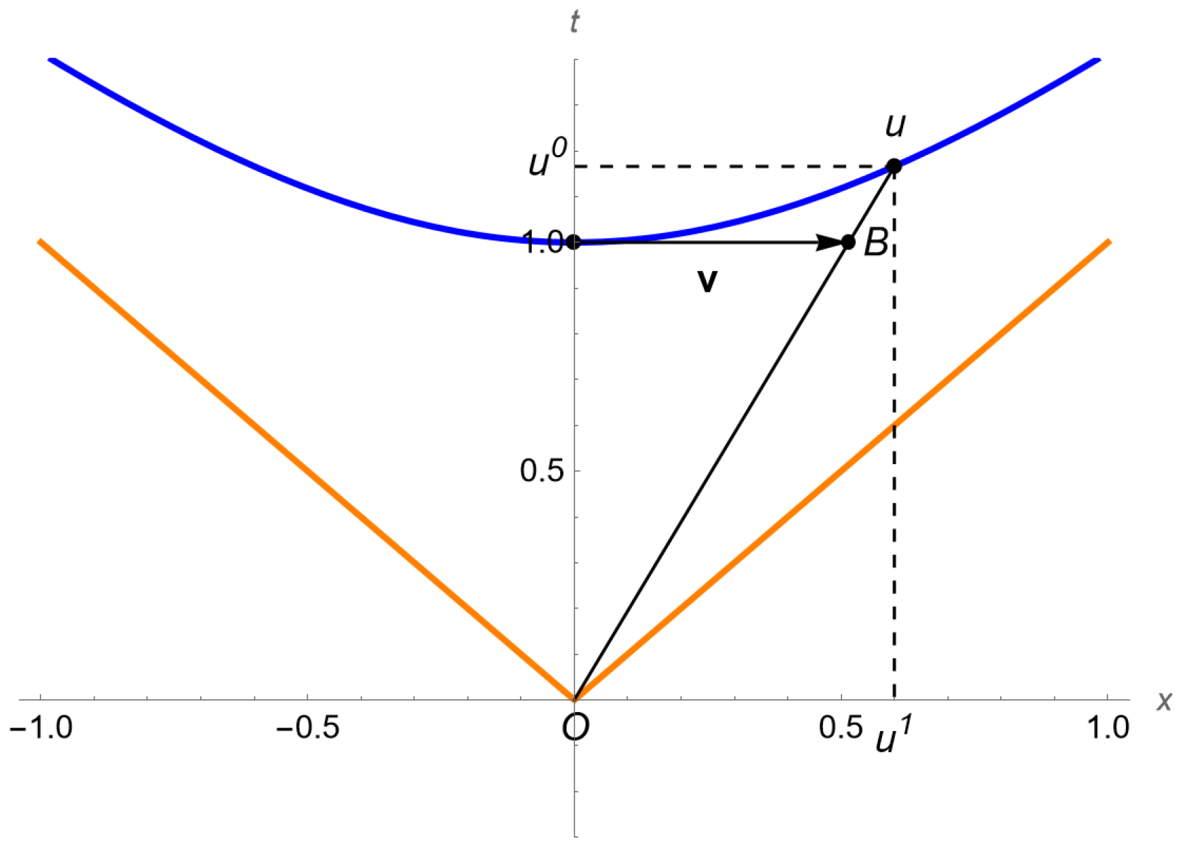
Since the four-velocity has length 1, a Poincaré transformation maps a four-velocity to a four-velocity. See Figure 1 and Figure 2.

Figure 1.
(Orange) A two-dimensional section of the forward light cone with vertex at the origin. (Blue) A two-dimensional section of the hyperboloid of four-velocities. The point B has coordinates , and a multiple of the vector ends at the four-velocity .
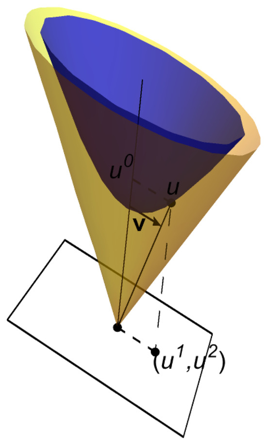
Figure 2.
(Beige) A three-dimensional section of the forward light cone . (Blue) A three-dimensional section of the hyperboloid of four-velocities. As in Figure 1, the connection between u and is displayed.
The Lorentz transformations can be used to derive the Einstein velocity addition, which should, in fact, be called the Einstein velocity composition. It is defined in the following way. Let K and be two inertial frames, where has velocity in K. Suppose an object has velocity in . Then, the velocity of this object in K is denoted by .
The velocity ball is the set of all 3D relativistically admissible velocities:
is a bounded symmetric domain with respect to the automorphism group of affine transformations; see [14].
Instead of viewing a frame as having velocity in K, one can see the two frames as moving away from a central point in opposite directions with the symmetric velocity, where . The ball of relativistically admissible symmetric velocities is a bounded symmetric domain with respect to the automorphism group of conformal transformations. The automorphisms of belong to the real part of a spin- representation of the Lorentz group. In this paper, we will not explore conformal geometry.
4. Lorentz Covariance
The Principle of Relativity requires that our local scaling functions be Lorentz covariant. To formalize this requirement, we now define Lorentz covariance explicitly.
Consider a worldline in an inertial frame K. Let be another inertial frame, and let M and denote the sets of spacetime positions in K and , respectively. The Poincaré transformation maps spacetime points in K to those in , and the same worldline in is given by . Now, let be a four-vector-valued function that depends on . We say that the function is Lorentz covariant if, for any spacetime position x in K, the Poincaré transformation maps to the same four-vector as maps .
Visually, this condition is captured by the commutativity of the following diagram:
This means that satisfies the Lorentz covariance condition, expressed as follows:
for all and all Poincaré transformations on M.
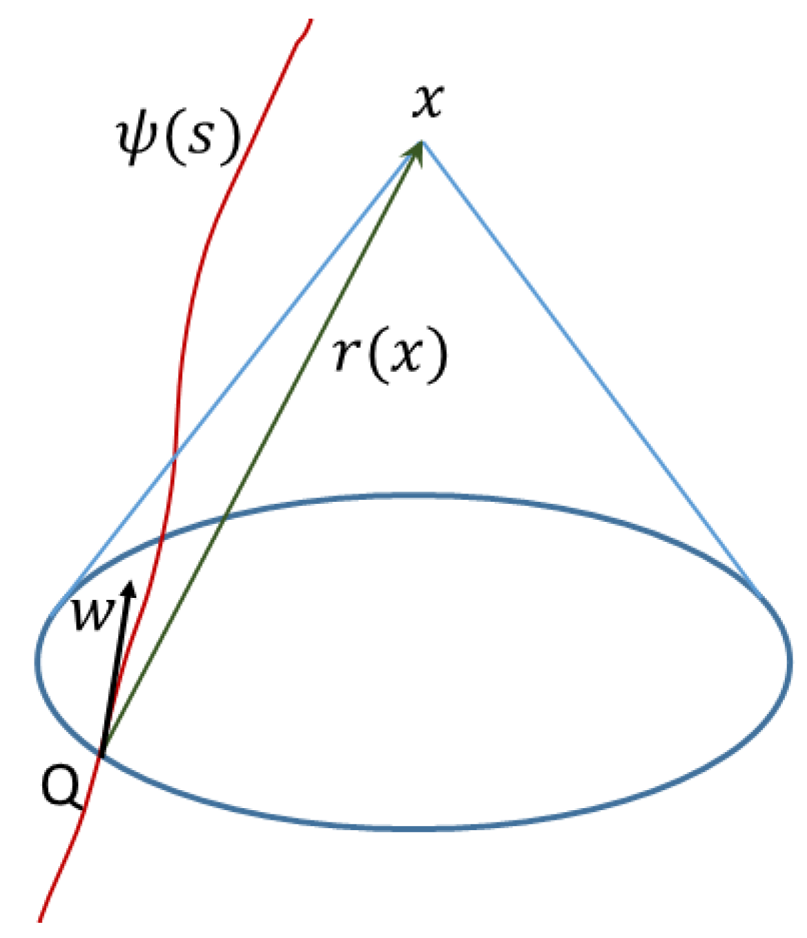
Consider a field (gravitational or electromagnetic) generated by a single source with worldline (Figure 3). Let x be an arbitrary spacetime point. The retarded time is defined by the conditions
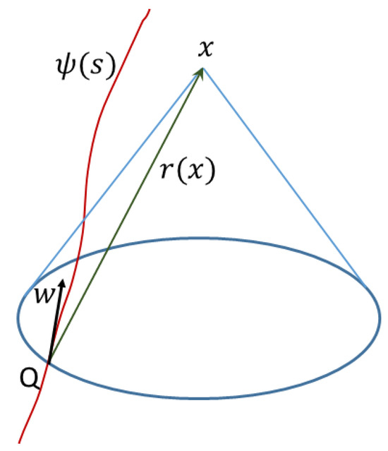
Figure 3.
The point called the retarded position, is the unique intersection of the backward light cone , with a vertex at x and the worldline of the source. is the retarded time and is the four-velocity of the source at the retarded time.
The point Q with coordinates is the unique intersection of the source’s worldline and the backward light cone with vertex x, i.e.,
Since the field propagates at the speed of light, the source’s position at the retarded time fully determines the field at x. The relative position four-vector
represents the displacement from the source at the retarded time to the field point x. This defines a four-vector-valued function that depends on the source’s worldline .
We now verify that the four-vector-valued function is Lorentz covariant. Let be a Poincaré transformation, and define and . Using Equation (9), we obtain
Thus, we conclude that .
Since is a four-vector, Equation (3) implies that acts linearly on . Therefore, we find
This confirms that Equation (11) holds, meaning that is Lorentz covariant.
Beyond the four-vector , the four-velocity of the source at the retarded time is also a Lorentz-covariant four-vector-valued function.
Moreover, the inner product is a Lorentz-invariant scalar, as is any scalar function of . As an example, we define the conjugation ∗w of with respect to the four-velocity as
The four-vector-valued function is Lorentz covariant. It can be directly verified that and that this conjugation reverses the spatial direction of in the frame moving with four-velocity w, while leaving the time component unchanged.
At each point x, the most general form of a Lorentz-covariant four-vector-valued function is given by
where g and h are scalar functions of the Lorentz-invariant scalar .
Later, we will require the first-order derivatives of the relative position null four-vector , the four-velocity of the source, and their inner product . Following [15], the partial derivative of , denoted by , is given by
The derivatives of the source four-velocity are
where is the four-acceleration covector of the source at the retarded time. Similarly, the derivative of is
5. The Relativity of Spacetime Geometry and the Extended Principle of Inertia
In General Relativity (), as previously mentioned, a massive object curves spacetime in the same way for all objects. This curved spacetime acts as a universal stage on which all objects move. The principle underlying this idea was first proposed and tested by Galileo four centuries ago and was reconfirmed on the Moon in 1971, when a hammer and a feather fell to the surface at the same rate. This demonstrates that gravity is independent of an object’s properties, making it naturally suited for a geometric description. Indeed, was the first realization of Riemann’s profound idea that “force equals geometry”.
We now seek to extend geometric concepts to electromagnetic (EM) fields. However, unlike gravity, the electromagnetic force depends on an intrinsic property of the object experiencing it – its charge-to-mass ratio. Consider a fixed positive charge Q and three nearby test particles as follows: one positive, one negative, and one neutral. The positive charge is repelled and accelerates away from Q, the negative charge is attracted and accelerates toward it, while the neutral particle, unaffected by Q, moves uniformly. This demonstrates that the electromagnetic field does not provide a universal geometric framework for all particles. Even among charged particles, no single geometry applies, as acceleration depends on the charge-to-mass ratio. Unlike gravity, electromagnetism is inherently object dependent.
A similar principle governs the propagation of light in a medium. As shown in Figure 4, a prism disperses white light into its constituent colors. According to Snell’s law, the angle of refraction depends not only on the incident angle and the speed of light in the medium (typically less than c) but also on the frequency of each photon. Photons with different frequencies are refracted at different angles, revealing that the trajectory of a photon is determined by an intrinsic property—its frequency. Just as charged particles in an electromagnetic field follow different paths based on their charge-to-mass ratio, photons in a medium follow object-dependent trajectories.
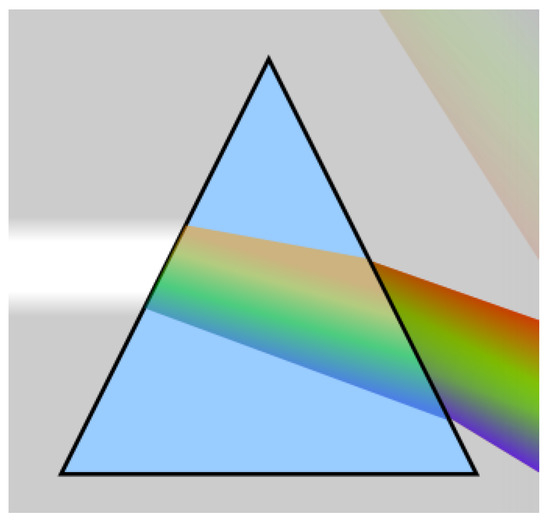
Figure 4.
Relativity of light propagation. A prism disperses white light into its constituent colors, illustrating that photons of different frequencies have different spacetime geometries. Used with permission from Creative Commons under the license https://creativecommons.org/licenses/by-sa/3.0/deed.en (accessed on 10 August 2022). The original image was cropped.
These examples raise the following fundamental question: Can Riemann’s principle that “force equals geometry” be extended to object-dependent forces? If a force does not establish a common stage for all objects, how can a geometric description even begin? This chapter addresses this challenge by introducing the following two key concepts: the relativity of spacetime geometry and the Extended Principle of Inertia.
The relativity of spacetime geometry asserts that spacetime geometry is not universal, but object dependent—each object experiences its own spacetime geometry. For instance, a positive charge moves in a spacetime geometry different from that of a negative charge, and red light follows a different trajectory from that of blue light.
What determines an object’s spacetime geometry? It is shaped by the forces acting on the object and, at most, one intrinsic parameter. For a neutral mass, only gravity defines its geometry—its mass plays no role. A charged particle, however, is influenced by both gravity and electromagnetism, so its spacetime geometry depends on source masses, source charges, and its own charge-to-mass ratio. Similarly, a photon’s motion in a medium depends on the medium’s properties and, at most, one intrinsic characteristic of the photon—its frequency.
How does an object move in its own spacetime? The answer lies in an extension of the Principle of Inertia. The Principle of Inertia states that an object in free motion follows a straight worldline in Minkowski space. When forces are present, its trajectory appears curved. Before Riemann, the prevailing explanation for the curvature was that forces actively bend an object’s worldline. Riemann, however, proposed a different perspective, outlined as follows: forces modify the geometry of spacetime itself. In this new geometry, the object’s trajectory remains “straight”—but in a generalized sense—it follows a geodesic, the natural straight-line path in curved spacetime.
Motion along a geodesic corresponds to motion at constant velocity. An object maintains constant velocity because it has no internal mechanism, like an engine or steering system, to alter its motion. This is evident in the absence of external forces. However, even when forces are present, the object still cannot actively change its velocity. Rather, it continues along a geodesic, following a “straight” or stationary worldline in its own spacetime.
Einstein adopted this idea in :mass curves spacetime, and objects move along geodesics in this curved spacetime. To an inertial observer, an object’s trajectory appears curved, but in the object’s own spacetime, it follows a “straight” geodesic.
Our goal is to extend this reasoning beyond gravity to electromagnetism and motion in media. However, since non-gravitational forces do not act universally, we cannot assume a priori that spacetime curvature is independent of the moving object. Instead, we allow the object’s spacetime geometry to depend on, at most, one intrinsic property of the object.
These ideas lead to the Extended Principle of Inertia:
Since an inanimate object (undisturbed by external contact) cannot change its velocity of its own accord, its worldline remains stationary in its own spacetime.
This principle implies that every object moves along a geodesic in its own spacetime geometry. (By “undisturbed”, we mean the absence of direct contact forces such as collisions.)
To compute geodesics, we need a method to measure worldline lengths in an object’s spacetime. For this, we introduce local scaling functions. Applying the Euler–Lagrange equations to the local scaling function of a geometry produces the equation of motion, or geodesic equation, for this geometry.
6. The Local Scaling Function and Its Properties
We now determine the properties that a local scaling function must have in order to describe relativistic dynamics.
The first step is to work in an inertial frame in Minkowski space, rather than a non-inertial frame in the object’s own spacetime. Performing calculations in an inertial frame significantly simplifies the model. This approach is analogous to measuring geographic distances on a flat map rather than directly on the curved surface of a globe.
To determine the shortest worldline, we first need a precise definition of length in an object’s spacetime. This requires defining the distance between two infinitesimally close points, P and Q, in the object’s spacetime—analogous to the line element in the spacetime metric of [16,17,18]. We propose the following definition.
Definition 1.
The local scaling function is a scalar-valued function of a spacetime position x and a four-vector u, with the meaning that the infinitesimal distance between two points and in an object’s spacetime is if ϵ is small.
Mathematically, the local scaling function , where denotes the distance in the object’s spacetime between two spacetime points x and y.
We now provide some examples of local scaling functions.
Example 1.
Finding the shortest route to the top of a hill.
We consider a flat map representing a hill, where the scale is 1 mm = 100 m. Although the map itself is flat, it depicts points at different altitudes. When projecting real-world points onto the map, we lose information about elevation. For example, two points at the base of the hill that are 100 m apart correspond to 1 mm on the flat map. However, near the hill’s peak, two points that are 1 mm apart on the map may not be exactly 100 m in reality. The actual distance depends on the slope of the hill in the direction being measured. The local scaling function accounts for this variation. It provides a way to adjust the 1 mm distance on the flat map to reflect the true distance on the hill, in any given direction. Using this function, we can accurately measure the length of a road along the hill and determine the shortest route to the top. Notably, the distance between two points x and y on the hill is symmetric—meaning the distance from x to y is the same as the distance from y to x.
Example 2.
Finding the route to the top of the hill and back to the bottom which minimizes fuel consumption.
We consider the same hill, but now the local scaling function does not measure physical distances. It measures how much fuel it takes to move from an arbitrary point on the hill in an arbitrary direction. In this case, the fuel consumption from point x to point y is not the same as the fuel consumption from y to x. Going uphill requires energy, while one gains energy going downhill. Later, in Section 9, we will see that the local scaling function for a gravitational field is not the same in opposite directions.
Example 3.
The local scaling function for the Earth.
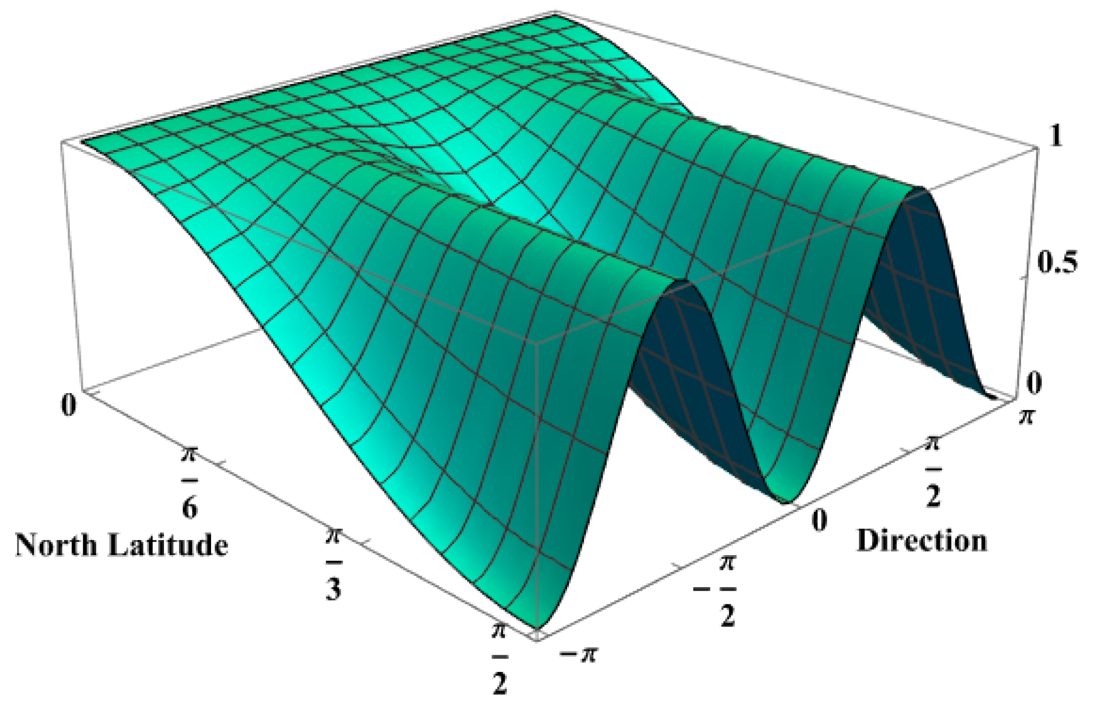
Let be the point on the globe with latitude and longitude . Let be an arbitrary direction from x. Then, the local scaling function for distances on the globe is
where R is the radius of the Earth. Note that the scaling does not depend on the longitude . See Figure 5, where we show the dependence of L on the latitude and the direction .

Figure 5.
The local scaling function for the Earth (with radius 1) is given by The north latitude ranges from 0 to , and the direction from a given point on the globe is represented by an angle , for , where is due east. At the equator (), L remains constant at 1 because infinitesimal distances are the same in all directions. Similarly, when , since distances in the north–south direction are identical for all values of . However, when or , the heading is due east or due west. As increases from 0, each degree of longitude corresponds to a progressively smaller physical distance due to the curvature of the Earth.
By definition, the length of a worldline appears to depend on its parameterization . However, we require that the length remains independent of the chosen parameterization. This ensures flexibility, allowing us to select different parameters for different problems—an approach that can significantly simplify calculations. To achieve this, we now derive a sufficient condition that guarantees the desired parameter independence.
Let be another parameterization of the same worldline. Define a function such that . Since parameterizations must preserve order, the derivative . Now and , implying that
Thus, in order to have , we need
In other words, for any positive scalar a, we require that . This means that must be positive homogeneous inu of degree 1.
In light of Definition 1, the Principle of Relativity, and the above considerations, the local scaling function must satisfy the following properties:
- P1
- In order to satisfy the Principle of Relativity, must be a Lorentz-invariant scalar.
- P2
- must be positive homogeneous in u of degree one so that the length will not depend on the choice of parameter .
- P3
- When the strength of the field goes to zero, the local scaling function should approach the local scaling function of Minkowski space.
- P4
- Since the acceleration of a charge in an EM field depends only on its charge-to-mass ratio , and the motion of a photon in a medium depends only on its frequency, must depend on, at most, one parameter intrinsic to the object.
In the next section, we construct a local scaling function with all of these properties.
To finish this section, we briefly review the Euler–Lagrange equations. Let be a function of eight variables , for , where x is a spacetime position and u is a four-vector.
For an arbitrary worldline , we define the length of the worldline to be
The worldline is called stationary if
for any smooth satisfying .
For each , we define the unit-free energy–momentum covector associated with as
Theorem 1.
The worldline is stationary if and only if for every μ, we have
Equation (22) is known as the Euler–Lagrange equation. The notation in (21) and (22) means that one first differentiates L by or and then substitutes for x and for u.
We call for the force vector (the minus results from raising the index) and the momentum vector imparted to the object by the field.
Corollary 1
(The Law of Conservation). If the function does not depend on , then the μ component of the energy–momentum covector, defined by (21), is conserved along stationary worldlines. That is,
7. Simple Local Scaling Function
We seek the simplest function that satisfies the above properties. This approach aligns with Occam’s razor, which states the following: “Explanations that posit fewer entities, or fewer kinds of entities, are to be preferred to explanations that posit more”. Einstein echoed this principle, famously stating: “A physical theory should be as simple as possible, but not simpler”.
A straightforward way to construct a Lorentz-invariant scalar-valued function of a four-vector u is to contract m copies of with a Lorentz-covariant tensor of rank m.
For , the function takes the form , where is a Lorentz-covariant covector-valued function. For , we obtain , where is a Lorentz-covariant rank 2 tensor. Notably, we can assume is symmetric since any antisymmetric component vanishes upon contraction with two identical vectors. If necessary, we can symmetrize it via For a higher m, similar contractions with higher-rank tensors apply.
Importantly, any scalar-valued function of these basic Lorentz-invariant scalar-valued expressions remains Lorentz invariant. By using only functions of this type, we ensure Lorentz invariance (P1).
For P2, observe that which demonstrates positive homogeneity of degree 2. However, is homogeneous of degree 1. More generally, any linear combination of terms such as and is both Lorentz invariant and positively homogeneous of degree 1. For P3, must contain a term of at least second order in u.
From Definition 1 of the local scaling function, we know that depends on u in an infinitesimal manner. This suggests that a low-order approximation is sufficient for its definition. Therefore, for simplicity, we assume that consists only of terms up to second order.
This leads us to the following simple local scaling function for an object’s spacetime:
for some constant k, which may depend on the object. This function depends on a Lorentz-covariant metric and on a Lorentz-covariant four-covector Note that if or , meaning either that the object is electrically neutral or that there are no EM fields, then the local scaling function is the square root of the metric of pseudo-Riemannian geometry.
8. The Geometry of the Electromagnetic Field
Consider first the case when the local scaling function (24) is
where is the Minkowski metric . As shown in [7,8], the Euler–Lagrange equations yield the equation of motion in the field as follows:
where
This equation describes the motion of a particle with charge-to-mass ratio in an electromagnetic field characterized by the antisymmetric field strength tensor (see also [15], Equation (12.3)) and the four-potential A. Thus, the local scaling function (25), defined by the four-covector-valued function , known as the electromagnetic potential, governs how an electromagnetic field influences the geometry of an object’s spacetime.
How can we define the electromagnetic field potential for an arbitrary electromagnetic field? The sources of any electromagnetic field are a collection of moving charges. Thus, we first have to define the potential of a single source.
Consider the field generated by a single moving source of charge Q. Let denote the worldline of the source. For a given spacetime position x, let denote the position of the source at the retarded time, and let be the four-velocity of the source at the retarded time. As in (27), we define the relative position null four-vector as
Note that and any function of it are Lorentz invariant. Since must be Lorentz covariant, it must be a combination of the two four-vectors with functions of as coefficients (see (13)). Moreover, for small velocities, the acceleration defined by (26) should coincide with the acceleration in classical electrodynamics. From this, we obtain
for any . If , we obtain the well-known the Liénard–Wiechert four-potential of a single-source electromagnetic field. Hence, in the remainder of this section, we will assume that . Thus, the describing the spacetime geometry of a charge q of mass m, influenced by the source Q, is
where are defined by (27).
Using this local scaling function, we compute the field by applying Equations (15) and (16). To simplify the notation, we define the wedge product of the two covectors a and b. The wedge product is a rank-2 antisymmetric tensor, given by
Using the wedge product, we can express the field as
The first term represents the near field, also known as the Coulomb field, which decays at large distances like . The second term corresponds to the far field, which decays like and describes radiation.
Next, we examine the geometry of an object’s spacetime by considering the influence of the field generated by a charge Q, at rest (i.e., ) at the origin, on a charge with a charge-to-mass ratio . Using Equation (25) and the solution for and in (29), the local scaling function , where , is a unit vector in the plane, and u is an arbitrary four-vector, is given by
where . Here, the dependence on x is encapsulated in R, which represents the distance between the source and the test charge. The four-vector u is . See Figure 6.
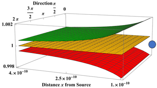
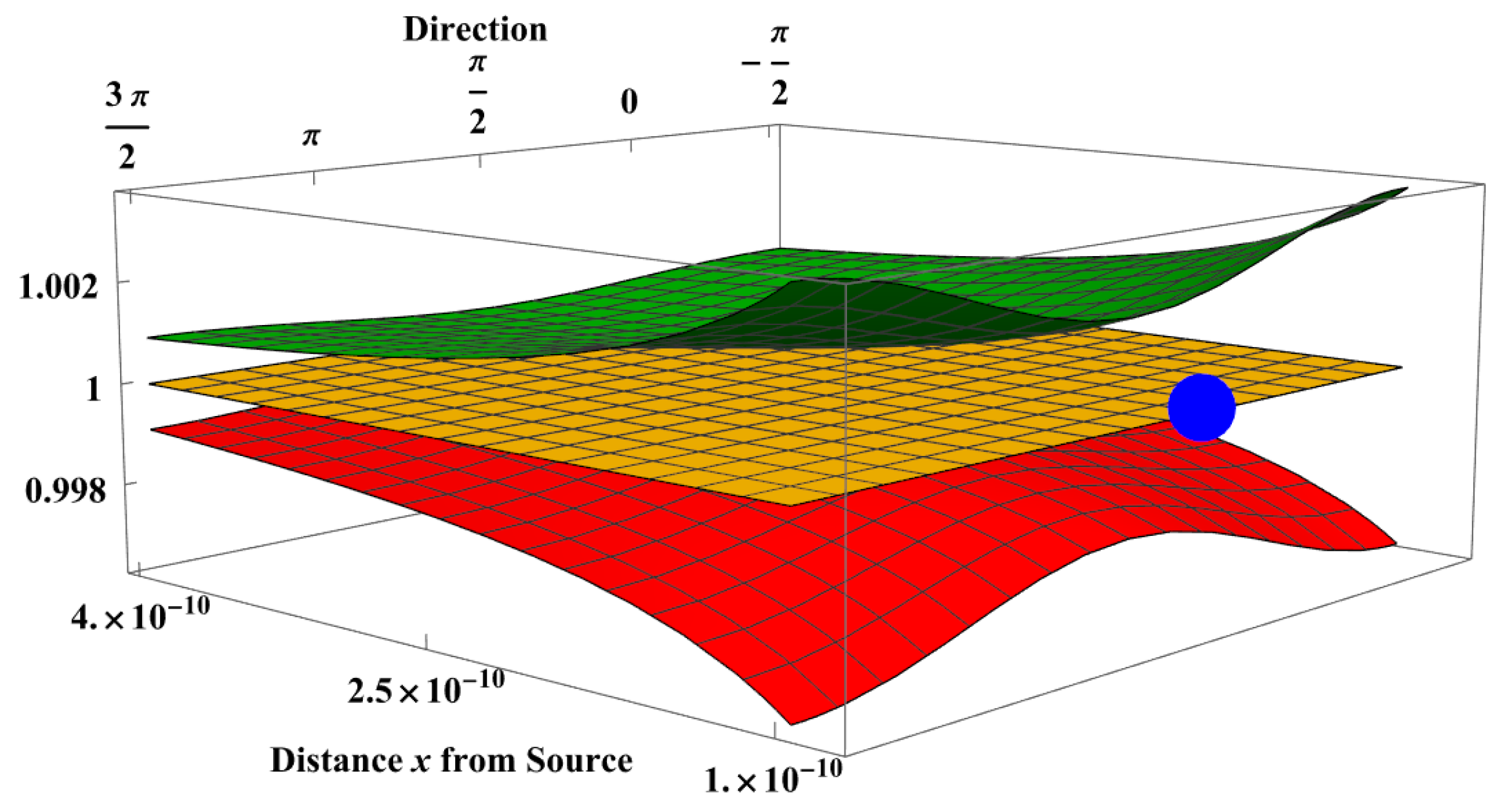
Figure 6.
Local scaling functions for a resting source. The local scaling functions of a field of a positive source Q (represented by a blue dot) at rest at , defined by Equation (32). The green surface is the for a positive test charge, like a positron (, the red one is the for a negative charge, like an electron (, and the yellow one is for a neutral particle (. In all cases, the local scaling function is independent of the spatial direction of u, meaning the momentum imparted by the field is zero. As the test charge moves closer to the source, the force, given by , increases in magnitude. For the positron (), the force is positive, indicating repulsion, while for the electron (), the force is negative, indicating attraction. These results are consistent with the equation of motion (26).
Another way to view the single-source electric field’s geometry, is to compare the EM hyperboloid to the hyperboloid of four-velocities in Minkowski space, see Figure 7.

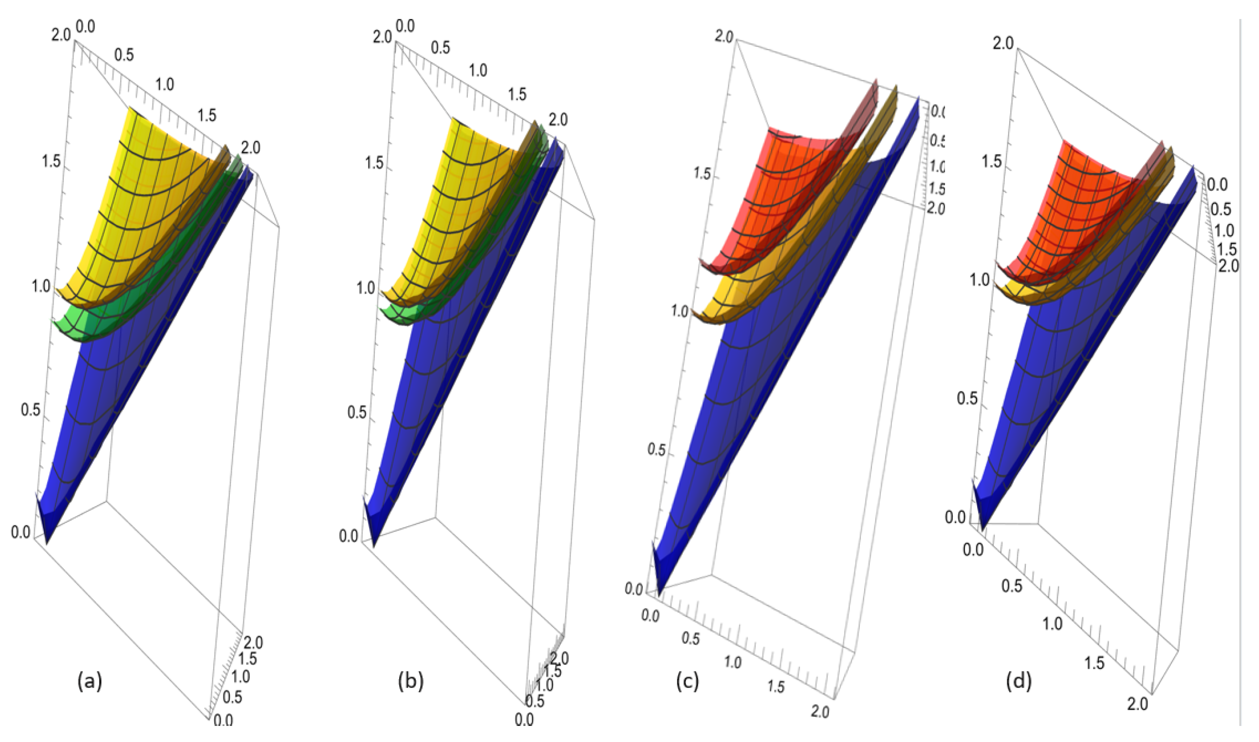
Figure 7.
Influence of an electric field on Minkowski space. The influence of an electric field, generated by a single source charge Q, on Minkowski space is depicted in the following plots. Each plot shows a cutaway view of the upper half of the light cone (blue), the hyperboloid of four-velocities in Minkowski space (yellow), and the electromagnetic (EM) hyperboloid, given by the equation where (green for , red for ). (a,c) correspond to mm, and (b,d) correspond to mm.
In Figure 7, for , the field is repulsive, and the EM hyperboloid
where , lies between the light cone and the four-velocities of Minkowski space, and approaches the four-velocities as the distance from the source increases. For , the field is attractive, and the EM hyperboloid is inside the four-velocities and approaches the four-velocities as the distance from the source increases.
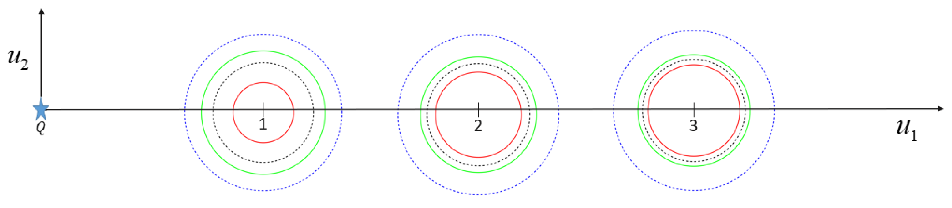
Figure 8 displays horizontal cuts of the light cone, the hyperboloid of four-velocities and EM hyperboloids. Note that all of the cuts are circles and that the EM circles approach the four-velocities as the distance from the source increases.
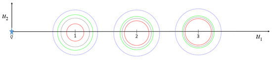
Figure 8.
The influence of a stationary source on the geometry of a test charge with a charge-to-mass ratio is examined at three different distances: and 3 mm. The plot shows the intersection of the plane with the following key geometric structures: the light cone (dashed blue line), the hyperboloid of four-velocities in Minkowski space (dashed black line), and two four-velocity hyperboloids in the electromagnetic field, given by for mm (green solid line) and mm (red solid line). These hyperboloids illustrate how the EM field modifies the spacetime geometry experienced by the test charge at different distances from the source. Nearer the source, the positive EM hyperboloid is pulled away from the four-velocities and towards the light cone, while the negative EM hyperboloid moves away from the four-velocities.
We now explore the spacetime geometry of the field of a moving charge. Suppose a source charge Q is moving with four-velocity at the origin at time . We compute the for a test charge at spatial points for small x. Since the field propagates with the speed of light, and the distances between the source and the test charge are small, we may ignore the retardation and compute the using (29) at in the direction . We have
See Figure 9.

Figure 9.
Local scaling functions for a moving source. The local scaling functions of a field of a positive source Q (represented by a blue dot) moving at velocity in the positive y direction, defined by Equation (33). The green surface is the for a positive test charge, such as a positron (, the red surface is the for a negative charge, such as an electron (, and the yellow plane is the for a neutral particle (. The strength of the electric field is greatest when (or ), which is the direction antiparallel to the velocity of the source. The field is minimal when , which is the direction parallel to the velocity of the source.
Comparing Figure 9 to Figure 6, we observe that for a rest charge field, the is independent of direction , implying that the momentum of the field defined by (21) vanishes, while for a moving charge, the field has a momentum. This field momentum is acquired by the field from the momentum of the source. Moreover, the source’s angular momentum is also transferred to the field, and as shown in [8], is manifested as a magnetic field.
Using the local scaling function (25) and the four-potential (29), and setting and , the local scaling function at a point is
where . Figure 10 displays horizontal sections of EM hyperboloids , with , , , and mm, at different distances from the source’s current position.
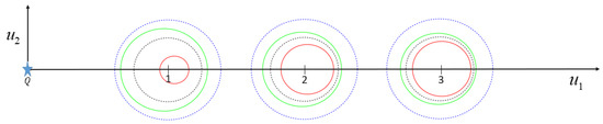
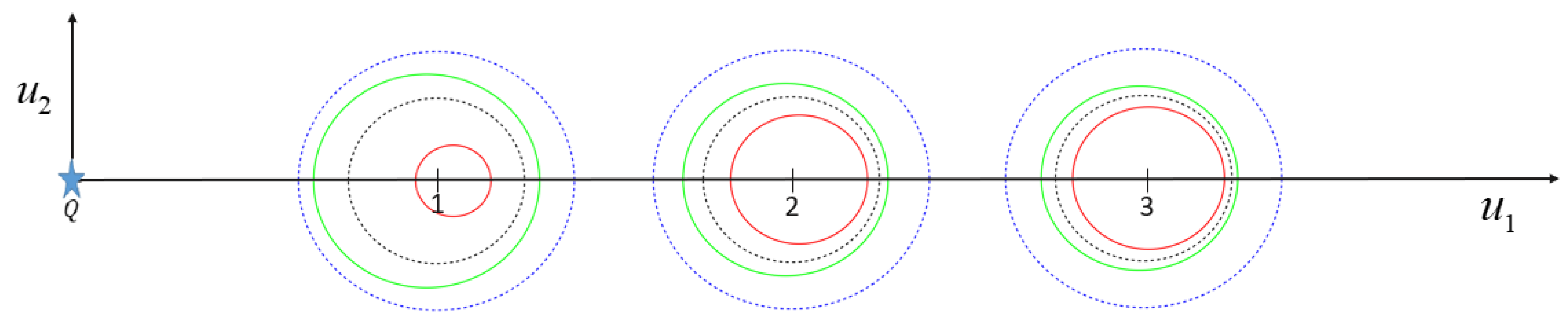
Figure 10.
Effect of a source with four-velocity on the geometry of a test charge with charge-to-mass ratio , at three different distances mm from the source’s current position. Displayed are the intersection of the plane with the light cone (dashed blue line), the hyperboloid of four-velocities in Minkowski space (dashed black line), and the EM hyperboloids , where , and mm (green solid line), and mm (red solid line). For , the four-velocities are shifted in the direction of the velocity of the source. For , the four-velocities are shifted in the opposite direction.
As shown in Figure 8, when the source is at rest, the electromagnetic (EM) sections are circles. However, when the source moves uniformly, the sections become ellipses. For a negatively charged source, the ellipses are shifted in the direction of motion, whereas for a positively charged source, they shift in the opposite direction. As the distance from the source increases, these ellipses approach circular shapes. For more detailed geometry near a test charge, especially when the source is moving near the path of a positive or negative charge, refer to Figure 9.
What are the geodesics in the spacetime of a single source? As shown in [8,19], there are both bounded and unbounded geodesics. The bounded geodesics are precessing ellipses with one focus at the source of the field, while the unbounded geodesics resemble hyperbolas. For a uniformly moving charge, the geodesics can be derived by Lorentz transforming the geodesics from the comoving inertial frame to our lab frame K.
The source of a general electromagnetic field is the flow of moving charges, which we represent in an inertial frame K by a four-current density. This four-vector is given by the following:
where is the volume charge density in K, and is the current density in K.
For a field generated by several sources, we assume that the four-potential is the sum of the individual four-potentials. To define the four-potential for an arbitrary electromagnetic field, we integrate the four-potential from a single source over the backward light cone. In spherical coordinates, the four-potential of such a field is given by the following:
where . The local scaling function () for this field is obtained by substituting this four-potential into the expression for the electromagnetic action (25).
Note that we obtained the relativistic dynamics of charges in an electromagnetic field directly from the sources of the field, without the need for Maxwell’s field equations. As shown in [8], these equations can be derived from our geometric description and conservation of charge.
9. The Geometry of the Gravitational Field
Consider now the local scaling function , defined by (24), with . Thus,
We decompose this metric as
where represents the deviation from the Minkowski metric due to the gravitational field. We call the deviation tensor of the gravitational field.
To compute the geodesic equation for this , we follow [20]. First, we introduce a tensor
and an operator
With this notation, the well-known Christoffel symbols become
The Euler–Lagrange equations then lead to the following equation of motion, with respect to the invariant parameter s:
For a single-source field, we assume that the deviation tensor is proportional to the mass M of the source and that there is a four-potential such that
where
is the Schwarzschild radius. Under these assumptions, the local scaling function is
Using (27), we define the Lorentz-covariant relative position null four-vector and the four-velocity of the source at the retarded time. Since is required to be Lorentz covariant, it follows from (13) that it is a combination of the two four-vectors r and w, with functions of as coefficients. Moreover, at low velocities, the acceleration defined by (42) should coincide with the acceleration predicted by Newtonian gravity. From this, we obtain
where is defined by (12). This is the gravitational analog of the Liénard–Wiechert four-potential of a moving charge.
Consider now the gravitational field of a massive object resting at the origin. In this case, and , where is a norm-one 3D spatial vector. This implies that . It follows from (46) that for this field, we have . Thus, letting , the is
As shown in [8], the dynamics resulting from (42) for the geometry defined by (47) passes all the classical tests of . The model predicts the correct precession of the perihelion of Mercury, the correct periastron advance of a binary star, and orbits in the strong-field regime. For massless particles, the model predicts the known formulas for gravitational lensing and the Shapiro time delay.
To understand the change in geometry due to a single-source gravitation field, we observe that the local scaling function (45) of a gravitational field is defined only when the expression under the square root is non-negative. Thus, the admissible four-velocities in a single-source gravitational field belong to the domain
The velocity of light (or any massless particle) belongs to the boundary
of , where .
One way to visualize the geometry of the spacetime influenced by a gravitational field is to draw the boundary at various spatial positions in the field. We decompose the velocity of a light ray in the field into radial and transverse components , where is a unit vector perpendicular to . Then the four-velocity is
and . Denoting and using the definition (49) of the boundary, we obtain
or
For example, if the velocity of a massless particle at x is transverse, then
Equation (51) defines an ellipse in of admissible velocities of light. Direct substitution shows that satisfies this equation. This means that in the direction towards the source, the speed of light is c, which is the speed of light in vacuum. Another solution is , which means that in the direction away from the source, the speed of light is slowed by the factor . This implies that at the Schwarzschild radius, where , the speed of light becomes 0, showing that even light cannot escape the region inside the Schwarzschild radius. Sometimes, the source of the field is extremely compact and entirely inside its Schwarzschild radius. In this case, we call the source a black hole. Figure 11 displays the admissible velocities at different distances from a black hole.
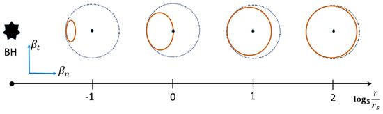
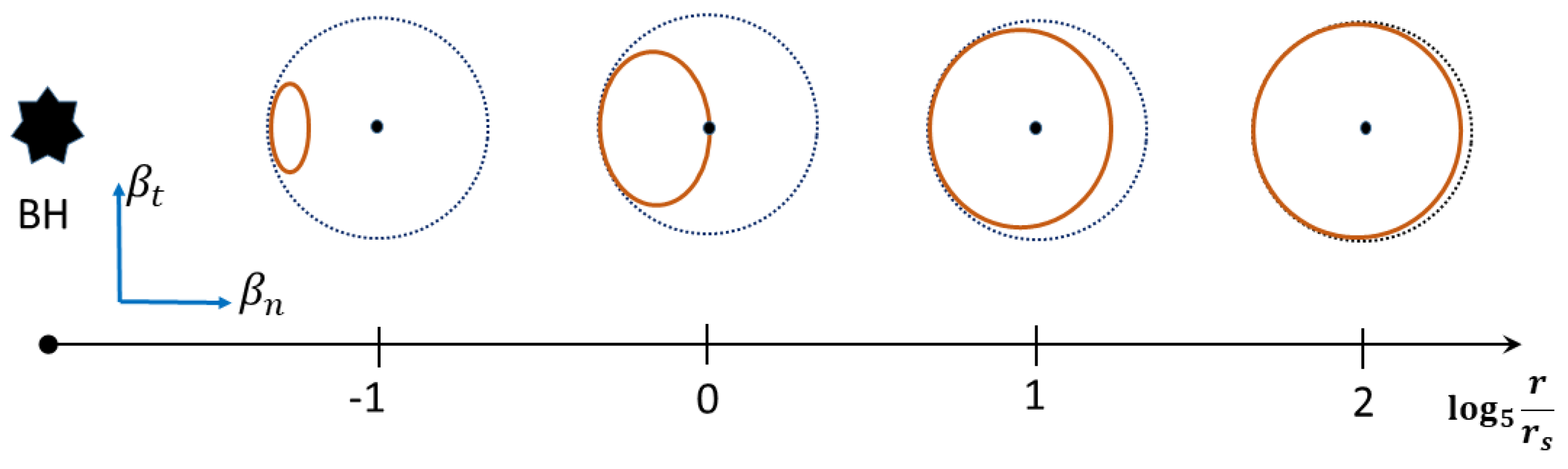
Figure 11.
The ball of admissible velocities in the vicinity of a black hole (BH) is depicted. The figure illustrates a 2D cross-section of the ball in both Minkowski space (blue, dotted) and the curved spacetime influenced by the black hole (brown, solid) at various distances from the BH: , where is the Schwarzschild radius. As the distance decreases, the BH pulls the ball towards itself, indicating the bending of light paths. Below the Schwarzschild radius, light is unable to escape, marking the event horizon as a boundary beyond which no information can reach an outside observer.
Another way to view the geometry of the gravitational field is to draw cross-sections of the . In Figure 12, we see the defined by (47), where the distance from the black hole ranges from to , and , with .
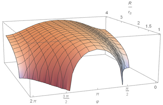
Figure 12.
The local scaling function (47) near a black hole with , , and . As R increases, the function’s behavior resembles that of a moving electromagnetic source in the attractive case, indicating that a gravitational field imparts momentum to objects even when the source is stationary (compare to Figure 9). In this range, motion is possible in all directions. Closer to the Schwarzschild radius, permissible motion directions become increasingly constrained, with outward movement becoming impossible at the Schwarzschild radius.
In order to compute the equation of motion (42) explicitly for a single-source gravitational field, we need to compute the tensor G, defined by (39), and the operator H, defined by (40). The operator H is defined from the deviation tensor given by (43) and (46). To define the tensor G, we need the partial derivatives of both the relative position r and the retarded four-velocity w. These are given in (14)–(16). After these calculations, we discover that, just as in the electromagnetic field, the gravitational field has both near and far components.
Consider now the gravitational field generated by several spherically symmetric moving sources. For source k, the relative position is denoted by , the retarded four-velocity is , and the Schwarzschild radius is . Calculate the four-potential and the deviation using formulas (46) and (43) for each source k. Since the deviation is linear in the mass of the source, we may assume, as in [21], that the deviation of the combined field from the Minkowski metric is
The metric of the combined field is
Using these formulas, one can describe gravitational waves.
10. Propagation of Light in Media
We analyze the propagation of light in an isotropic medium at rest. Each photon moves in a spacetime influenced by the medium. Since the photon’s charge q is zero, the parameter in the simple local scaling function defined by (24). Consequently, the local scaling function for photon propagation in an isotropic medium is given by
Because the medium is isotropic and at rest, the deviation tensor is independent of the spatial directions. Thus, the spatial components of must vanish, and we assume that only is nonzero and depends on the properties of the medium. Additionally, it may also depend on the photon’s frequency, as frequency is the only intrinsic property distinguishing photons. This leads to a of the form
If we choose the time t as the parameter along the photon’s worldline, the four-velocity is given by , where is the photon’s 3D velocity in the medium. Since must vanish for a photon, its velocity satisfies . It is well known that the speed of light in a medium is always less than the speed of light in a vacuum and may vary with frequency. The refractive index n of a medium is defined as . Substituting this into (56), we obtain the
This result implies that the geometry of the photon’s spacetime in a medium at rest is equivalent to the geometry of empty space, but with the vacuum speed of light c replaced by , the speed of light in the medium.
Until this point, we have considered the motion of a photon only in media at rest. The for a moving medium may be obtained by Lorentz transforming the rest from the frame comoving to the medium to our lab frame. We may thus obtain the speed of light in moving media. These results agree with the observed velocities of light in moving water in the Fizeau experiment.
We now consider the refraction of a light ray propagating between two media separated by a planar interface, which we take to be the plane. Let and be the refractive indices of the upper () and lower () media, respectively. The x-axis is chosen such that the incident ray lies in the plane .
Thus, the ratio of spatial to temporal momentum components simplifies to
For our problem, the local scaling function depends on through but is independent of and . Consequently, from (23), we conclude that along a stationary worldline, the ratio is conserved.
It is important to note that and are not defined on a photon’s worldline because there, leading to divergences in these quantities. However, certain ratios remain well defined when evaluated along worldlines that approach the photon’s trajectory. The limiting values of these ratios are finite and thus meaningful on the photon’s worldline.
Since the photon’s worldline is stationary, choosing as the parameter, we find
For the upper medium, the x-component of velocity is , where is the angle of incidence. Substituting this into the ratio equation gives
Similarly, in the lower medium, we obtain
Since is conserved along a stationary worldline, it follows that
This is precisely Snell’s law for light refraction.
Conclusion: The refraction of light is a direct consequence of the conservation of the ratio of a photon’s momenta. This conservation law elegantly explains why light bends when transitioning between media of different refractive indices.
11. Summary and Discussion
In this paper, we implement Riemann’s idea that “force equals geometry”. This principle suggests that a force acting at a distance alters the geometry of spacetime and that the motion of an object is dictated by these geometric changes. The connection between free motion and straight-line trajectories in spacetime naturally follows from Galileo’s Law of Inertia.
We analyze the motion of point-like objects under the influence of electromagnetic and gravitational fields and examine the propagation of light in media. Each of these motions is represented by a worldline in Minkowski space M. The Principle of Relativity implies that the laws governing motion must be Lorentz covariant under an appropriate representation of the Poincaré group on M.
To describe how spacetime geometry is influenced by external fields and media, we introduce a local scaling function , an extension of the concept of metric, but allowing for linear as well as quadratic dependence of displacements. This function defines the scale between the distances in M and the corresponding distances in the influenced spacetime between two nearby points x and . The worldline of motion is then a geodesic with respect to , determined by the Euler–Lagrange equation.
The structure of the paper is as follows:
- •
- Section 3: Review of the fundamental properties of Minkowski space geometry.
- •
- Section 4: Construction of Lorentz-covariant vectors and functions for geometries.
- •
- Section 5: Introduction of the Extended Principle of Inertia and the relativity of spacetime geometry, which are two new ideas that are essential for generalizing Riemann’s idea to electromagnetism and optics.
- •
- Section 6: Defining the local scaling function and tailoring it to physical laws. We also recall the Euler–Lagrange Theorem, which governs geodesic motion.
- •
- •
- Section 8: The spacetime geometry of an electromagnetic field. The geometry of an electromagnetic field is determined by the electromagnetic potential (26). Geodesic motion in this geometry coincides exactly with classical electrodynamics. First, we define the potential for a single-source field, using the local scaling function (29). We then generalize to arbitrary electromagnetic fields via Equation (36), but without the need for Maxwell’s equations. We provide visualizations of the geometry via graphs and cross-sections of the local scaling functions and the EM hyperboloids of four-velocities. We observe that an EM source at rest imparts no momentum to the field, but if the source is moving, then its momentum is transferred to the field. Moreover, the transfer of its angular momentum produces a magnetic field.
- •
- Section 9: The spacetime geometry of a gravitational field. We first consider a single-source gravitational field, described by the local scaling function (45), with the four-potential defined in (46). The geometric changes near a black hole are discussed and displayed visually. Using our new superposition principle for gravity, we obtain the local scaling function for a general gravitational field (53) and (54), without the need for field equations.
- •
- Section 10: Light propagation in isotropic media. We define the local scaling function for a photon in the medium. We show that Snell’s law of refraction is an expression of the conservation of the ratios of the photon’s momenta.
11.1. Results
The geometric framework of General Relativity () is based on pseudo-Riemannian geometry, where the metric is non-positive definite. However, this formalism is not directly applicable to electromagnetism, as electromagnetic interactions depend linearly on displacements rather than quadratically. Furthermore, operates on a curved manifold, which, while powerful, often complicates calculations.
We have demonstrated that all known relativistic gravitational effects can be reproduced while working entirely within Minkowski space coordinates. By defining a new metric for a single gravitational source, we extended this approach to describe the geometry of a field generated by multiple sources. Unlike , where the gravitational field is determined by Einstein’s nonlinear field equations, our model derives the metric from a superposition principle.
This unified framework seamlessly incorporates gravity, electromagnetism, and optics under the same fundamental principles. While the superposition principle is well established in electromagnetism, no such principle has existed for gravity—until now. The gravitational superposition principle we propose enables analytical solutions for problems that cannot handle directly. In particular, we have obtained exact solutions for the metric of an extended, spherically symmetric body and the equations of motion within such a field.
A key tool in our approach is the local scaling function, which plays a role analogous to the metric. It provides an intuitive way to visualize geometry by illustrating how the ball of admissible velocities is influenced by external fields. Additionally, by examining different cross-sections of the local scaling function, we can extract valuable insights regarding the properties of fields generated by different sources.
11.2. Future Directions
This approach opens new possibilities for research. In the case of electromagnetic fields:
- •
- It would be interesting to determine the geodesics for the field generated by a uniformly accelerating charge.
- •
- We need to investigate the implications of in Equation (28).
- •
- Do there exist fields for which ?
- •
- Are there accelerating sources that do not radiate?
For gravitational fields, our methodology provides a way to derive relativistic corrections for extended (not point-like) gravitational sources and galactic motion.
In this paper, we have focused on the relativistic dynamics of point-like objects. However, as shown in [8], extended objects require complexifying Minkowski space to incorporate spin effects. Physically, this also necessitates the transition to a spin- representation of the Lorentz group. We plan to continue this line of research. Some preliminary results can be found in [8].
Author Contributions
Conceptualization, Y.F.; methodology, Y.F.; software, T.S.; validation, Y.F. and T.S.; writing—original draft preparation, Y.F. and T.S.; writing—review and editing, Y.F. and T.S.; visualization, Y.F. and T.S.; supervision, Y.F. All authors have read and agreed to the published version of the manuscript.
Funding
This research did not received any external funding.
Data Availability Statement
Data are contained within the article.
Conflicts of Interest
The authors declare no conflict of interest.
Abbreviations
The following abbreviations are used in this manuscript:
| Local Scaling Function | |
| General Relativity |
References
- Lochak, G. La Géométrisation de la Physique; Flammarion: Paris, France, 1994. [Google Scholar]
- Klein, F. Riemann and their significance for the development of modern mathematics. Bull. Am. Math. Soc. 1895, 1, 165–180. [Google Scholar] [CrossRef]
- Papadopoulos, A. Physics in Riemann’s Mathematical Papers. In From Riemann to Differential Geometry and Relativity; Ji, L., Papadopoulos, A., Yamada, S., Eds.; Springer: Cham, Switzerland, 2017; pp. 151–207. [Google Scholar]
- Minkowski, H. Raum und Zeit (Space and Time). Phys. Z 1908–1909, 10, 75–88. [Google Scholar]
- Einstein, A. Ideas and Opinions; Seeling, C., Ed.; Bargmann, S., Translators; Crown Pub.: New York, NY, USA, 1954. [Google Scholar]
- Duarte, C. The classical geometrization of the electromagnetism. Int. J. Geom. Methods Mod. Phys. 2015, 12, 1560022. [Google Scholar] [CrossRef]
- Friedman, Y. A unifying physically meaningful relativistic action. Sci. Rep. 2022, 12, 10843. [Google Scholar] [CrossRef] [PubMed]
- Friedman, Y.; Scarr, T. A Novel Approach to Relativistic Dynamics: Integrating Gravity, Electromagnetism and Optics; Fundamental Theories of Physics; Springer Nature: Cham, Switzerland, 2023; Volume 210. [Google Scholar]
- Romero, C.; Fonseca-Neto, J.; Pucheu, M. General relativity and weyl geometry. Class. Quantum Gravity 2012, 29, 155015. [Google Scholar] [CrossRef]
- Goto, S.; Hino, H. Expectation Variables on a Para-Contact Metric Manifold Exactly Derived from Master Equations. In Geometric Science of Information; Springer: Cham, Switzerland, 2019. [Google Scholar] [CrossRef]
- Riley, K.F.; Hobson, M.P.; Bence, S.J. Mathematical Methods for Physics and Engineering, 3rd ed.; Cambridge University Press: New York, NY, USA, 2006; p. 787. [Google Scholar]
- Einstein, A. Zur Elektrodynamik bewegter Körper. Ann. Phys. 1905, 17, 891. [Google Scholar] [CrossRef]
- Einstein, A. The Meaning of Relativity; Princeton University Press: Princeton, NJ, USA, 1955. [Google Scholar]
- Friedman, Y. Physical Applications of Homogeneous Balls. In Progress in Mathematical Physics; Birkhauser: Boston, MA, USA, 2004; Volume 40. [Google Scholar]
- Jackson, J.D. Classical Electrodynamics, 3rd ed.; John Wiley & Sons.: Hoboken, NJ, USA, 1998; ISBN 978-0-471-30932-1. [Google Scholar]
- Misner, C.; Thorne, K.; Wheeler, J. Gravitation; Freeman: San Francisco, CA, USA, 1973. [Google Scholar]
- Kopeikin, S.; Efroimsky, M.; Kaplan, G. Relativistic Celestial Mechanics of the Solar System; Wiley-VCH Verlag GmbH & Co. KGaA: Weinheim, Germany, 2011. [Google Scholar]
- Hobson, M.P.; Efstathiou, G.; Lasenby, A.N. General Relativity, an Introduction for Physicists; Cambridge University Press: Cambridge, UK, 2007. [Google Scholar]
- Landau, L.; Lifshitz, E. The Classical Theory of Fields; Addison-Wesley: Reading, MA, USA, 1959. [Google Scholar]
- Friedman, Y. Superposition principle in relativistic gravity. Phys. Scr. 2024, 99, 105045. [Google Scholar] [CrossRef]
- Bel, L.; Damour, T.; Deruelle, N.; Ibanez, J.; Martin, J. Poincaré-Invariant Gravitational Field and Equations of Motion of Two Pointlike Objects: The Postlinear Approximation of General Relativity. Gen. Rel. Grav. 1981, 13, 963–1004. [Google Scholar] [CrossRef]


Disclaimer/Publisher’s Note: The statements, opinions and data contained in all publications are solely those of the individual author(s) and contributor(s) and not of MDPI and/or the editor(s). MDPI and/or the editor(s) disclaim responsibility for any injury to people or property resulting from any ideas, methods, instructions or products referred to in the content. |
© 2025 by the authors. Licensee MDPI, Basel, Switzerland. This article is an open access article distributed under the terms and conditions of the Creative Commons Attribution (CC BY) license (https://creativecommons.org/licenses/by/4.0/).