
How Null Vector Performs in a Rational Bézier Curve with Mass Points

Abstract
1. Introduction
- 1.
- 2.
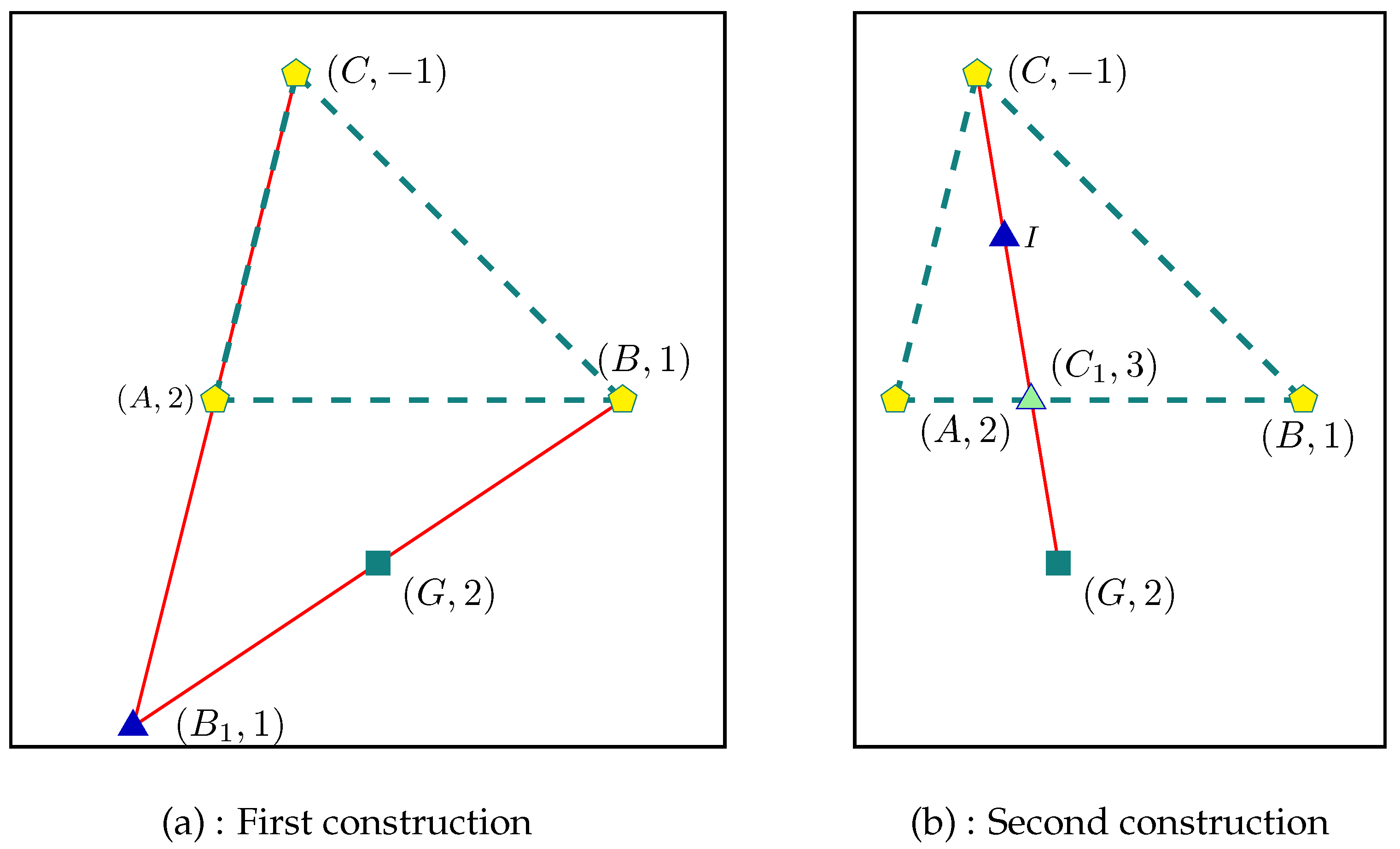
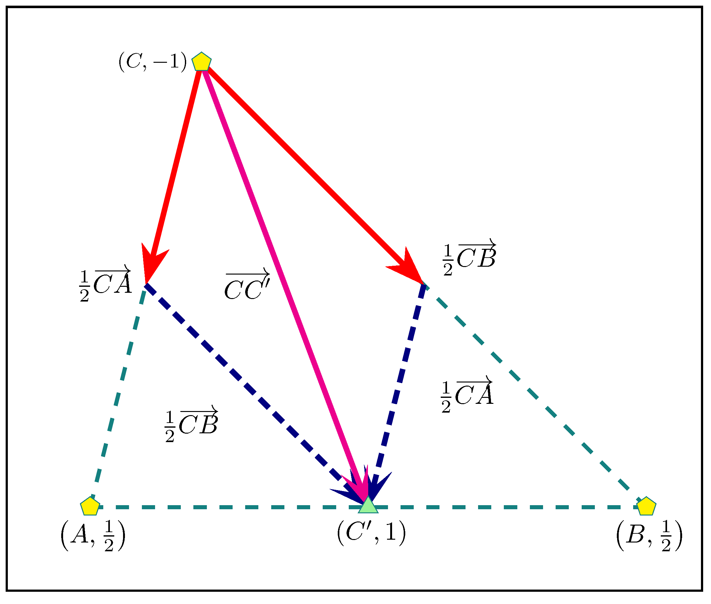
- Second construction. Let us introduce the barycenter of the weighted points and , i.e., is one-third of the way along the segment starting from A (see G in Figure 1). Then, is the barycenter of , , i.e., G is the symmetric of the midpoint I of the segment with respect to the point (see in Figure 2) (Figure 4b).
- 3.
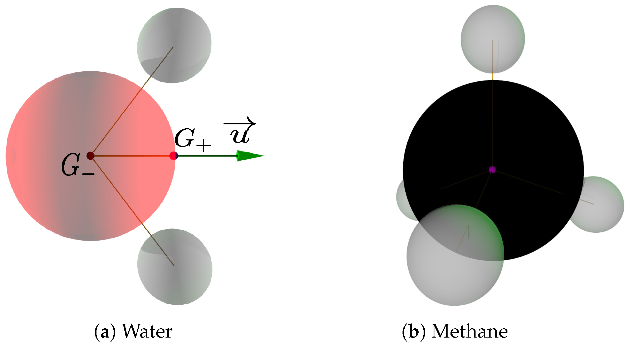
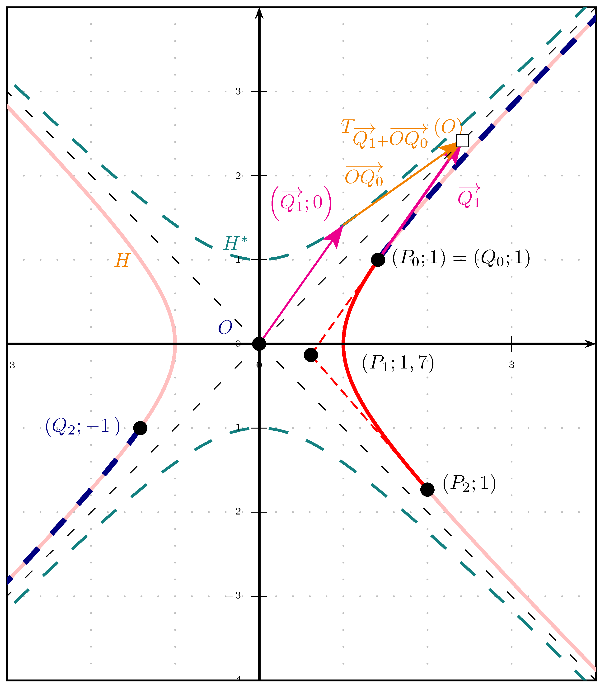
- Third construction. The weighted points and define the vector with a null mass. Then, there is the relationship between the points A and G and the vector : G is the image of A under the translation by the vector (Figure 5).
- ⋆
- If , then the denominator vanishes exactly once and the conic is a parabola;
- ⋆
- If , then the denominator does not vanish and the conic is an ellipse;
- ⋆
- If , then the denominator vanishes twice and the conic is a hyperbola.
- A cylinder of revolution has no singular point but contains the point at infinity;
- A cone of revolution has a singular point M, the apex, and the point at infinity;
- A spindle or horned Dupin cyclide has two singular points M and N;
- A one-singularity spindle or singly horned Dupin cyclide has only one singular point M.
- A circular cylinder if .
- A circular cone if . If , the apex is between the spheres and , i.e., there is such that a mass point of the Bézier curve representing this cone is a vector.
- Trace the segment starting from A with a zero velocity and arriving at B with a zero velocity;
- Trace the segment starting from B with a zero velocity and arriving at C with a zero velocity;
- Trace the segment starting from C with a zero velocity and arriving at A with a zero velocity.
2. Rational Bézier Curves in
- ;
- , where the notation denotes the barycenter of the weighted points and ;
- ;
- , where is the translation of of vector .
- ;
- ;
- .
- If , then
- If , then
2.1. Modeling Euclidean Circular Arcs with Mass Points
- If is not the midpoint of the segment ,let be the midpoint of the segment .The point is defined aswhere • is the usual dot product.The is a circular arc iff
- If is the midpoint of the segment , the is a semicircle of iff
2.2. Circles, Pseudo-Circles, Central Conics and Mass Points
3. The Null Vector in a Bézier Representation with Mass Points
- Second, the section ends with a natural behavior of null vectors obtained in the expression of a power curve in a BR form.
3.1. Differential Properties of Bézier Curves at 0 and 1 and Stationary Points
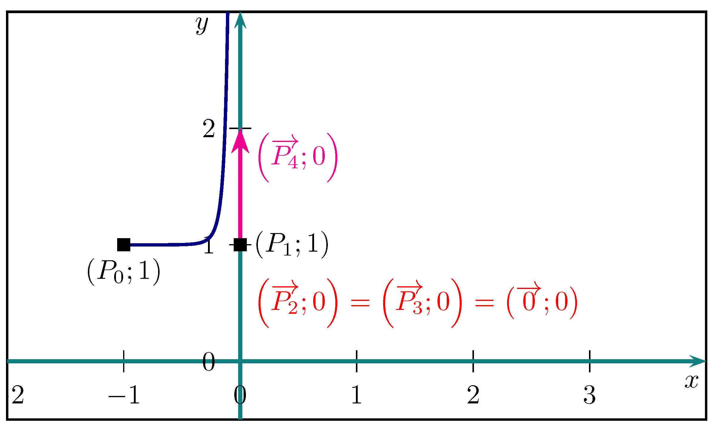
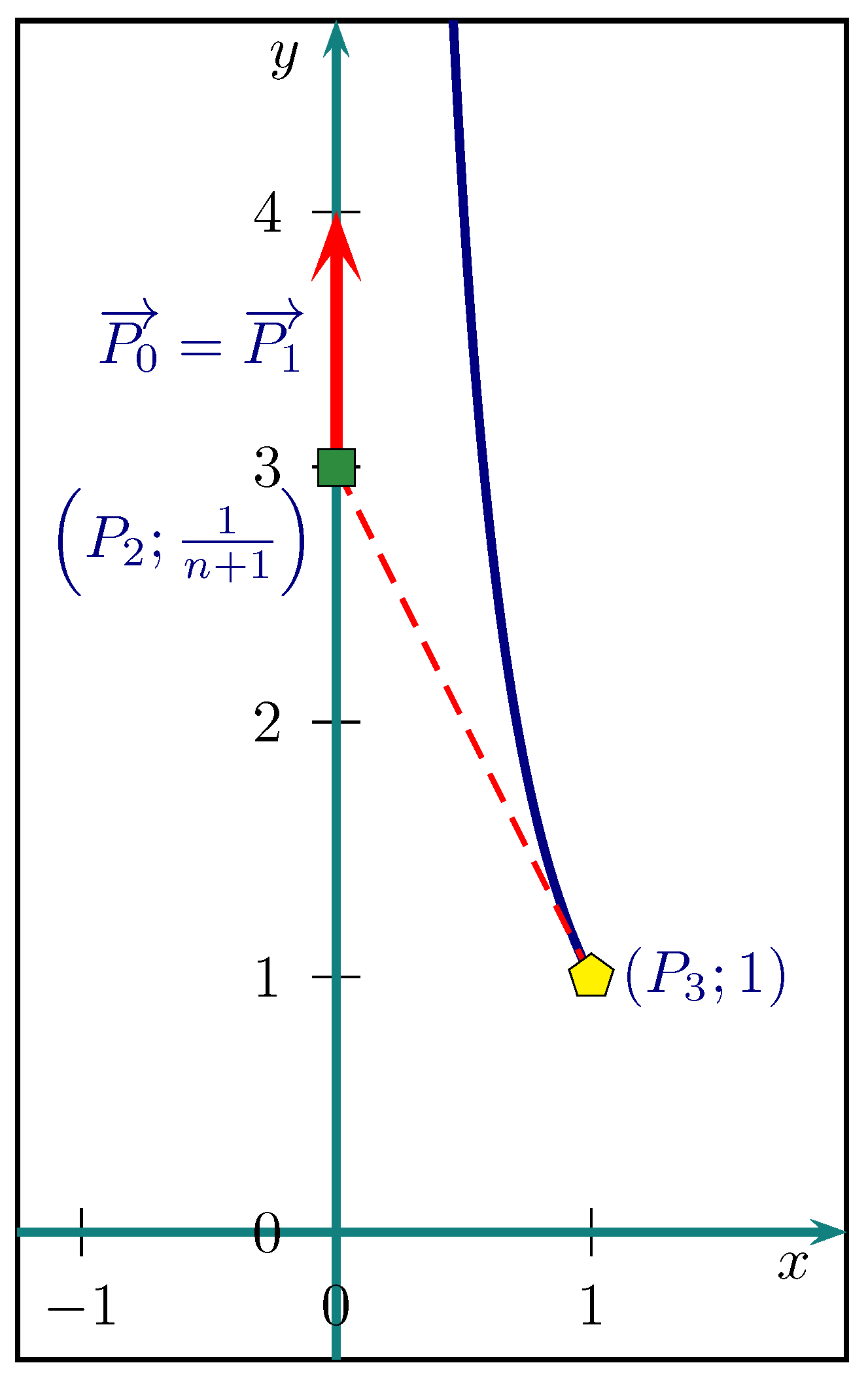
- If , the velocity vector of the curve at is given by
- If , the velocity vector of the curve at is given by
- If , the velocity vector of the curve at is given by
- If , the velocity vector of the curve at is given by
3.2. The Null Vector and Stationary Points at the Endpoints of a Segment
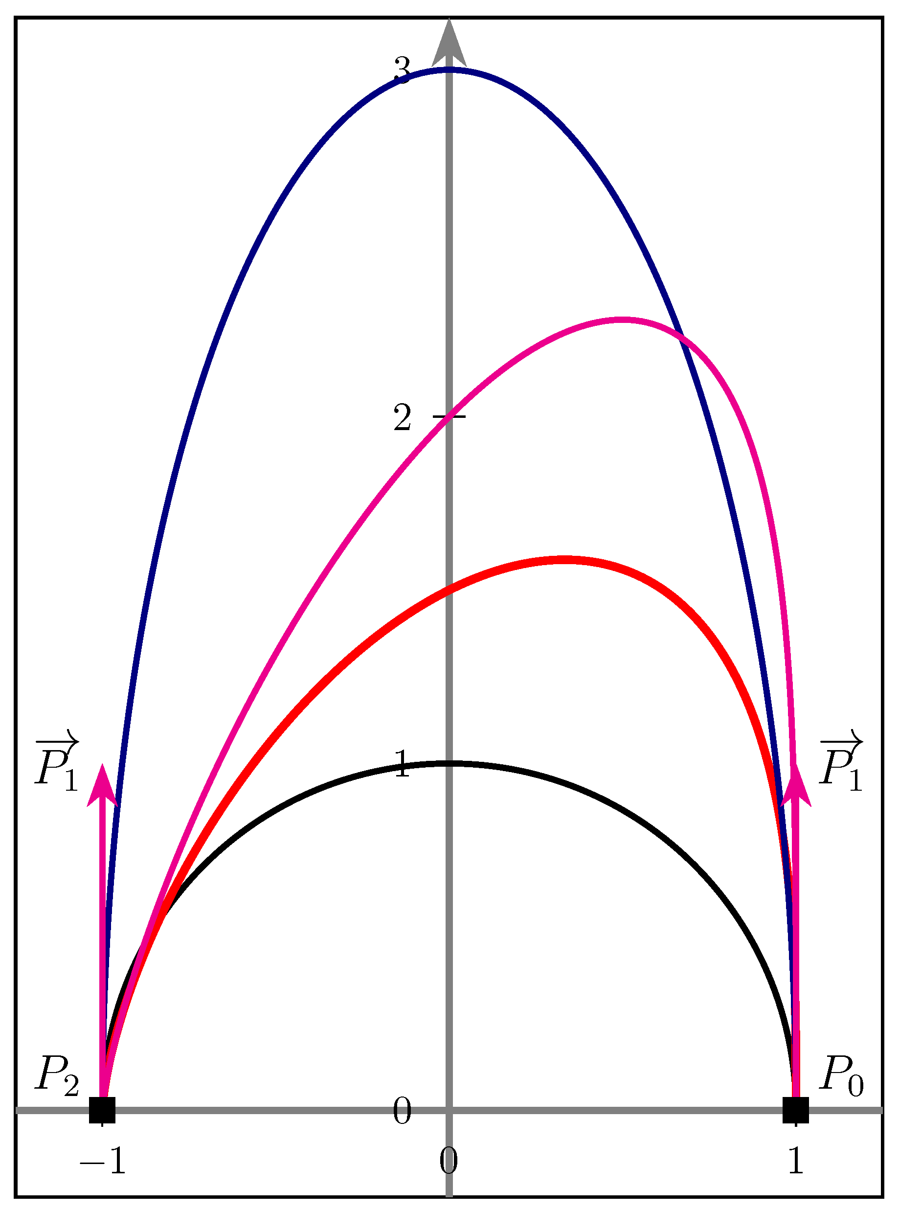
- 1.
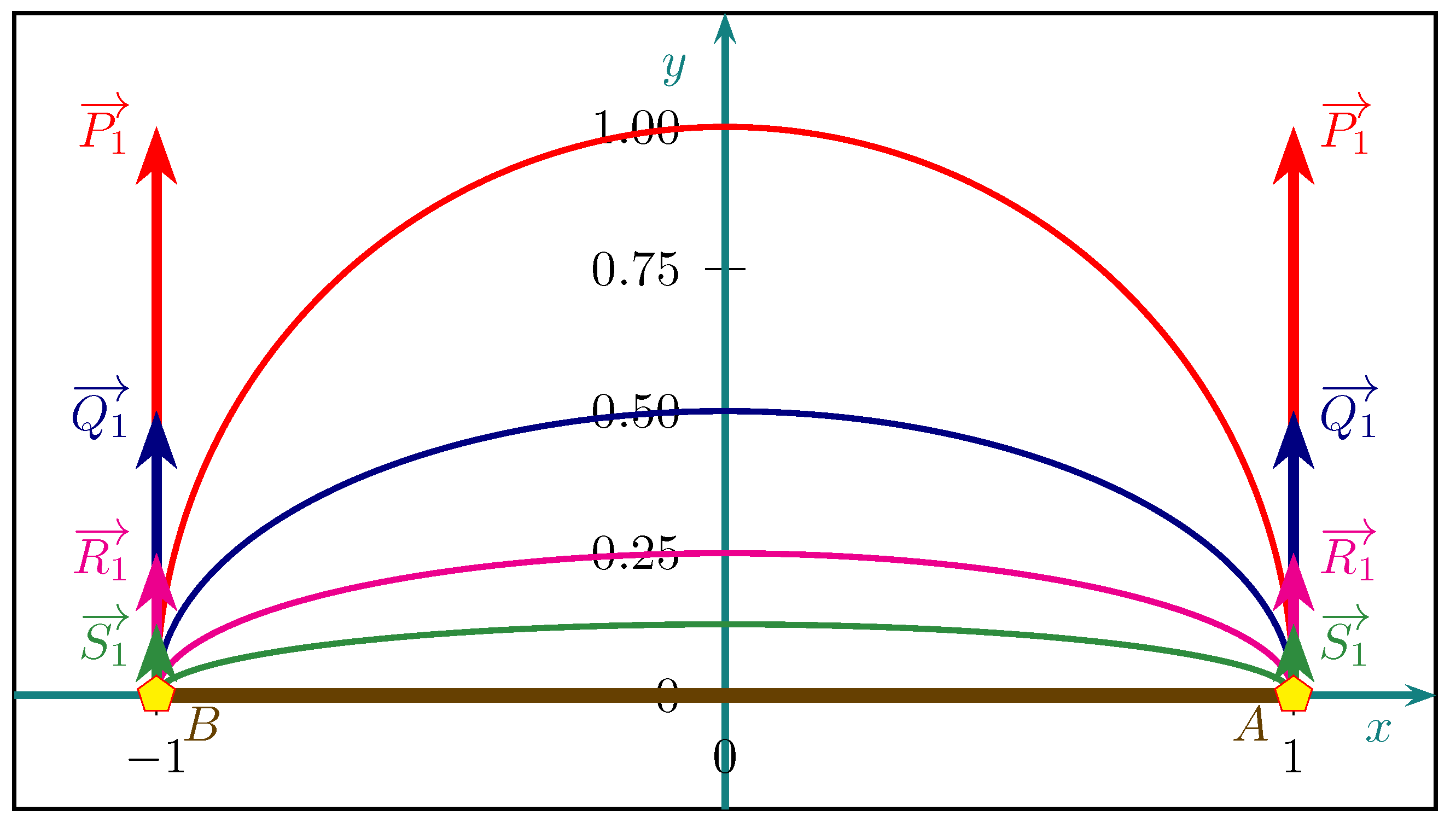
- with for the semicircle in red.
- 2.
- for the semi-ellipse in blue.
- 3.
- for the semi-ellipse in magenta.
- 4.
- for the semi-ellipse in green.
- 5.
- for the segment . The bounds are stationary points.
3.3. Quadratic Parameter Change for Kinematic
3.4. Multiple Vectors Performed in the Power Curve or the Inverse Power Curve
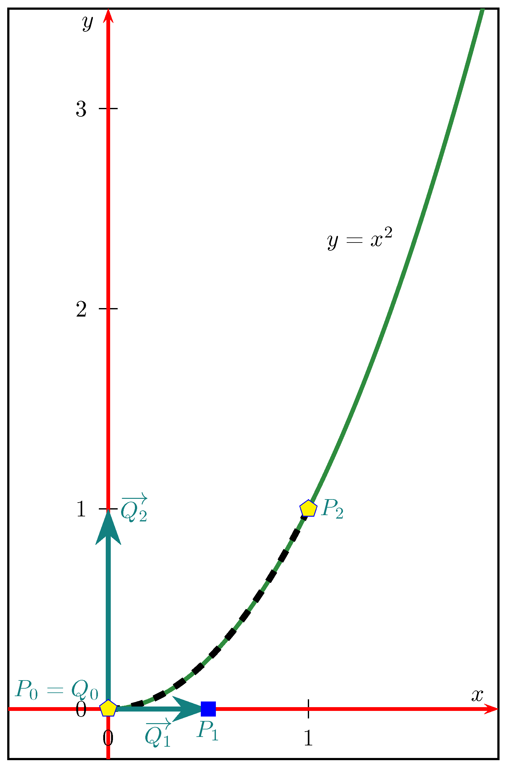
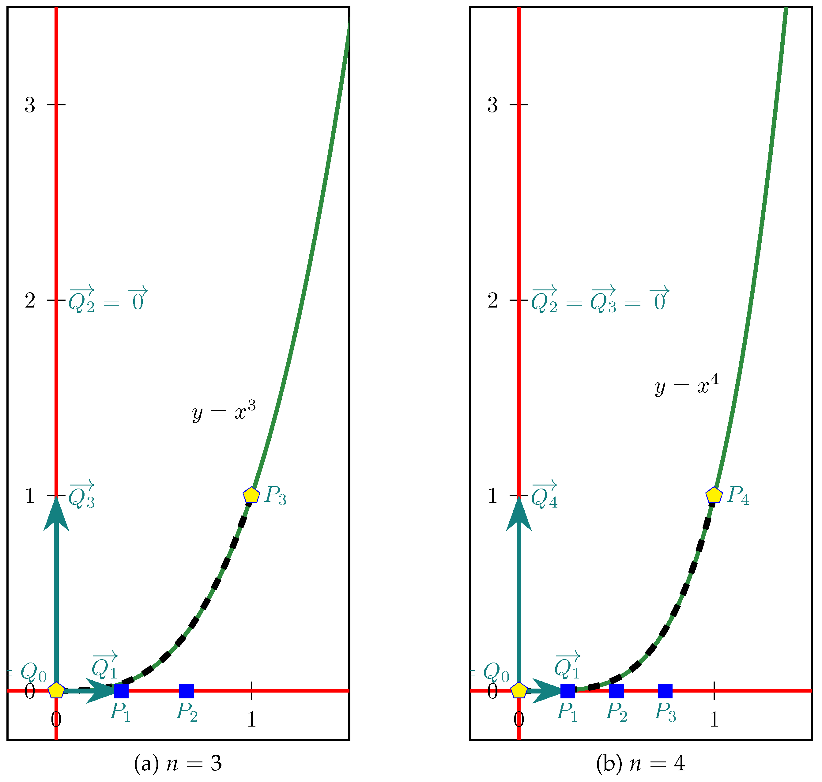
3.4.1. Multiple Null Vectors Performed in the Power Curve
3.4.2. An Example of a Bounded Area
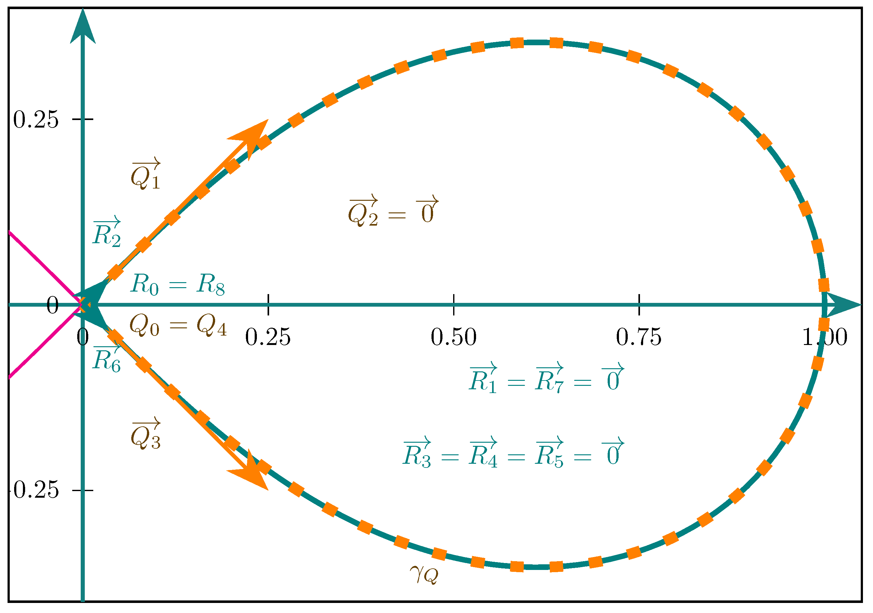
- weights and ;
- vectors , , ;
- and points and .
3.4.3. Multiple Vectors in the Inverse Power Curve
3.5. Stationary Points and Null Vectors
3.6. Segment and Kinematics
4. Examples of Two Stationary Endpoints
4.1. Case of Quadratic Curves
4.1.1. Quarter Circle Case
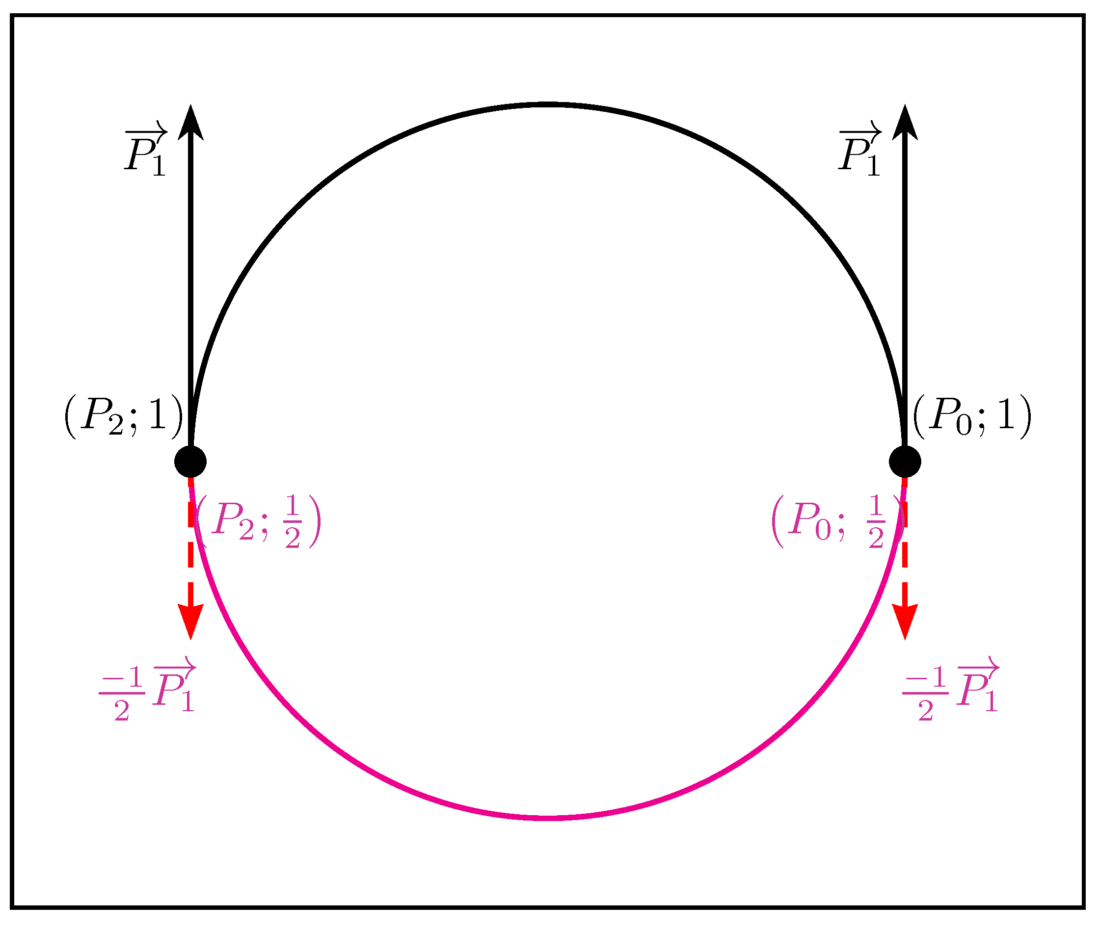
4.1.2. Half a Circle Case
4.2. Case of a Quartic Curve
4.3. Case of Canonical Bernouilli Lemniscate
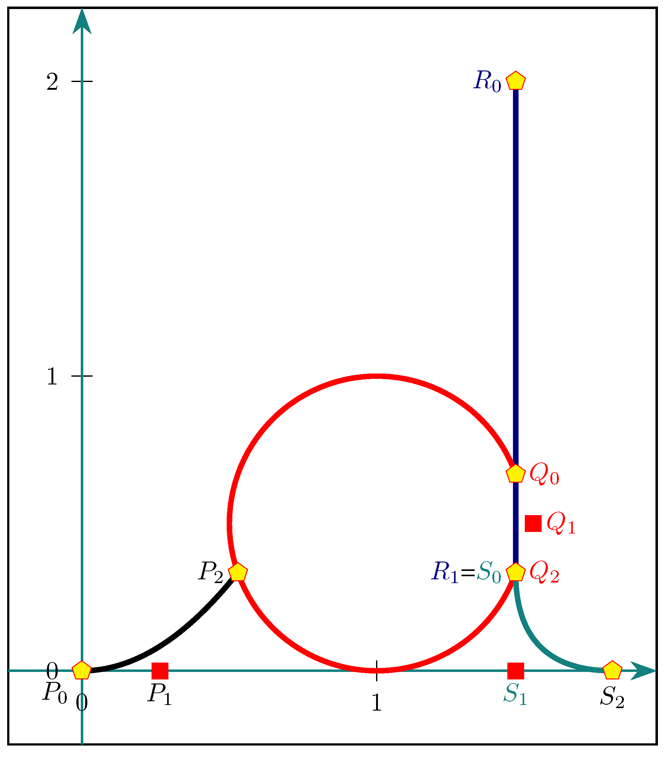
Construction of the Letter d
- 1.
- is an arc of a parabola, and the control mass points of the quadratic Bézier curve are , and ;
- 2.
- is an arc of a circle, and the three control mass points of the quadratic Bézier curve are , and ;
- 3.
- is the segment, and the control mass points of the Bézier curve of degree are and ;
- 4.
- is an arc of a parabola, and the control mass points of the quadratic Bézier curve are , and .
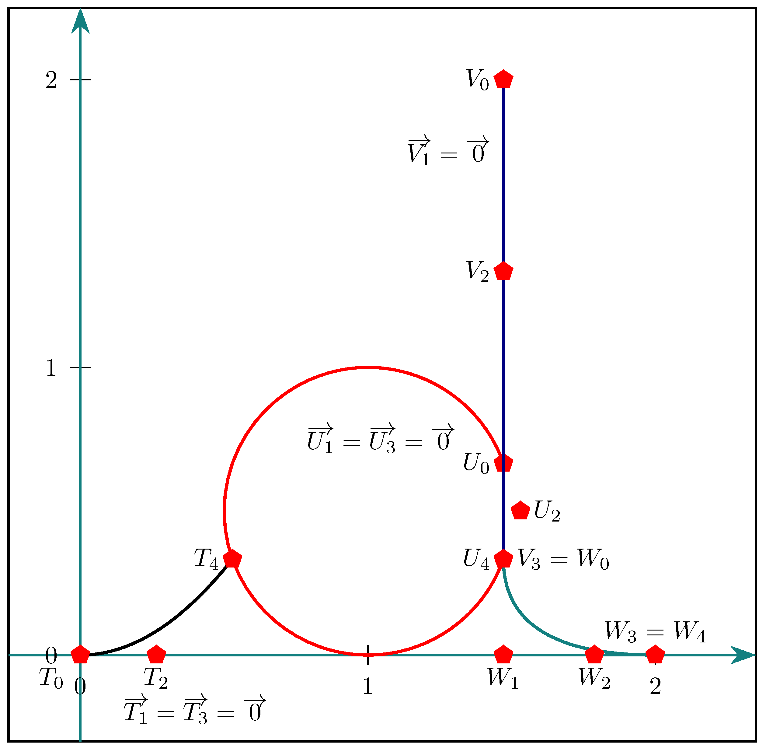
- 1.
- is an arc of a parabola and the control mass points of the quartic Bézier curve are , , , and ;
- 2.
- is an arc of a circle and the five control mass points of the quartic Bézier curve are , , , and ;
- 3.
- The control mass points of the cubic Bézier curve are , , and ;
- 4.
- is a parabola arc and the control mass points of the quartic Bézier curve are , , , and .
5. Conclusions and Perspectives
Author Contributions
Funding
Data Availability Statement
Conflicts of Interest
Appendix A. Examples of Computations with Mass Points
Appendix B. Formulae for the Degree 2
Appendix C. Formulae for the Degree 3
Appendix D. Formulae for the Degree 4
References
- Bézier, P. Courbe et Surface, 2nd ed.; Hermès: Paris, France, 1986; Volume 4. [Google Scholar]
- Farin, G. Curves and Surfaces for CAGD: A Practical Guide; Computer Graphics and Geometric Modeling, Elsevier Science: Amsterdam, The Netherlands, 2002. [Google Scholar]
- Farin, G. From Conics to NURBS: A Tutorial and Survey. IEEE Comput. Graph. Appl. 1992, 12, 78–86. [Google Scholar] [CrossRef]
- Ramshaw, L. Blossoms are polar forms. Comput. Aided Geom. Des. 1989, 6, 323–358. [Google Scholar] [CrossRef]
- Casteljau, P.D. Mathématiques et CAO. Volume 2: Formes à pôles; Hermes: Paris, France, 1985. [Google Scholar]
- Farin, G. NURBS from Projective Geometry to Pratical Use, 2nd ed.; A K Peters, Ltd.: Natick, MA, USA, 1999; ISBN 1-56881-084-9. [Google Scholar]
- Müller, A. Paul de Casteljau: The story of my adventure: From an autobiographical letter. Comput. Aided Geom. Des. 2024, 110, 102278. [Google Scholar] [CrossRef]
- Fiorot, J.C.; Jeannin, P. Courbes et Surfaces Rationnelles; Dunod: Paris, France, 1989; Volume RMA 12, Masson. [Google Scholar]
- Fiorot, J.C.; Jeannin, P. Courbes Splines Rationnelles, Applications à la CAO; Dunod: Paris, France, 1992; Volume RMA 24, Masson. [Google Scholar]
- Goldman, R. On the algebraic and geometric foundations of computer graphics. ACM Trans. Graph. 2002, 21, 52–86. [Google Scholar] [CrossRef]
- Ju, T.; Goldman, R. Morphing Rational B-spline Curves and Surfaces Using Mass Distributions. In Proceedings of the Eurographics, San Diego, CA, USA, 26–27 July 2003. [Google Scholar]
- Goldman, R. Understanding quaternions. Graph. Model. 2011, 73, 21–49. [Google Scholar] [CrossRef]
- Garnier, L. Courbes de Bézier quadratiques et coniques. Feuille Vigne Irem Dijon 2009, 113, 17–32. [Google Scholar]
- Piegl, L.; Tilles, W. A Managerie of Rational B-Spline Circles. IEEE Comput. Graph. Appl. 1989, 9, 46–56. [Google Scholar] [CrossRef]
- Gourion, M. Mathématiques, Terminales C et E, tome 2; Fernand Nathan: Manchester, UK, 1983. [Google Scholar]
- Ladegaillerie, Y. Géométrie Pour le CAPES de Mathématiques; Ellipses: Paris, France, 2002; ISBN 2-7298-1148-6. [Google Scholar]
- Ladegaillerie, Y. Géométrie Affine, Projective, Euclidienne et Anallagmatique; Ellipses: Paris, France, 2003; ISBN 2-7298-1416-7. [Google Scholar]
- Piegl, L. On the use of infinite control points in CAGD. Comput. Aided Geom. Des. 1987, 4, 155–166. [Google Scholar] [CrossRef]
- Bécar, J.; Fuchs, L.; Garnier, L. Courbe d’une fraction rationnelle et courbes de Bézier à points massiques. In Proceedings of the GTMG 2019, Toulouse, France, 28–31 October 2019. [Google Scholar]
- Bécar, J.P.; Garnier, L. Points massiques, courbes de Bézier quadratiques et coniques: Un état de l’art. In Proceedings of the G.T.M.G. 2014, Lyon, France, 26–27 August 2014. [Google Scholar]
- Garnier, L.; Bécar, J.P. Mass points, Bézier curves and conics: A survey. In Proceedings of the Eleventh International Workshop on Automated Deduction in Geometry, Strasbourg, France, 26–28 June 2016; Proceedings of ADG 2016. pp. 97–116. Available online: http://ufrsciencestech.u-bourgogne.fr/$\sim$garnier/publications/adg2016/ (accessed on 2 October 2024).
- Garnier, L.; Bécar, J.P.; Druoton, L. A Survey of De Casteljau Algorithms and Regular Iterative Constructions of Bézier Curves with Control Mass Points. WSEAS Trans. Math. 2024, 23, 216–236. [Google Scholar] [CrossRef]
- Bécar, J.P. Forme (BR) des Coniques et de Leurs Faisceaux. Ph.D. Thesis, Université de Valenciennes et de Hainaut-Cambrésis, Valenciennes, France, 1997. [Google Scholar]
- Piegl, L.A.; Tiller, W. The NURBS Book; Monographs in visual communication; Springer: Berlin/Heidelberg, Germany, 1995. [Google Scholar]
- Garnier, L.; Bécar, J.P.; Druoton, L. Canal surfaces as Bézier curves using mass points. Comput. Aided Geom. Des. 2017, 54, 15–34. [Google Scholar] [CrossRef]
- Garnier, L. Modélisation, Dans l’espace des Sphères, de Surfaces Canal par des Courbes de Bézier à l’aide de Points Massiques; Habilitation à diriger des recherches, Université de Bourgogne: Dijon, France, 2023. [Google Scholar]
- Langevin, R.; Sifre, J.C.; Druoton, L.; Garnier, L.; Paluszny, M. Finding a cyclide given three contact conditions. Comput. Appl. Math. 2014, 34, 275–292. [Google Scholar] [CrossRef]
- Druoton, L.; Langevin, R.; Garnier, L. Blending canal surfaces along given circles using Dupin cyclides. Int. J. Comput. Math. 2013, 91, 641–660. [Google Scholar] [CrossRef]
- Garnier, L.; Bécar, J.P. Nouveaux Modèles Géométriques pour la C.A.O. et la Synthèse D’images: Courbes de Bézier, Points Massiques et Surfaces Canal; Editions Universitaires Européennes: Saarbrucken, Germany, 2017; ISBN 978-3-639-54676-7. [Google Scholar]
- Garnier, L.; Bécar, J.; Druoton, L.; Fuchs, L.; Morin, G. Theory of Minkowski-Lorentz Spaces. In Encyclopedia of Computer Graphics and Games; Lee, N., Ed.; Springer: Berlin/Heidelberg, Germany, 2019. [Google Scholar] [CrossRef]
- Garnier, L.; Bécar, J.; Druoton, L.; Fuchs, L.; Morin, G. Minkowski-Lorentz Spaces Applications: Resolution of Apollonius and Dupin Problems. In Encyclopedia of Computer Graphics and Games; Lee, N., Ed.; Springer International Publishing: Cham, Switzerland, 2020; pp. 1–10. [Google Scholar] [CrossRef]
- Garnier, L.; Bécar, J.P.; Morin, G.; Fuchs, L. Une Application de L’espace des Sphères: Détermination des sphères de Dandelin; Université de Lyon: Lyon, France, 2015. [Google Scholar]
- Garnier, L.; Druoton, L.; Bécar, J.; Fuchs, L.; Morin, G. Subdivisions of Ring Dupin Cyclides Using Bézier Curves with Mass Points. WSEAS Trans. Math. 2021, 20, 581–596. [Google Scholar] [CrossRef]
- Garnier, L.; Druoton, L.; Bécar, J.; Fuchs, L.; Morin, G. Subdivisions of Horned or Spindle Dupin Cyclides Using Bézier Curves with Mass Points. WSEAS Trans. Math. 2021, 20, 756–776. [Google Scholar] [CrossRef]
- Garnier, L.; Druoton, L.; Bécar, J.; Fuchs, L.; Morin, G. Mass Points, Spaces of Spheres, “hyperbolae” and Dandelin and Quételet Theorems. WSEAS Trans. Math. 2022, 21, 285–302. [Google Scholar] [CrossRef]
- Garnier, L. Mathématiques pour la Modélisation Géométrique, la Représentation 3D et la Synthèse D’images; Ellipses: Paris, France, 2007; ISBN 978-2-7298-3412-8. [Google Scholar]
- Garnier, L.; Bécar, J.; Druoton, L.; Fuchs, L.; Morin, G. Pencils of Spheres in the Minkowski-Lorentz Spaces. In Encyclopedia of Computer Graphics and Games; Lee, N., Ed.; Springer: Berlin/Heidelberg, Germany, 2024. [Google Scholar]
- Garnier, L. Résultat sur les Courbes de Bézier à Points Massiques de Contrôle. Working Paper or Preprint. Available online: https://u-bourgogne.hal.science/hal-04051237/ (accessed on 2 October 2024).


| Point 1 | Point 2 | Point 3 | Condition | Type |
|---|---|---|---|---|
| Semi-ellipse | ||||
| Parabola arc | ||||
| Parabola arc | ||||
| Semi-hyperbola | ||||
| Hyperbola branch |
| Point 1 | Point 2 | Point 3 | Kind of the Dupin Cyclide |
|---|---|---|---|
| Circular cylinder | |||
| Semicircular cone with apex M | |||
| Patch of Dupin cyclide with endpoints M and N |
| Conditions | Expression of , Formula (24) |
|---|---|
Disclaimer/Publisher’s Note: The statements, opinions and data contained in all publications are solely those of the individual author(s) and contributor(s) and not of MDPI and/or the editor(s). MDPI and/or the editor(s) disclaim responsibility for any injury to people or property resulting from any ideas, methods, instructions or products referred to in the content. |
© 2025 by the authors. Licensee MDPI, Basel, Switzerland. This article is an open access article distributed under the terms and conditions of the Creative Commons Attribution (CC BY) license (https://creativecommons.org/licenses/by/4.0/).
Share and Cite
Garnier, L.; Bécar, J.-P.; Fuchs, L. How Null Vector Performs in a Rational Bézier Curve with Mass Points. Geometry 2025, 2, 1. https://doi.org/10.3390/geometry2010001
Garnier L, Bécar J-P, Fuchs L. How Null Vector Performs in a Rational Bézier Curve with Mass Points. Geometry. 2025; 2(1):1. https://doi.org/10.3390/geometry2010001
Chicago/Turabian StyleGarnier, Lionel, Jean-Paul Bécar, and Laurent Fuchs. 2025. "How Null Vector Performs in a Rational Bézier Curve with Mass Points" Geometry 2, no. 1: 1. https://doi.org/10.3390/geometry2010001
APA StyleGarnier, L., Bécar, J.-P., & Fuchs, L. (2025). How Null Vector Performs in a Rational Bézier Curve with Mass Points. Geometry, 2(1), 1. https://doi.org/10.3390/geometry2010001