Longitudinal Investigation of Groundwater and Surface Water Interaction of Two Gravel Pit Lakes in Central Texas: Chemical and Flow Implications

Abstract

Two gravel pit lakes in central Texas were examined over the course of two years with upgradient and downgradient piezometer installations. Groundwater and lake water were sampled bimonthly for nutrients, water levels, and groundwater chemistry, and in addition, rain and lake gauges and mini-piezometers were installed, depth surveys were conducted, and a simple 2D flow model was constructed. The project goal was evaluating and examining flow dynamics and chemical effects as groundwater flows to surface water and back to groundwater with the intent to understand the effects that gravel pit lake systems have on connected shallow groundwater. Both lake systems were shown to be flow-through systems that influence the water quality by decreasing the dissolved nutrients in the groundwater in their vicinity while oxygenating the water and altering the pH. However, the lakes are also prone to high levels of evaporation, meaning that minor improvements to water quality come at the cost of decreasing the quantity of water in storage within the aquifer. Similar groundwater and mine lake systems may show comparable tendencies, providing new information for water managers, regulators, and stake-holders about the potential roles that non-remediated gravel pit lakes may play in local ecosystems and aquifer dynamics.

1. Introduction

As the Texas population grows over the next few decades, demand for natural aggregate construction materials (crushed stone, gravel, sand, etc.) and water will increase simultaneously. The Texas population is projected to nearly double by 2050 (from 29 million to 50 million people) which will necessitate the large-scale construction of infrastructure and exacerbate problems already being experienced in the provision of water [1,2]. In central Texas, much of the sand and gravel used in construction material is mined using open pits in shallow alluvial aquifers. This study focuses on two former pit mines in one such aquifer, the Brazos River Alluvium Aquifer (BRAA), specifically the section within McLennan County near the City of Waco.

In the BRAA and other alluvial aquifers in Texas, aggregates in pit mines are frequently quite shallow corresponding to the thickness of the aquifer. The BRAA’s maximum thickness never exceeds 175 feet at its absolute thickest, and is much thinner in McLennan County, averaging around 35 feet thick [3]. The BRAA is generally characterized as being composed of alluvial sediments that exhibit a fining upward sequence. The alluvial sediments that form the aquifer range in size from extremely coarse limestone and chert gravel to medium sands to clays. The large gravels and coarse sands are typically the goal in mining operations. When observed at the local scale, the geometry of sediments can be extremely complex after years of reworking by the river. In the study area, there are terraced deposits of various particle sizes with sediments showing partial fining upward sequences in succession and non-laterally extensive but with frequent lenses of clay and silt. Despite this complexity, in many cases most of the materials that would be viable for mining are in the lower layers of the aquifer, below the water table [3,4]. This leads to pit mines that intersect the water table where the coarse aquifer material is removed. In Texas, it is common for these types of pits to be left unremediated and allowed to fill with water from the aquifer, equilibrating to the water table surface elevation, and forming a “gravel pit lake” (GPL). These lakes are frequently used as water features for recreation or to provide a reliable water source for livestock. Owners often stock the lakes with fish which provide incentive for birds and other animals to nest nearby. Given enough time, a GPL eventually can grow to resemble a naturally occurring groundwater-fed lake, complete with a lacustrine ecosystem [5].

The effects of GPLs on groundwater systems vary widely; sometimes they can serve as point sources of aquifer contamination through surface runoff and atmospheric deposition while at other times they might provide a site for the bioremediation for nutrients [6,7]. GPLs also have varying effects on the evaporation regimes within the aquifer which can alter the flow dynamics of the system locally [8]. Previous studies have shown that the banks, flora, and fauna, as well as the size of the lake and the mineralogy of the aquifer system, all play a role in their effects on the groundwater [7,9,10,11,12]. However, few studies have examined small-scale lakes in thinner aquifers in dry regions. The primary goal of this study is to characterize the local aquifer and groundwater effects of small GPLs on the BRAA to help guide the future management, regulation, and monitoring of such lakes as their numbers continue to multiply with increasing demand for mined aggregate materials. This study also seeks to begin to fill the literature gap surrounding GPLs in shallow unconfined aquifers, particularly in Texas, where their effects remain largely unexplored.

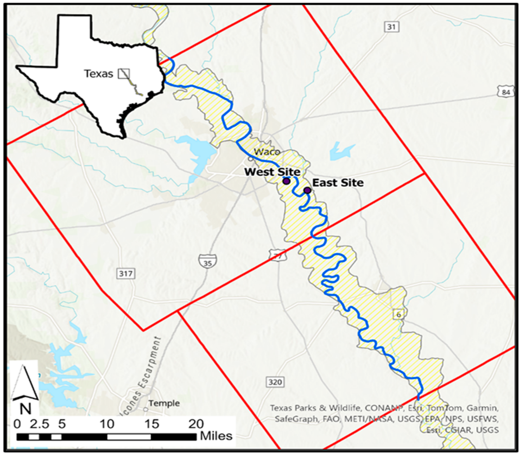
This study focuses on two GPLs in the northern segment of the BRAA in McLennan County Texas (Figure 1).

The BRAA is a Quaternary emplacement of riverine sediments, a mix of clay, silt, sand, and gravel. The BRAA is typically characterized as a large fining upward sequence; however, the aquifer sediments are terraced in some locations leading to repetition of some sediment types where the aquifer is thicker. Beyond this, the local stratigraphic architecture in a given area may be quite complex, with lenses of gravel and sand creating perched water tables and clays that can be saturated and yet produce little to no water [13]. In the Pleistocene, the Brazos River was much larger, with discharges equaling between five to eight times current amounts. This larger volume of water during interglacial periods led to broad floodplains which were continually dissected and reworked as glacial fluctuations occurred, leading to a complex mélange of stratified alluvial sediments across the entire aquifer [14]. This complexity complicates modeling the aquifer. Some parts of the aquifer are more permeable and exhibit quicker flow paths than do others [15]; this has the potential to cause GPLs to function differently depending on their location within the aquifer, making the lake location within the BRAA an important consideration for future work in monitoring and for developing a regulatory framework.

The northern segment of the BRAA is characterized by thinner aquifer sediments and a shallower water table than that which occurs in the lower sections of the aquifer. The northern segment also features compartmentalization to a higher degree than the lower sections of the aquifer. In the BRAA, compartmentalization is due to the Brazos River intersecting low-permeability bedrock in some stream reaches. When the river channel intersects the bedrock, lateral aquifer flow is essentially cut off from one side of the aquifer to the other as the river channel serves as a hydrologic divide [16]. The bedrock is cretaceous aged chalk and marls and is not known to contribute appreciable volumes of water to the BRAA [13]. This compartmentalization is important to document because the two selected lakes in this study are on opposite sides of the Brazos in a stream reach that is bedrock dominated and can be considered to be impacted by independent flow systems [16]. This could have implications for the development of our understanding of gravel pit lakes. For the duration of this study, conditions in both lakes were similar. Such similar conditions are not guaranteed, particularly considering future climatic shifts towards dryness in the region [17] and differences in local deposition between the two compartments.

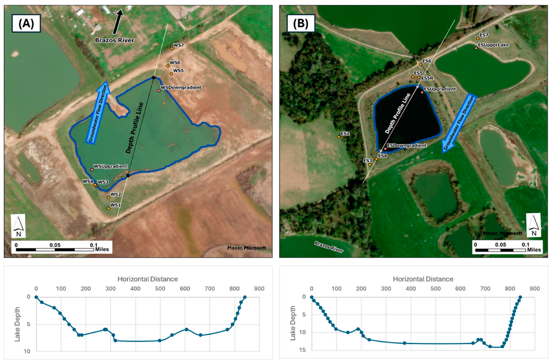
The two lakes are similar in terms of the observations made during this study but occur in two separate compartments of the BRAA which are divided from one another by the Brazos River acting as a hydrologic boundary [16]. At the time studied, both lakes were similar in terms of lateral dimensions with Lake 1 ranging from 420,000–450,000 sq feet (or 10 acres) (depending on water level), while Lake 2 had dimensions ranging from 380,000 to 390,000 sq feet (or nine acres). Both lakes showed similarly shaped depth profiles in the aquifer flow direction (Figure 2).

The West Site lake had a maximum depth of about eight feet while the East Site lake had a maximum depth of about 14 feet. These depths are snapshots determined by lake depth measurements on a single trip to each site; the depths of the lakes, like their horizontal dimensions, are somewhat dependent on precipitation patterns, water table level, and drought conditions.

2. Materials and Methods

This study used a variety of hydrogeology field and lab techniques to characterize and explore the local aquifer effects that the GPLs have in the BRAA. Subsections describe chemical sampling methodologies, field methodologies, and modeling methodology, respectively.

2.1. Sampling Methods

Prior to long-term monitoring, two-inch diameter piezometers were installed on both the up- and downgradient sides of each lake (Figure 3D–F) using completion methods described in hydrogeology field guides [18,19].

Piezometers were arranged in a line in the interpolated flow direction of the BRAA aquifer (using groundwater contours and considering the Brazos River as the low point and interpreting a perpendicular line as the direction of groundwater flow) (Figure 2). Piezometers were installed using a Geoprobe 6620 DT drill rig with 3.25 inch diameter hollow stem auger flight (Geoprobe Systems Inc., Salina, KS, USA). Boreholes were augured to between 10 feet and 15 feet below the saturated zone in the aquifer, depending on the elevation difference between the top of the of saturated zone and the top of the bedrock on a per-hole basis. Piezometers were fully assembled before placement in boreholes. To reduce hole collapse during assembly, the auger flight was temporarily left in the boreholes until the well casing and screen were assembled. Piezometer length and screen length were dependent on the depth to the saturated zone. Piezometers were constructed from two-inch diameter interlocking PVC pipe with a pointed end cap. Each section of pipe measured 10 feet. The top section of each piezometer was sawed off after installation to minimize its surface visibility. Well screens were factory-machined PVC that used 0.02 inch slots. Screen lengths for all piezometers were dependent on the estimated elevation of the saturated zone but averaged 10 feet. After the piezometer was constructed and inserted into the borehole, the Geoprobe was used to push the screen into the saturated zone as completely as possible. Filter sand was used as a sand pack around the screen where necessary and when full insertion of the screen into the aquifer material was impossible. Bentonite pellets were poured into each borehole above the screen to serve as a plug after the filter sand. The remaining space in each borehole was then backfilled with construction sand. Piezometers were bailed between 30 to 50 times to help develop the material around the screen and reduce suspended sediment in future sampling. Auger cuttings were logged during drilling along with depths to provide insight about the nature of the aquifer material and saturated zone in each borehole. These cutting logs were used to construct piezometer diagrams (Figure 4) which were used for flow modeling in the aquifer.

Multiple types of water samples were taken from both the downgradient and upgradient sides of the lakes and from piezometers at different intervals over the course of the study. Standard ion samples and Oxygen-18 and Deuterium samples were collected in a 50 mL bottle at each piezometer and gravel pit lake. When collecting samples, there was no head space in the vials and the lids were taped closed. Isotope samples were analyzed using the Thermo-Electron Delta V Advantage Isotope Ratio Mass Spectrometer (IRMS) (Thermo Fisher Scientific Inc., Waltham, MA, USA) in the stable isotope lab at Baylor University while ion samples were analyzed by Biochem Inc., West, TX, USA. Dissolved nitrate, ammonia, and phosphate samples were analyzed in the Baylor Center for Reservoir and Aquatic Systems Research. Nutrient water samples were extracted from wells and lakes using a bailer. Wells were bailed a minimum of three times per sample to ensure fresh groundwater was in the well. Lake water was sampled by tossing the bailer 50 feet towards the center of the lake. Water was then pushed through 0.45 micron polypropylene syringe filters into 50 mL centrifuge tubes. Tubes were rinsed with filtered sample water 3 times before being filled with the samples and put on ice. Samples were transported back to the lab in an ice chest and frozen until being run on a Lachat Instruments Quikchem 8500 (Lachat Instruments, Milwaukee, WI, USA). For isotope samples, the water was unfiltered and the first bail from the wells was used to obtain unagitated water. Isotope samples were drawn from the bottom of the bailer in 50 mL centrifuge tubes that were sealed with no head and taped to prevent atmospheric exchange. Ion samples were collected in 250 mL bottles. Anion samples were acidified with 5 ml of nitric acid for transport. Titrations were performed immediately at each well site using the same waters captured for ion samples to reduce the degassing effects that caused changes in alkalinity [18,19].

2.2. Field Methods

Mini-piezometers (Figure 3A) were installed around the perimeters of both gravel pit lakes to examine the influx of groundwater from the banks. Mini-piezometers were installed according to the methodologies outlined in hydrogeology field manuals and field exercise publications [18,19,20,21]. Five-foot sections of one-inch internal diameter PVC were slotted using a pipe saw. The PVC sections were inserted into galvanized pipes and a stainless-steel bolt was secured in the PVC to prevent the warping of the piezometers and the galvanized pipe from hammering. The galvanized pipes were hammered into bank sediments using a rubber mallet until at least two feet of the PVC was fully enclosed by bank sediments. The galvanized pipes were removed, leaving the PVC behind. After construction, the mini-piezometers were bailed until empty and allowed to equilibrate with bank sediment pore water conditions. The mini-piezometers were measured biweekly through the beginning stages of the study using a small gauge Solinst electrical line in order to examine the presence or absence of groundwater flow into the lakes via their banks.

Slug tests were performed [22] on one upgradient (WS2 and ES5R) and one downgradient (WS5 and ES4) full-size piezometer at each lake to evaluate local hydraulic conductivity values around each of the lakes and compare them to Freeze and Cherry to verify the validity of the parameters used in the TopoDrive and ParticleFlow 1.0 model. Slugs were fitted into piezometers and water levels were allowed to equilibrate over 24 h. Data loggers were fitted into the piezometers and set to record water levels every 10 s. After equilibration, slugs were removed, and water levels were measured by hand using a Solinst water level indicator (e-line) every 10 s until static conditions were observed.

Depth surveys were performed from a kayak using a lead-weighted steel tape. Three equidistant lines of marked and buoyant nautical ropes were placed across each lake. Depth measurements were taken at pre-marked 30-foot intervals along each line and boundary conditions were measured at 0-foot depths (immediately where the water touched the shore), and the depths of each lake were measured at 1 foot from the shore around the rim of each lake. Data were input into ArcGIS pro 3.1.3 and interpolated using the IDW method to produce depth estimates for each lake. Depth profiles were constructed using the interpolation surfaces in the direction of groundwater flow for each lake using a 1-foot interval (Figure 2).

Lake gauges were installed at both sites to measure the lake water level elevation in relation to that of the piezometers (Figure 3C). Lake gauges, piezometers, and other measurement points were surveyed using a Leica kinematic GPS to establish their elevation in relation to sea level. All elevations are reported referenced to sea level. An auto-recording tipping bucket rain gauge was installed near the West Lake site (Figure 3B) to record rainfall events and examine their correlation to water levels in both the aquifer and lake. A piezometer on the upgradient and downgradient sides of each lake was also fitted with a Solinst pressure transducer data logger that recorded the groundwater level in each piezometer on an hourly basis to enable closer inspection of groundwater levels as they responded to rainfall.

2.3. Modeling Methods

TopoDrive and ParticleFlow 1.0, a two-dimensional, steady-state, finite element model [23], were used to estimate the time it takes for groundwater to move through the aquifer and the gravel pit lakes at each site. The two-dimensional model domains were aligned with the interpolated groundwater flow direction and extended from the farthest upgradient piezometer to the Brazos River. At the West Site, the model domain length was set to 705 m with a vertical exaggeration of 30 times. At the East Site, the model domain length was set to 875 m with a vertical exaggeration of 30 times. The water table points were made based on groundwater measurements from piezometers and surface-water measurements were taken from the lake gauges at both sites; the river elevations used for this model were obtained from Google Earth Pro. It should be noted that the groundwater elevation between the river and the gravel pit lake was only measured from two piezometers that are near the gravel pit lake and is interpreted for the rest of the model based on the river elevation. The shape of the lake was input into the model based on lake depth surveys that were conducted at each site. At the West and East Sites, the mesh was made from 100 columns and 50 rows. The sediment layer depths were added to the model domains based on auger cuttings that were recorded when the piezometers were installed (Figure 4). Figure 5 shows the TopoDrive color and the corresponding sediment description, hydraulic conductivities, and porosities that were used at the West Site and East Site.

The hydraulic conductivity of each sediment layer is based on slug tests conducted on the upgradient and downgradient side of both gravel pit lakes using methods and calculations from Bouwer and Rice [22]; the hydraulic conductivity and porosity of the sediments were then referenced to hydraulic conductivity values for sediment types as calculated by Freeze and Cherry [24]. The vertical hydraulic conductivity values are based on the data from the Final Numerical Model Report for the Brazos River Alluvium Aquifer Groundwater Availability Model [25,26].

3. Results and Discussion

Water sampling took place from May 2021 to September 2022 at the West Site and from July 2021 to September 2022 at the East Site to capture a full warm and cool seasonal cycle. This area of central Texas typically has hot dry summers and cooler and wetter winters [27]. Mini-piezometers (MPs) in both lakes were monitored for two months during the dry season in order to investigate groundwater flow into the lakes from bank filtration. All MPs in both lakes showed a consistent loss of water to the bank from the lake (mini-piezometer water levels were lower than the lake level) [18,21]; however, the gradient steepened in the predicted direction of groundwater flow in both lakes. This indicates that although the lakes are losing water to banks, the gradient of the lakes follows that which was found in the full-size piezometers, supporting the notion that the lakes are flow-through systems, at least partially, and likely are more connected to the BRAA system at depth than in the near surface portion of their banks.

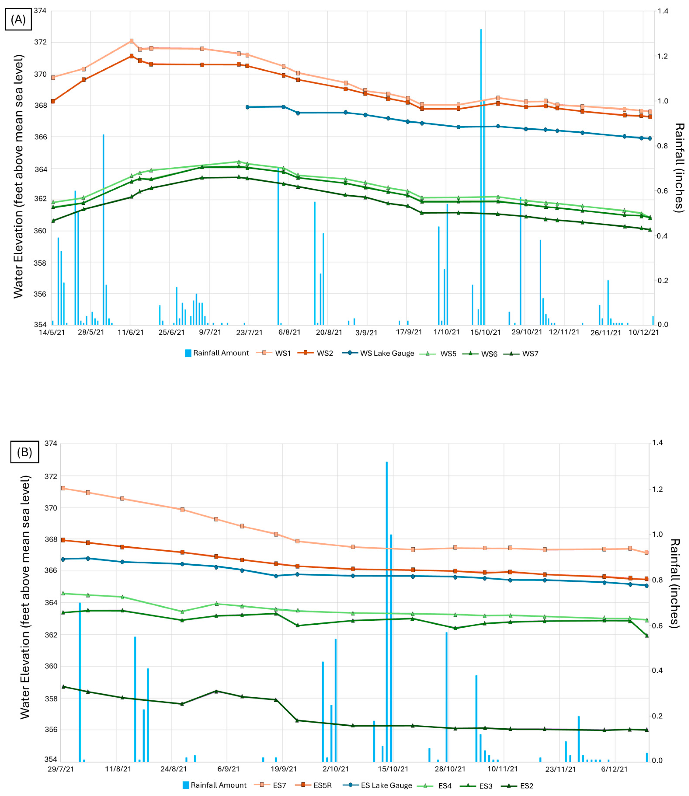
Hand-measured data from both lakes and all piezometers compared to the tipping bucket rain gauge are displayed in Figure 6 for the first 6 months of the study.

West Site lake levels and groundwater levels have a weak positive correlation with rainfall events. However, the East Site does not share this relationship. This may be due to the monitoring period available for the East Site, given that the summer and fall of 2021 were so dry in this area that the intermittent rainfall slowed the decline of groundwater levels, flattening the slopes of the hydrographs rather than prompting recharge events and raising groundwater levels. The slowdown in water level decline could also be partially influenced by a reduction in regional pumping in the BRAA during the rain events or some combination thereof. Lake levels appear to respond to rainfall no more or less dramatically than do the piezometers. The lakes’ water elevation consistently plots precisely where one might expect a piezometer’s water elevation to fall along the gradient rather than being influenced by rainfall events. The responses of lake levels and piezometer levels to rainfall events implies a relationship between groundwater and lake levels; however, with the data gathered as part of this project, there could be further confounding factors that make it difficult to identify trends at the biweekly scale. 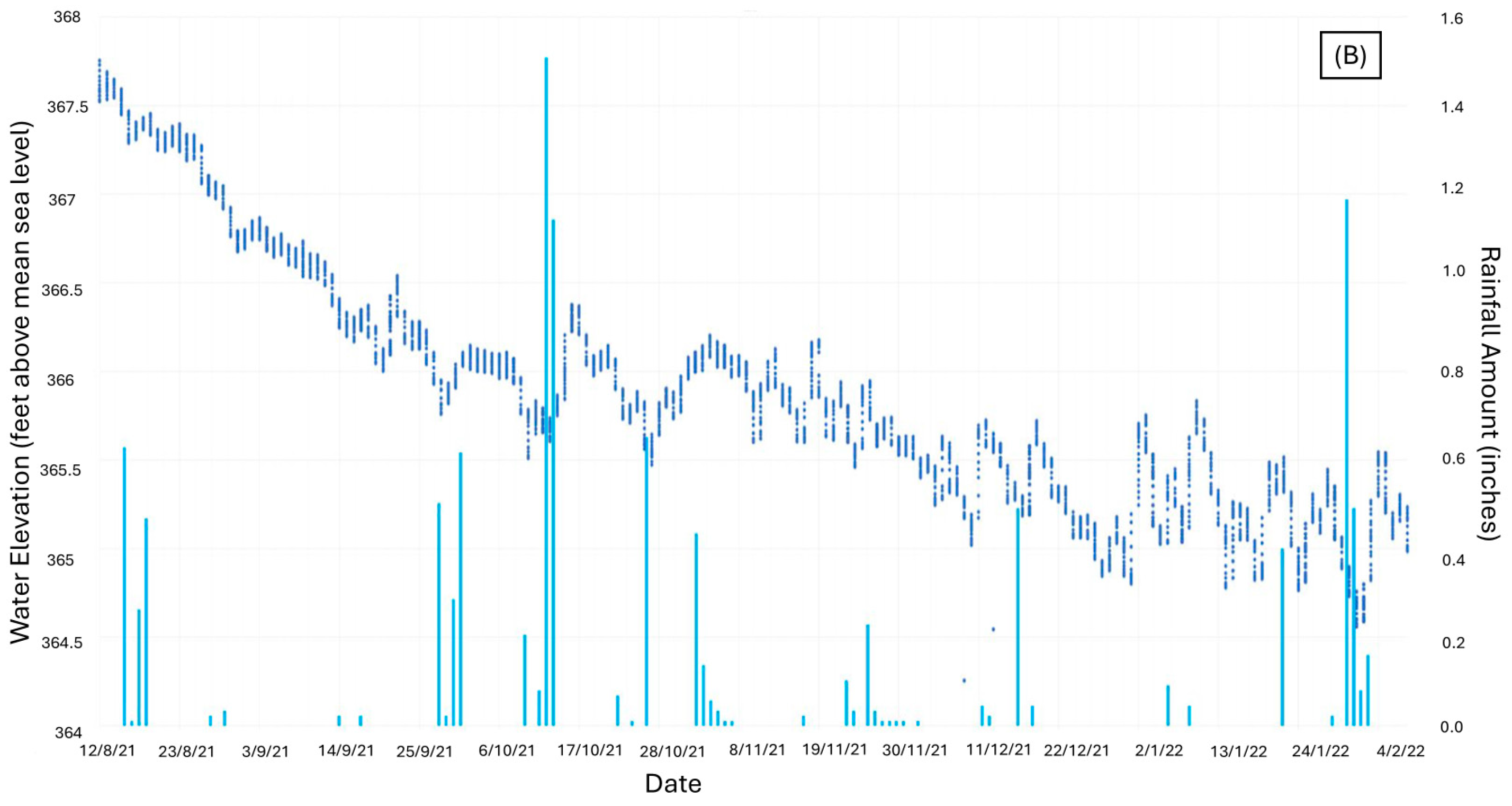However, when examined hourly, trends are more evident (Figure 7).

With the hourly groundwater data plotted against rainfall, it is possible to see the rapid increases in water level in the aquifer in response to rain events; however, these rises are frequently attenuated. Water levels return to previous trend levels quickly after the cessation of rain. This could indicate that rebound effects from pumping decrease during rain events (as mentioned above) rather than true recharge. Even with hourly data, the trend for the groundwater levels is decreasing over the course of the monitoring period as shown in Figure 6.

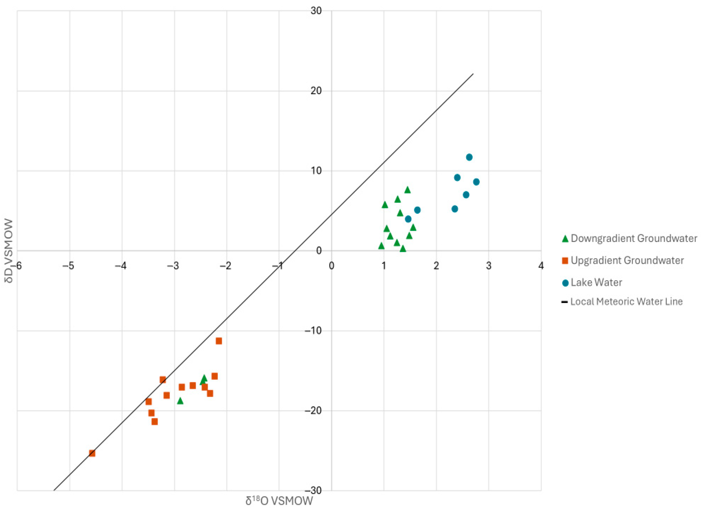
¹⁸O and ²H isotopes samples are plotted for both lakes and their respective piezometers in Figure 8. The isotopes in most piezometers and between the lakes support the notion that the lakes are flow-through systems with the lakes showing the greatest amount of evaporation-driven change in their isotope ratios between all measurements; plotting farthest from the local meteoric water line from data gathered in Waco, Texas [28], the upgradient measurements show the least evaporation effects and plot most similarly to the precipitation values. The downgradient samples plot intermediately, signifying the influence of the lake/atmospheric exposure on the isotopic signature of the water flowing along the lake flow path in the aquifer. For ¹⁸O and ²H isotopes, evaporation of the sampled water is exhibited in a proliferation of heavier isotopes as lighter ones selectively evaporate first. In comparison to the local meteoric water line, this means waters that have undergone evaporation after rainfall plot either above or to the right of the line (depending on the primary enriched heavier isotope).

In this area, the upgradient groundwater samples plot primarily as rainwater as the water that enters the aquifer system does not have time to evaporate under atmospheric conditions. In Figure 8, it is possible to see some locations where the data do not follow the trend. The downgradient measurements that plot with the upgradient measurements are sourced from ES2 and ES3 at the East Site. These piezometers were constructed with maximum depths deeper than the bottom of the gravel pit lake. It is likely that these isotope samples are indicative of a deeper flow path in the aquifer that does not intersect the flow path that provides water to the lake, like the deeper flow paths that McVea [15] found in his modeling efforts in the BRAA. The lake samples that plot closer to the downgradient measurements may have been a result of those samples being taken in the month of May, before the high temperatures and dryness of the following months began. This would lead to less evaporation than may have been evident had the samples been taken in the following months of the summer.

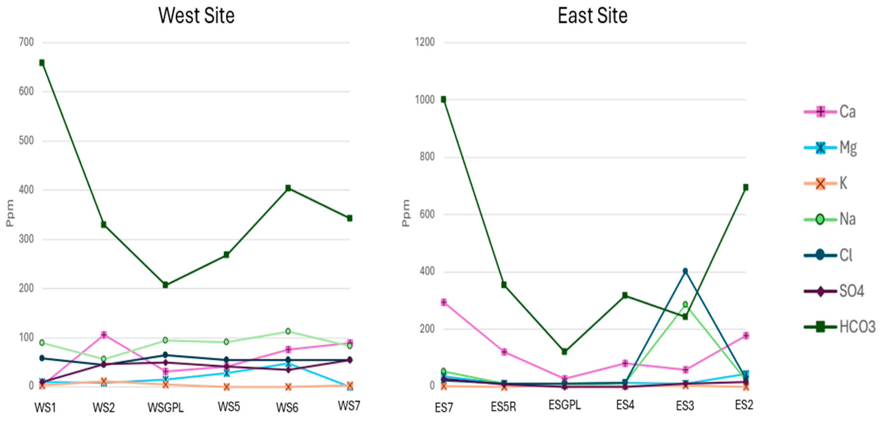
Cations and anions stay relatively consistent as the water flows from upgradient piezometers through the lake to downgradient piezometers (Figure 9).

The notable exception to this is HCO₃, which is lowest in the surface water samples from both GPLs due to the degassing of carbon dioxide as the water leaves groundwater confinement. Calcium follows HCO₃ but with less dramatic differences between groundwater and surface water; this is also due to the changes in pH from groundwater to surface water. With the increase in pH, dissolved calcite in the groundwater is reprecipitating in the lake reducing the overall amounts of HCO₃ and Ca in the water in the lakes. More conservative elements [29,30], sodium and potassium, stay consistent as water moves from groundwater to the lake and back into groundwater; this indicates the connectivity between ground and surface waters in this system.

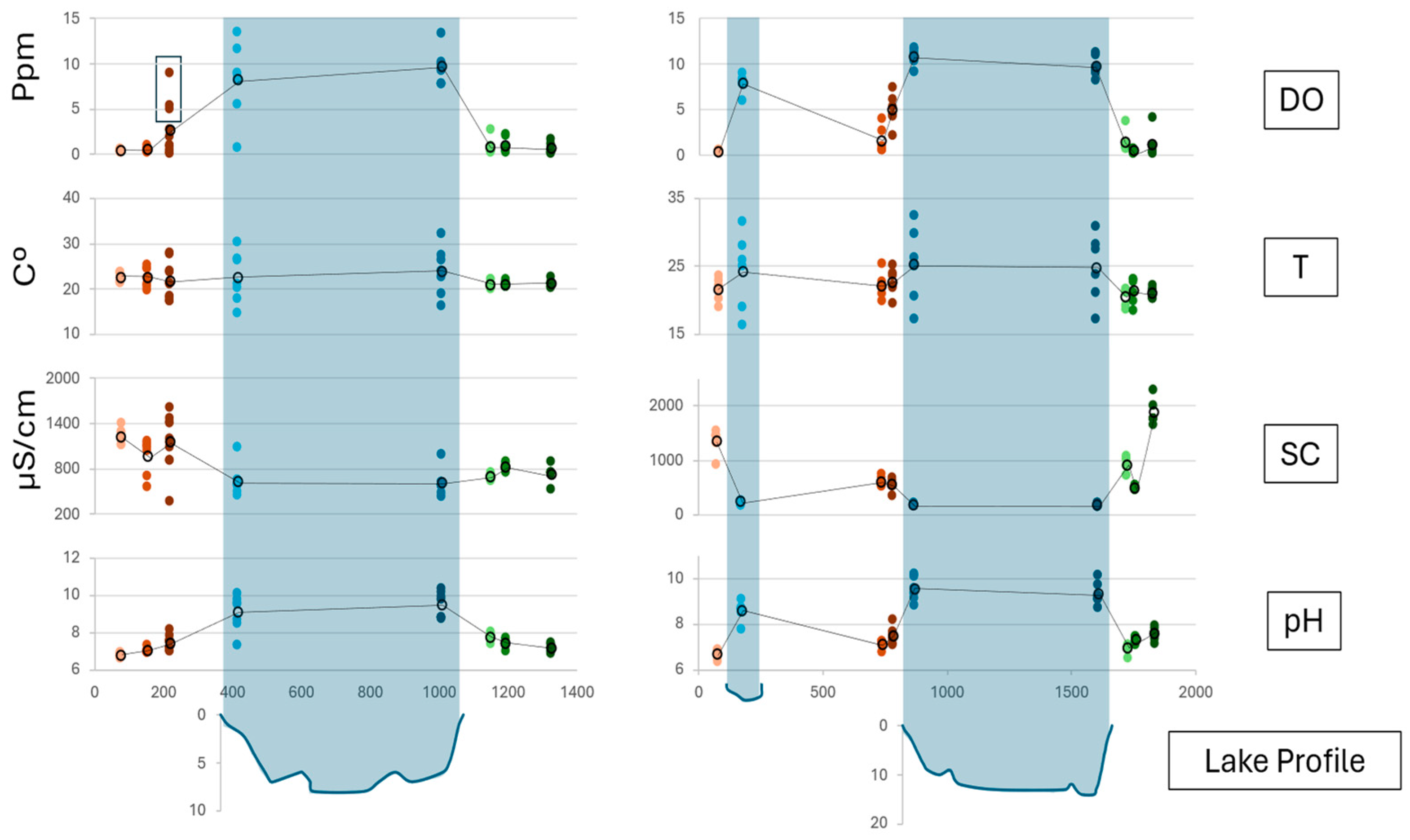
Nutrient sampling results across both lake systems also follow a distinctive pattern with some variation due to piezometer depth and the occurrence of seasonal algal blooms. Figure 10 and Figure 11 show chemistry sampling results from the piezometers and lakes for the entire sampling period.

The observed pH values show degassing effects from the water entering the surface driving the carbonate equilibria forward as CO₂. The exsolvation of CO₂ pushes the pH upwards by 1–2 units depending on the time of year (the warmer seasons appear to have a more dramatic degassing effect perhaps driven by temperature and solar irradiance). Specific conductance is consistent across the spatial dimension and the temporal dimension. Minor variation occurs between sample times and there is a relatively similar clustering of all samples in each area with the exception of the West Site’s downgradient samples which are consistent per well but differ when viewed on the whole. This is likely due to differences between the aquifer flow paths accessed by each piezometer downgradient of the West Site lake. Temperature follows the expected pattern across the sampling period. Groundwater temperatures are consistent throughout the year with minor decreases following the winter months and increases when the air temperature rises in the summer; surface water temperatures have much greater spread (a spread of +/−10 C for surface water and +/−5 C for groundwater). Dissolved oxygen patterns are also as expected with the surface water showing a much higher average DO concentration than the surrounding groundwater. Anomalously high concentrations of DO were found in multiple piezometers over the course of the study, specifically, WS3 and ES5. These piezometers were both likely cut off from the surrounding groundwater supply due to a kink and subsequent break in the casing of the well in the case of ES5 and a too shallow installation in the case of WS3. In both cases, anomalous samples were collected during the warm and dry months when the water table likely dropped below the bottom of WS3 and below the kink in ES5. These values were included and are shown in Figure 10 in a black box.

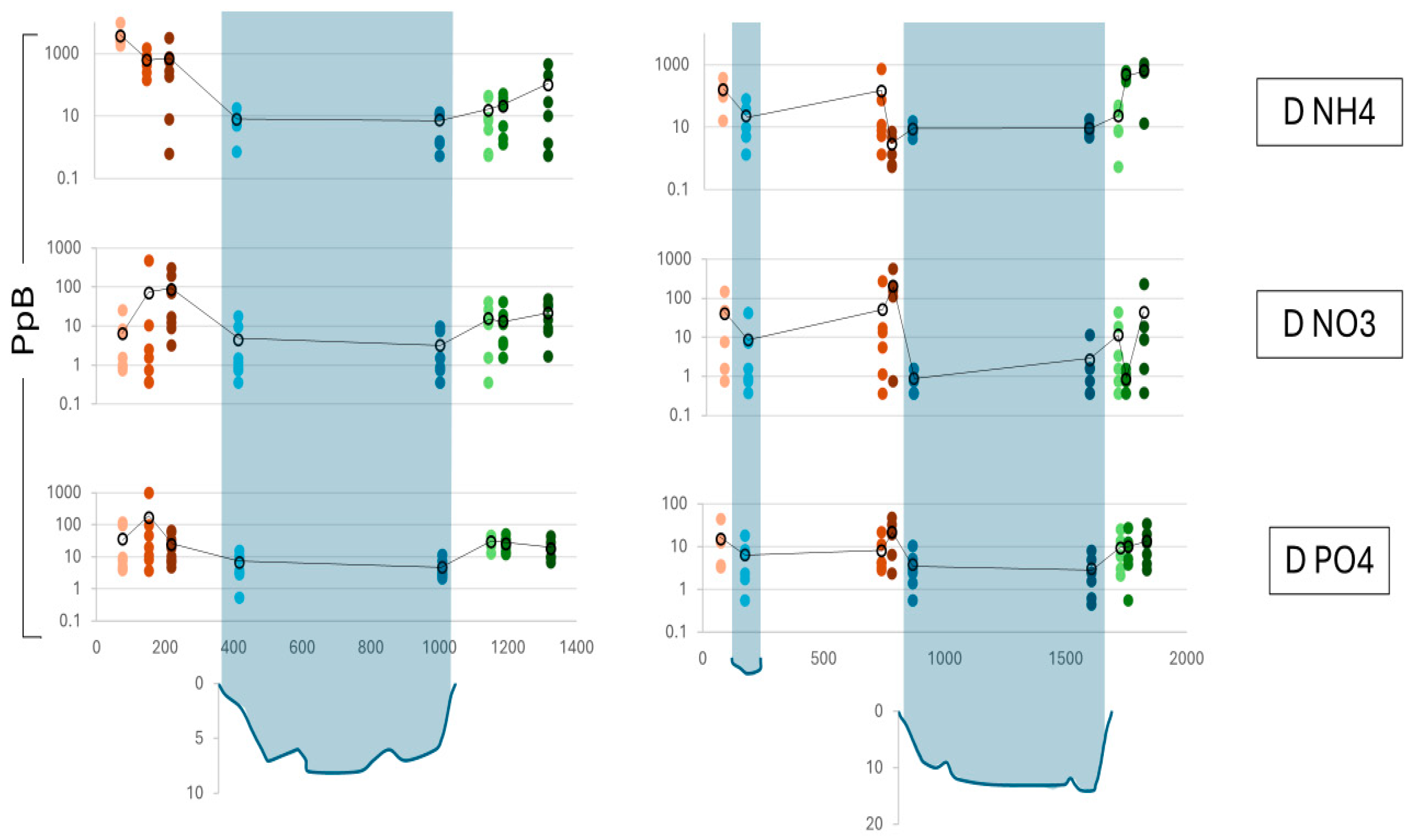
For the nutrients analyzed (dissolved phosphorus, ammonia, and nitrate), if a sample was found to be below the MDL for a given analyte, the value for that sample was reported as half the MDL for graphical and data reporting purposes. Values were considered outliers for analysis purposes if they were higher than three times the average value for all other samples. In this case, the outliers were removed from the dataset and not included. This occurred once over the course of the study and an outlier value of 6710 μg/L of dissolved nitrate was thrown out. The piezometer WS4 at the West Site showed the outlier value in the October 2021 sample run. It is possible that this piezometer was uncapped and disturbed, leading to the anomalous value. Nutrient levels decline, on average, when water enters the surface waters from groundwater. The magnitude of decline depends on surface conditions in the lake (Figure 11).

Large algal blooms occurred in both lakes over the summer of 2021 which died off in the winter and regrew partially in the spring of 2022. These blooms are an influence on nutrient consumption and production in the lakes as has been shown in other lakes [31,32]. Many of the samples with the lowest observed nutrient levels are during these time periods. Clustered samples from downgradient, lakes, and upgradient piezometers suggest the remediation of nutrient contamination like that shown in similar work [7,11]. However, it must be acknowledged that the systems examined in those projects were quite different from the lakes described in this paper. Those lakes were deeper, more distinctly connected to the groundwater system, older, and larger. It is likely that lakes in this more shallow, alluvial system function differently depending on pre-existing conditions and are more responsive to changes in general conditions (rainfall) and wildlife disturbance. However, the prevalence of lakes like the ones examined in this project within the alluvial aquifers of Texas (and the continued expansion in their numbers), and the lack of regulation regarding their construction and use, means that their effects could be compounding quickly.

According to the chemical analyses, the two GPLs studied appeared to be flow-through systems throughout the studied period. However, both lakes were especially close to the Brazos River. In this area, groundwater discharges into the river indicating a steeper groundwater gradient when compared to other sections of the aquifer that are farther from the river. Lakes farther from the river would likely have different dynamics and would require further investigation as to their effects on the aquifer. It is possible that they may behave more as evaporative sinks in late summer or other extended dry periods (which will increase in potency and length moving into the next 25 years of Texas climate [17]). Less flow through the lakes could also affect their potential to remediate nutrients or reverse their effects through “evapo-concentration”, causing them to behave as sources of increased nutrients rather than as remediation sites.

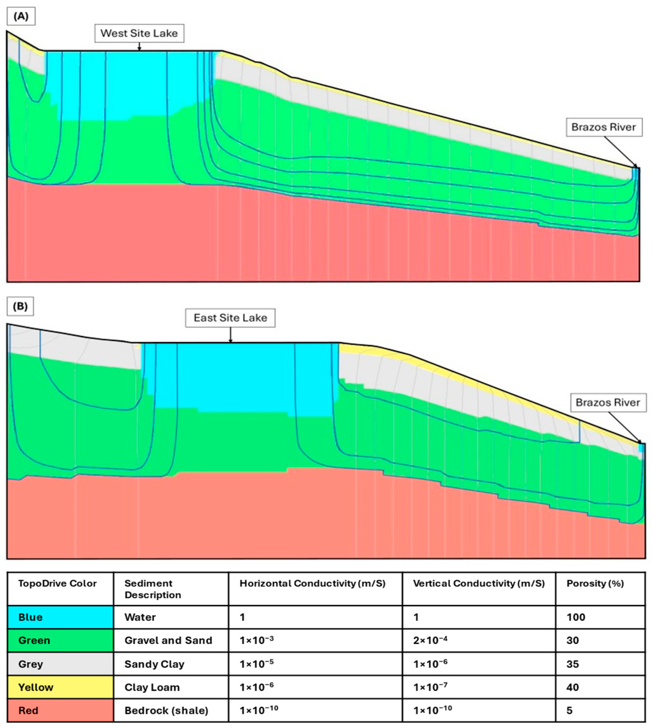
To the authors’ knowledge, the evaporative groundwater loss from GPLs or similar groundwater-fed anthropogenic water features is not considered in any groundwater availability models [25] or official water budgets for the BRAA. The exploratory modeled flow paths from the TopoDrive model using specific local lithology from the piezometers at each site (Figure 5) suggest again that water flows into each lake from the upgradient side of the lake and exits it from the downgradient side of the lake and that the deeper parts of the lake see a higher volume of groundwater inflow than do the banks [26]. At both sites, the downgradient flow paths saw, on average, an order of magnitude increase in the speed that a particle of water would travel in a day (0.87 ft/day upgradient vs. 12.6 ft/day downgradient at the West Site and 2.9 ft/day upgradient vs. 9.2 ft/day downgradient at the East Site) [26]. This is due to the steepening flow gradient in the direction of the river. This also means that although water is flowing into and out of the lakes at the edges, the water in the body of the lake is not experiencing significant movement. The lack of movement in the body of the lakes makes them more susceptible to surface conditions and evaporation effects.

The average total yearly evapotranspiration of the field including the East Site lake (for the period of record, 2019–present) is just over 38 inches per year [33,34]; this number is mediated by the grassy shoreline being included in the estimate. Although an open water calculation was used, the actual pure evaporation for just the lake surface may be a larger value. The average rainfall for the greater Waco area is around 32 inches per year (for the same period of record) [35]. The difference of six inches per year over the 10-acre lake is equivalent to an average loss of 5 acre-feet per year or 1.63 million gallons per year. This means that this lake is the equivalent of a well pumping at three gallons per minute 24 h per day, 365 days per year. In other terms, the evaporative loss from this lake is equivalent to the daily household water use of 20 single family homes for a year (an average use of 220 gallons per day) [36]. It is conceivable that lakes of similar sizes in the Waco area would produce similar evaporative patterns and result in an overall and continual decrease in water levels within the aquifer particularly during drier years. As of 2014, 4100 acres of the BRAA in McLennan County had been subject to gravel pit mining with no remediation [37]. Using the six-inch difference in rainfall and lake evaporation in the previous paragraph, the evaporative loss of all the 2014 open GPLs would be 2050 acre-feet of water per year, or the equivalent water use of 8300 single family households in Texas. Although some of these lakes have likely been partially backfilled or altered to enhance them aesthetically and some lakes have likely been remediated since 2014, the overall number of lakes has increased [1]. Increasing the lake surface area will yield increasing ET losses to the aquifer water supply and therefore could also affect the baseflow of the Brazos River itself. The presence or absence of such effects should be examined and quantified before any future policy adjustments are considered to account for GPLs or further water well drilling. While parallels can be drawn between the evaporative loss of water from GPLs and the losses from the aquifer due to irrigation, irrigation provides some return flow to the aquifer and is more seasonal. Evaporative loss from the surface of the GPLs might slow in the winter but, due to the Texas climate, it is continuous throughout the year and can be a considered a complete loss of water from the system as the lakes are not large enough to influence cloud formation or general humidity in the area. The estimated water use for agricultural irrigation in McLennan County is around 3500 acre-feet per year as of 2013 [38]. Water used for irrigation is not totally lost due to evapotranspiration, as there is return flow to the aquifer; however, this can be difficult to quantify, and a large fraction of water pumped for irrigation will be lost to evapotranspiration. The total evaporative loss of water from the lakes is 58% of all the water used for irrigation in the county, making it a significant and underreported source of water loss in the BRAA.

4. Conclusions

Further monitoring and expansion of our understanding of how these anthropogenic ecosystems affect groundwater quality is necessary; however, it is clear that they can function as flow-through systems under the right conditions and serve as potential areas of remediation for nutrients commonly used in the BRAA, improving overall water quality at the expense of serving as sites of high evaporative loss, essentially being wells with surface areas of multiple thousands of feet squared. Using satellite-based evapotranspiration data led to suspected losses of hundreds of millions of gallons of water over the course of the observation period in this study [33,34]. Trading water quality for water quantity in this aquifer may be detrimental for the long-term health of the water supply from the deeper flow paths, and the continued construction of GPLs may exponentially increase the evaporative losses to the point where any improvement in water quality is rendered moot.

Overall, this study does not manage to address the aggregate effects of all gravel pit lakes on the BRAA due to disparities between individual lakes, including proximity to the river and thus the groundwater gradient, the land use surrounding the lake, and the legacy and history of the lake and its age. Future work in similar GPL–groundwater systems should attempt to account for these differences by increasing the number of studied lakes, and studying lakes with more geographic variability, with a specific emphasis on lakes further from the river and in thicker aquifer sections with less compartmentalization.

The effects of GPLs will also continue to shift as the move towards urbanization continues; this makes it difficult to predict how the lakes will affect the aquifer moving forward, especially considering the lack of characterization of the lakes previously. This study highlights that the lakes are experiencing groundwater and surface water interaction as evidenced by shifts in water chemistry as water flows from groundwater to the lakes and back to the aquifer. The study attempts to examine the shape that such interactions take, which is important when considering the future impacts that the continuous construction of more such lakes will have.