Abstract
Exploratory structural equation modeling (ESEM) allows items to cross-load on nontarget factors and provides flexibility in modeling multidimensional survey data. However, this flexibility comes at the cost of increased model complexity due to the estimation of a significantly greater number of parameters than conventional SEM. This study systematically evaluated the model fit indices in ESEM through a Monte Carlo simulation. Design factors included model complexity,atent factor correlations, magnitudes and percentages of major cross-loadings, and sample sizes. Results showed that both the number ofatent factors m and the item–factor ratio p/m had distinct impacts on rejection rates, particularly in underspecified models. Among the fit measures, tests and Mc demonstrated high power for detecting misspecification while, in general, elevating false positives. CFI and TLI provided a more balanced trade-off between false- and true-positive rates. When evaluating ESEM, it is important to consider multiple fit indices and justify the cutoff criteria across models with different factor structures.
1. Introduction
Measurement constructs in psychology, education, and the social sciences are often multidimensional and rarely follow a simple structure in which each itemoads on only oneatent factor (McDonald, 1985). In factor analysis, the common practice of ignoring minor cross-loadings (Cudeck & O’Dell, 1994) to achieve a simple structure can deteriorate the model fit and result in biased parameter estimates (Marsh et al., 2011). Exploratory structural equation modeling (ESEM; Asparouhov & Muthén, 2009) allows items to cross-load on nontarget factors and provides flexibility in modeling multidimensional survey data. ESEM has been frequently used in empirical research to improve model fit and avoid inflation of factor correlations (Marsh et al., 2010; Morin & Maïano, 2011). As ESEM estimates all potential factoroadings (including primaryoadings and cross-loadings) in the exploratory part of the model, it estimates a significantly greater number of parameters and thus markedly increases model complexity compared to the conventional SEM. Model complexity has been shown to affect the fit indices in conventional SEM (Shi et al., 2019), whereas it is not clear whether the commonly used fit measures are appropriate for evaluating the fit of ESEM models. This issue was also raised in Marsh et al. (2009), who suggested that more research is necessary to evaluate the behavior of the fit indices in ESEM. In practice, researchers often use the conventional cutoff criteria developed for SEM (Hu & Bentler, 1999) to evaluate the model fit of ESEM. However, the applicability of these fit criteria for ESEM remains unclear. It is not yet established how to best interpret model fit in ESEM and whether existing criteria can be applied broadly or only selectively to certain indices. Thus, this study aims to examine the performance of commonly used fit indices in model evaluation for correctly and misspecified ESEM models across varyingevels of model complexity, cross-loading conditions, and sample sizes.
1.1. Exploratory Structural Equation Modeling
ESEM has been widely applied for validating psychological measurement instruments where strict simple structure assumptions are unrealistic. Common applications include personality inventories (e.g., validating the structure of the Big Five personality traits; Marsh et al., 2010), motivational scales (e.g., examining intrinsic and extrinsic motivation dimensions; Howard et al., 2018), and clinical assessments (e.g., modeling symptom overlap in psychopathology measures; Caci et al., 2015). In these applications, theoretically distinct constructs exhibit empirical overlap due to shared variance, method effects, or construct complexity. Traditional CFA methods that impose strict simple structure are often overly restrictive in such cases, making ESEM a more appropriate alternative.
An ESEM model may consist of exploratory, confirmatory, or both components. The confirmatory component typically assumes a clear factor structure specified a priori based on theory and is estimated using the parameterization of the confirmatory factor analysis (CFA; Jöreskog, 1969). The exploratory component can be divided into blocks that contain different sets of factors and estimated using an exploratory factor analysis (EFA; Jennrich & Sampson, 1966). The ESEM follows the framework of conventional SEM, while allowing for a set ofatent factors to be exploratory, with all cross-loadings freely estimated. The measurement model (Equation (1)) and structural model (Equation (2)) of ESEM can be expressed, respectively, as follows:
where is a vector of indicators (e.g., survey items), is a vector of item intercepts, is a matrix of factoroadings, is an vector of factor scores, is a matrix of coefficients regressing on , is a vector of covariates, is a vector of measurement errors, is an vector of factor intercepts, is an matrix of structural coefficients among , is an matrix of structural coefficients regressing on , and is an vector of factor disturbances. Measurement errors and factor disturbances are assumed as and , respectively, where and are typically constrained to be diagonal, although allowing for correlated residuals represents a more flexible scenario in practice.
Theatent factors can be grouped into CFA or EFA factors, estimated in the same model simultaneously. Multiple blocks can be used for the EFA factors. Within a block, all itemsoad on all EFA factors in that block. The same relationship should be specified between all EFA factors within the same block and factors/covariates outside of the block. To estimate the EFA component, an initial or unrotated solution is first derived using maximumikelihood (ML) estimation, and then a rotation (e.g., Quartimin, Geomin, target) can be applied to yield a more interpretable factor structure if needed (Asparouhov & Muthén, 2009). At the initial step, a total of constraints are imposed for identification purpose, where m is the number of factors. The factor covariance matrix is given as constraints for the unique elements, and the factoroading matrix is given as constraints, adding up to .
For the EFA blocks, the number of factors is determined in an exploratory manner, similar to traditional EFA. A set of candidate models with varying numbers ofatent factors are estimated and compared, and the model demonstrating the best fit based on established evaluation criteria is selected for inclusion. Thus, it is critical to understand the strengths andimitations of common fit indices, such as the comparative fit index (CFI; Bentler, 1990), Tucker–Lewis index (TLI; Tucker & Lewis, 1973), and root mean square error of approximation (RMSEA; Steiger & Lind, 1980), in guiding the evaluation of EFA factor structures. More details of SEM fit indices will be introduced in the next section.
1.2. Goodness-of-Fit Indices
Goodness-of-fit indices, including CFI, TLI, RMSEA, McDonald’s centrality index (Mc; McDonald, 1989), gamma hat (GH or ; Steiger, 1989), and standardized root mean square residual (SRMR; Bentler, 1995), are commonly used to quantify the degree of agreement between a hypothesized model and the observed data. The computational formulas for a set of widely used fit indices are presented as follows:
In Equations (3)–(8), T is the chi-square statistic, the subscripts T and B indicate the target and baseline models, N is the sample size, p is the number of items, s is the observed variance or covariance, and is the reproduced variance or covariance.
All the indices above but SRMR are a function of df, an indicator of model complexity. In ESEM, as the number of free parameters is considerably great, the df would be markedlyower than in conventional SEM. The df is compared with the chi-square statistic T via either the ratio or the difference in the calculation of these fit indices. As both the T and df tend to decrease in ESEM, it is unknown whether general guidelines (Hu & Bentler, 1999) for applying these fit indices are appropriate in ESEM. In addition, the number of items and the sample size also play a role in calculating the fit indices, but their impact on the fit indices in ESEM requires further investigation.
1.3. Impact of Model Complexity
The impact of model complexity on fit indices in SEM was typically examined for (1) correctly specified models, where increasing the number of indicators often results in a decline in model fit suggested by chi-square tests, CFI, and RMSEA, and (2) misspecified models, where additional observed variables sometimes increase the power of detecting model misspecification. Simulation studies (e.g., Ding et al., 1995; Marsh et al., 1998) demonstrated thatarger numbers of indicators can inflate the chi-square statistic and bias other fit indices, particularly in small samples. Similarly, Breivik and Olsson (2001) and Kenny and McCoach (2003) showed that RMSEA tends to improve artificially with more observed variables regardless of model misspecification, whereas CFI is somewhatess sensitive, though it can decrease under certain conditions. These findings highlight the nuanced relationship between model complexity and the behavior of fit indices.
The model complexity can be characterized in multiple ways, including the number of items (p), ratio of items to factors , the number of free parameters (q), and the degrees of freedom (df). Model size can be viewed as a component of model complexity. Specifically, model size refers to structural complexity, such as the number of items andatent variables. Model complexity more broadly encompasses structural complexity along with parametric complexity (e.g., number of freely estimated parameters) and constraint complexity (e.g., equality constraints, fixed vs. free parameters). Most research has emphasized the number of observed variables as the dominant driver of model size effects (Fan & Sivo, 2007; Kenny & McCoach, 2003; Moshagen, 2012), while Shi et al. (2018, 2019) extended this work to show that both the number of items p and the number of free parameters q can influence fit indices. Specifically, p and q are two important determinants of theikelihood ratio tests (Shi et al., 2018, 2019), and p also has a differential impact on CFI, TLI, and RMSEA. In addition, in the measurement invariance context, where constrained invariance models can be viewed as a type of model misspecification, Cao and Liang (2022b) found that CFI and RMSEA failed to detectoading noninvariance witharge model sizes (e.g., 6 factors, 8 items each), while chi-square-basedikelihood ratio tests were minimally affected.
Building on these findings, the present study considers the number ofatent factors m and the number of items per factor as the indicators for model size, providing a framework to evaluate how fit indices perform under differentevels of complexity in ESEM. In addition, incorporating all potential cross-loadings in ESEM substantially increases model complexity (q increases and df decreases) compared to conventional SEM. Given the unique specification of ESEM, which introduces additional parameters through the estimation of cross-loadings, the generalizability of fit measures in ESEM warrants systematic investigation.
1.4. The Current Study
Research in ESEM has spanned several areas of focus, including comparisons between ESEM and traditional CFA andatent regression using frequentist estimation (Mai et al., 2018; Marsh et al., 2020), evaluations of ESEM and Bayesian SEM in handling cross-loadings (Guo et al., 2019; Liang et al., 2020; Xiao et al., 2019), assessments of the behavior of ESEM and CFA fit indices (Konold & Sanders, 2024), investigations of composite reliability in ESEM and CFA (Fu et al., 2022), and testing of measurement invariance (Cao & Liang, 2022a). Yang and Xia (2015) examined the use of ESEM for determining the number of factors in ordered categorical data, focusing on the performance of LRT, RMSEA, and weighted root mean square residual (WRMR; Yu, 2002) under correctly specified, underspecified, and overspecified models. However, their study design was restricted to three-factor models, a limited set of cross-loading structures, and a small selection of fit indices. Prior research has demonstrated that model size can exert a pronounced impact on fit indices (Cao & Liang, 2022b; Shi et al., 2018, 2019). For instance, RMSEA tends to decrease as the number of indicators p increases; CFI, TLI, and RMSEA suggest a poorer fit with smaller N,arger p, and weaker factoroadings. Importantly, as most fit indices were originally developed and calibrated within CFA or SEM models that impose more restrictive constraints, their performance may not generalize directly to the more flexible structure of ESEM.
Thus, examining ESEM under varying model sizes is essential for understanding the behavior of fit indices. Moreover, most prior studies have primarily focused on CFI, TLI, and RMSEA. The present study extends the work by including a broader range of fit indices, whose performance in ESEM under increasing model complexity and various cross-loading patterns has yet to be systematically examined. Investigations of fit indices in ESEM provide guidance on how they should be interpreted when selecting factor structures or testing theoretical models. In our study, the correctly specified, underspecified, and overspecified models were investigated under various conditions, including model complexity, cross-loading patterns, and sample sizes. In the next section, we detail the choice of conditions and criteria used for outcome evaluation in the simulation study.
2. Method
2.1. Population Models
2.1.1. Model Size
Model size has been shown to influence the fit indices in SEM (Shi et al., 2019). In a review of factor analysis studies by Henson and Roberts (2006), the typical number ofatent factors extracted ranged from one to seven, and the number of measured items ranged from 5 to 110. We thus examined models with fourevels of complexity: 3 factors with 5 items each (F3,I5), 3 factors with 10 items each (F3,I10), 6 factors with 5 items each (F6,I5), and 6 factors with 10 items each (F6,I10). All items were continuous, multivariate, and normally distributed. The primaryoadings were all set at 0.70, and the item residual variances were set at 0.50. Latent factors followed a standard normal distribution. The factor correlations were set at 0.30 and 0.80, representing relatively small andarge correlations amongatent factors.
2.1.2. Cross-Loadings
In ESEM, all possible cross-loadings are model parameters, and the size and percentage of cross-loadings may have an impact on the model fit evaluation. In the present study, the cross-loadings were classified into major cross-loadings and minor cross-loadings. For major cross-loadings, the loading magnitudes were set to 0.15 and 0.30, and the percentages were 20% and 40% of all items, which is inine with previous ESEM research (Guo et al., 2019). The major cross-loadings were evenly distributed acrossatent factors. For instance, for the model with 3 factors and 15 items in total, 20% of the 15 itemsed to three major cross-loadings on the 3 factors, respectively. The rest of the cross-loadings in the factoroading matrix were minor cross-loadings, generated from a normal distribution (0, 0.05) (95% CI: [−0.10, 0.10]) andimited within ±0.10. That is, if the generated value for a minor cross-loading went beyond ±0.10, we discarded this value and re-generated a value from (0, 0.05) until it was within ±0.10. This specification ensured that all cross-loadings fell within the interval [−0.10, 0.10] and were negligible in magnitude, which is consistent with empirical findings showing that most cross-loadings in psychological measures are small but non-zero (e.g., Asparouhov & Muthén, 2009; Tóth-Király et al., 2017).
2.1.3. Sample Sizes
Five sample sizes were considered: 100, 200, 500, 1000, and 2000. As a result, the ratios of the sample size over the number of items ranged from 1.67 to 133.33. Since ESEM has been applied to assessarge-scale data (Marsh et al., 2009), includingarge sample sizes allows for the investigation of the robustness of the fit measures toarge samples. On the other hand, small sample sizes are common in practice and have been a focus of prior research; therefore, they were both included.
Fully crossing all design factors, the total number of data generation conditions was 160: 4evels of model complexity × 2 factor correlations × 5 sample sizes × 2 magnitudes of major cross-loadings × 2 percentages of major cross-loadings.
2.2. Data Analysis
For each condition, we generated 1000 datasets for analysis. Mplus 8.4 and SAS 9.4 were used to generate and analyze the data. For the three-factor models (F3,I5 and F3,I10), we estimated four ESEM models with 1 factor (underspecified), 2 factors (underspecified), 3 factors (correct specification), and 4 factors (overspecified). For the six-factor models (F6,I5 and F6,I10), we estimated four models with 2 factors (underspecified), 4 factors (underspecified), 6 factors (correct specification), and 8 factors (overspecified). It is to note that the ESEM analysis models specify that all itemsoad on every factor and do not differentiate between primary and cross-loadings. The misspecifications arose from the number of factors specified rather than from the specification of theoading matrix. For identification purpose, eachatent factor’s mean and variance were fixed to zero and one, respectively.
Models were analyzed using MLE with the Geomin oblique rotation. The constant added to the Geomin function in Mplus was set to 0.001 to produce minimal bias of estimation (Asparouhov & Muthén, 2009). In ESEM, items wereoaded on their main factors, whereas cross-loadings were “targeted”, but not forced, to be as close to zero as possible with the oblique target rotation procedure (Browne, 2001). Geomin has become increasingly recognized as a strong default choice for oblique rotation in factor analysis. It is noted that alternative rotation methods may affect the rotatedoading pattern but not the fit indices. Across reasonable oblique rotations, the overall fit and broad factor structure are typically stable (Asparouhov & Muthén, 2009). The number of data analysis conditions was 640 (160 population conditions × 4 analysis models).
2.3. Outcome Evaluation
For each analysis condition, the convergence rates were first examined. We then conducted an analysis of variance on the rejection rates of fit indices across the eight analysis models to assess the relative contribution of design factors in the simulation. Subsequently, we evaluated model rejection rates based on the chi-square tests at the 0.05 alphaevel, along with commonly applied fit index cutoff criteria for inadequate model fit: CFI < 0.95, TLI < 0.95, RMSEA > 0.06, Mc < 0.90, Gamma hat < 0.90, and SRMR > 0.06 (Hu & Bentler, 1999). The rejection rate was defined as the proportion of replications in each condition in which a model was flagged as exhibiting inadequate fit by a given index. These rejection rates represent false-positive (FP) rates for correctly specified models, while true-positive (TP) rates are for misspecified models.
3. Results
3.1. Analysis of Variances
All conditions achieved 100% convergence rates, including the most complex model (F6,I10) with the smallest sample size ().
Table 1 shows the eta-squared of each design facet and their two-way and three-way interactions on explaining the rejection rates of fit indices in three-factor scenarios. Design facets showing ateast a small effect size ( 0.01; Cohen, 1988) were identified as salient and are summarized in Table 1. When the three-factor model was underspecified to be one factor, sample size, number of items, the magnitude of factor correlations, as well as all four two-way interactions and the three-way interaction had an eta-squared higher than 0.01 for the rejection rates of chi-square, CFI, TLI, RMSEA, and Mc. The three-way interaction between N, p, and latent correlation revealed that the effects of sample size on fit measures were not identical across all combinations of item number andatent correlation. For example, the improved power ofarger sample sizes was compromised with an increasing number of items and a higheratent correlation for CFI in severe model misspecification. This three-way interaction suggests that recommendations for fit measures cannot be made based on the single design factor, but rather should consider the joint effect of sample size, model size, and latent relationship between constructs. For GH, only the number of items, the magnitude of factor correlations, as well as the interaction between the number of items and the magnitude of factor correlations were identified. For SRMR, the eta-squared of the magnitude of correlations was dominant at 0.93, and sample size was also salient. When the model was underspecified to be a two-factor model, the eta-squared of the magnitude of factor correlations became more salient for all the fit indices, especially RMSEA, GH, and SRMR. When the model was correctly specified to be a three-factor model, the FP rates majorly depended on sample size, number of items, and the interaction between sample size and the number of items. The rejection rates of SRMR had zero variability, so the ANOVA results could not be obtained. When the model was over specified to be a four-factor model, the pattern of the design factors was similar to the correctly specified model.

Table 1.
ANOVA for three-factor models.
Table 2 shows the eta-squared of each design facet and their two-way and three-way interactions on explaining the rejection rates of fit indices in six-factor scenarios. When the model was underspecified, the pattern of eta-squared of the design facets was similar to that of the three-factor model. On the other hand, when the model was correctly specified or overspecified, only sample size, number of items, as well as their interaction were salient, which was different from the three-factor model.
Table 2.
ANOVA for six-factor models.
3.2. False-Positive Rates
Figure 1 and Figure 2 present the false-positive rates for correctly specified models. When the model was correctly specified, the FP rates of the fit indices rejecting the model using the criteria discussed above depended on sample size and model size, except SRMR, which was zero in all conditions. With F3,I5 conditions, when the sample size was 500 and above, the FP rates of all fit indices were zero, regardless of the magnitude of correlations between the factors, except chi-square, which was around 0.05. When sample size was at 100 and the factor correlation was 0.30, the FP rates of chi-square, CFI, TLI, RMSEA, and Mc ranged from 0.12 to 0.15, 0.03 to 0.05, 0.13 to 0.20, 0.08 to 0.11, and 0.10 to 0.13, respectively. GH and SRMR had FP rates of zero in all conditions. When the sample size increased to 200, the FP rates of chi-square, TLI, RMSEA, and Mc decreased as shown in Figure 1. When the correlation among factors were 0.80 (see Figure 2), the FP rates of all the fit indices were generallyower compared to the correlation of 0.30, but with a similar pattern. When the model size increased to F3,I10, the FP rates of chi-square, CFI, TLI, Mc, and GH ranged from 0.05 to 0.68, 0 to 0.30, 0 to 0.46, 0 to 0.89, and 0 to 0.22, respectively. The FP rates of RMSEA were around zero in all conditions. The FP rates in the conditions of F6,I5 had similar patterns to those in the conditions of F3,I10. In theargest model size of F6,I10, when the sample size was 100, the FP rates of chi-square, CFI, TLI, Mc, and GH were all 1.00. The FP rates of RMSEA was around 0.69. When sample size increase to 500 and above, the FP rates dropped to around zero, except chi-square and Mc, which ranged from 0.07 to 0.45 and from 0.28 to 0.32, respectively. In sum, the FP rates of chi-square, CFI, TLI, Mc, and GH were inflated in smaller sample sizes, especially when the model size wasarge, and the impact of the correlations between the factors was negligible.
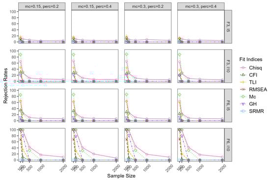
Figure 1.
False-positive rates for correctly specified models whenatent correlation = 0.30. Note: mc = magnitude of major cross-loadings; perc = percentage of major cross-loadings; F = factor; I = item.
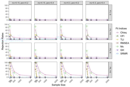
Figure 2.
False-positive rates for correctly specified models whenatent correlation = 0.80. Note: mc = magnitude of major cross-loadings; perc = percentage of major cross-loadings; F = factor; I = item.
3.3. True-Positive Rates
Figure 3, Figure 4, Figure 5 and Figure 6 show the TP rates of rejecting the underspecified model, which depended substantially on the severity of the model misspecification. For example, when the three-factor and six-factor model were misspecified to be one-factor and two-factor models, respectively, the severity of misspecification was more severe than being misspecified to be two-factor and four-factor models, respectively. Also, the under-misspecification of the ESEM models with 0.30 correlations among the factors was more severe than with 0.80 correlations among the factors. In the F3,I5 conditions with correlations among the factors of 0.30, when the three-factor model was specified to be a one-factor model, the TP rates were almost all 1.00 for all the fit indices, regardless of the design facets. This pattern was also observed witharger model sizes.
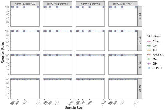
Figure 3.
True-positive rates for severe underspecified models whenatent correlation = 0.30. Note: mc = magnitude of major cross-loadings; perc = percentage of major cross-loadings; F = factor; I = item.
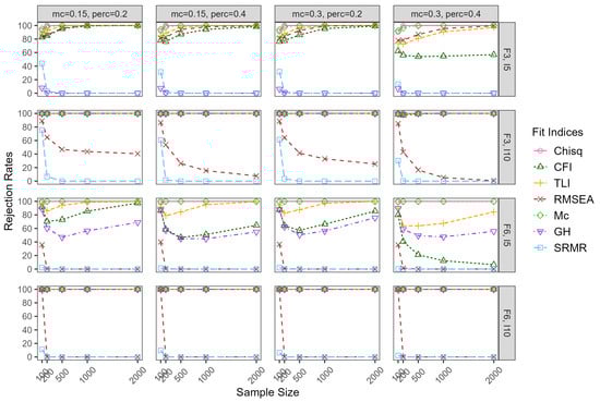
Figure 4.
True-positive rates for severe underspecified models whenatent correlation = 0.80. Note: mc = magnitude of major cross-loadings; perc = percentage of major cross-loadings; F = factor; I = item.
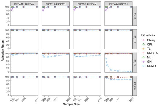
Figure 5.
True-positive rates for mild underspecified models whenatent correlation = 0.30. Note: mc = magnitude of major cross-loadings; perc = percentage of major cross-loadings; F = factor; I = item.
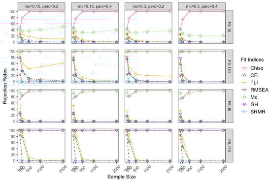
Figure 6.
True-positive rates for mild underspecified models whenatent correlation = 0.80. Note: mc = magnitude of major cross-loadings; perc = percentage of major cross-loadings; F = factor; I = item.
When the correlations among the factors were 0.80 in F3,I5 conditions, TP rates of chi-square, CFI, TLI, RMSEA, and Mc ranged from 0.91 to 1.00, 0.55 to 1.00, 0.73 to 1.00, 0.78 to 1.00, and 0.94 to 1.00, respectively. Note that CFI appeared to be the only fit index that was impacted by the percentage and magnitude of cross-loadings, with lower TP rates associated with more andarger cross-loadings. The TP rates of GH and SRMR were close to zero. When the model size increased to F3,I10, TP rates of chi-square, CFI, and TLI increased to around 1.00 in all conditions. However, TP rates of RMSEA decreased substantially compared to F3,I5 when the sample size wasarge, ranging from 0.01 to 0.89. The biggest change occurred to GH, increasing to 1.00 compared to around zero in F3,I5 conditions. When the model size kept increasing to F6,I5, TP rates for CFI decreased, especially when the percentage and magnitude of cross-loadings were theargest. TP rates for RMSEA decreased considerably, especially when the sample size wasarge. To be more specific, when the sample size was 500 and above, they were all zero. TP rates of GH decreased to between 0.44 and 0.90, with smaller values associated witharge sample sizes. When the model size increased to F6,I10, TP rates for all fit indices were 1.00, except RMSEA and SRMR. TP rates for RMSEA were around 1.00 in sample size of 100, but zero for all other sample sizes.
When the ESEM model misspecification wasess severe (three-factor model specified to be two-factor model, or six-factor model specified to be four-factor model) and the correlation among factors were 0.30, the FP rates of all fit indices were similar to those in the more severe model misspecification, except GH and SRMR. To be more specific, TP rates of GH wereower than they were under the more severe model misspecification when the sample size was 100. TP rates for SRMR wereower in the F6,I5 conditions, especially in the conditions with theargest percentage and magnitude of cross-loadings. SRMR was alsoower in the F6,I10 conditions with theargest percentage and magnitude of cross-loadings. However, when the correlation among the factors was 0.80 (less severe model misspecification), TP rates varied aot depending on the design facets. In the conditions of F3,I5, TP rates of chi-square increased with the sample size, reaching 1.00 when the sample size was 500 and above. TP rates of CFI, RMSEA, and TLI were around 0.40 in the smallest sample size of 100, decreasing with the sample size. TP rates of Mc were around 0.40 in all conditions, not obviously impacted by the design facets. GH and SRMR failed to detect the model misspecification. When the model sizd increased to F3,I10, the TP rates of chi-square and Mc were around 1.00 in all conditions. TP rates of TLI, CFI, and GH were around 0.80 in the smallest sample size of 100, decreasing with the increase in sample size. When the model size increased to F6,I5, the TP rates of chi-square were around 0.75 in the smallest sample size and increased to around 1.00 when sample size reached 500 and above. The TP rates of Mc dipped to around 0.80 with a sample size of 200. TLI, RMSEA, CFI, GH, and SRMR were not sensitive to the misspecification, especially when the sample size was 200 and above. In theargest model size of F6,I10, the TP rates of chi-square, Mc, and GH were all around 1.00, regardless of sample size and percentage and magnitude of cross-loadings. The remaining fit indices were sensitive to the model misspecification in the smallest sample size, decreasing dramatically to around zero with aarge sample size.
Figure 7 and Figure 8 show the TP rates for overspecified models. When the ESEM model was overspecified (three-factor model specified to be four factors, and six-factor model specified to be eight factors), the TP rates of all the fit indices had similar patterns in the two differentevels of factor correlations. Thus, only the results of the factors correlation of 0.30 were reported. All the fit indices failed to detect the model overspecification in the model size of F3,I5. When the model size increased to F3,I10 and F6,I5, TP rates of Mc were around 0.70 in the smallest sample size of 100, decreasing dramatically with the sample size. Chi-square and TLI had TP rates around 0.40 in the smallest sample size, and they dropped to around zero when the sample size reached 200 and above. The other fit indices, including CFI, RMSEA, GH, and SRMR, were not sensitive to the model over-misspecification. In theargest model size of F6,I10, chi-square, TLI, RMSE, and GH had high TP rates in the smaller sample sizes but dropped to around zero when the sample size reached 500 and above.
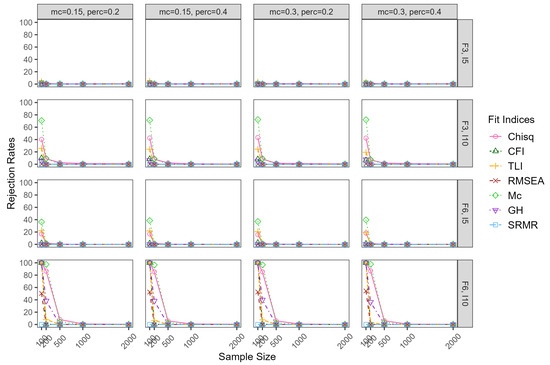
Figure 7.
True-positive rates for overspecified model whenatent correlation = 0.30. Note: mc = magnitude of major cross-loadings; perc = percentage of major cross-loadings; F = factor; I = item.
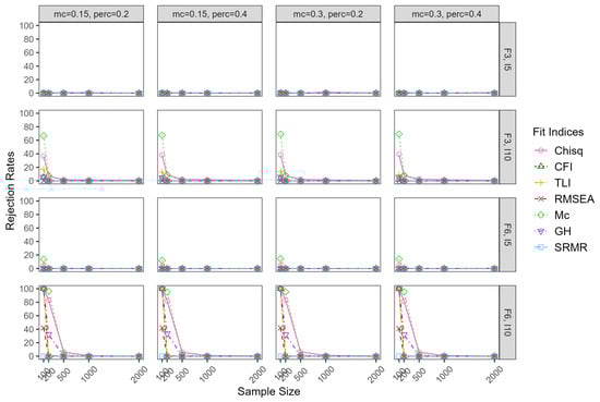
Figure 8.
True-positive rates for overspecified model whenatent correlation = 0.80. Note: mc = magnitude of major cross-loadings; perc = percentage of major cross-loadings; F = factor; I = item.
4. Discussion
This study systematically evaluated the sensitivity of fit indices to model misspecification with differentevels of model complexity and specifications within the ESEM framework. Most fit indices were developed as a function of df and fit statistic and thus can be affected by the model size and sample size to varying degrees. While ESEM provides greater flexibility than a more restrictive CFA or SEM, the additional parameters it estimates reduce the df, which may, in turn, affect the behavior of fit indices. Our study extends prior evaluation of fit indices by examining their performance in ESEM across a broader set of indices and conditions, manipulating the model size, model specification, and sample size. The findings provide researchers with empirical guidance for interpreting model fit in ESEM and contribute to a more nuanced understanding of the strengths andimitations of fit indices in applied research using ESEM.
Reconsidering the definition of model size within the ESEM framework, both the number ofatent factors m and the number of items per factor had distinct impacts on the rejection rates, especially for the underspecified models. Even when the total number of items (p) was held constant, models with feweratent factors (m) and more items per factor () tended to produce higher rejection rates for CFI, TLI, RMSEA, and GH across conditions. In contrast, rejection rates for chi-squared tests and Mc wereess sensitive to these variations. These findings are partially consistent with Shi et al. (2018, 2019), where model size effects were primarily associated with p for chi-square statistic, CFI, TLI, and RMSEA, although their focus on one-factor modelsimited insight into the role of multipleatent factors. Our study extends this work by demonstrating that the number ofatent factors m interacts with the item–factor ratio in shaping model evaluation. These results align with Cao and Liang (2022a), in which the authors found that in ESEM measurement invariance testing, when imposing increasingly restrictive constraints on model parameters—considered a type of misspecification—both p and m influenced the rejection rates of fit indices. In general, our findings suggest that multidimensional factor structures should be considered for conceptualizing model size, as it has important implications for interpreting the fit indices.
False-positive rates of fit indices were highly sensitive to model complexity and sample size, whereas the impact ofatent correlations was comparatively minimal. Chi-squared tests consistently rejected correctly specified models, while other fit indices only inflated FP rates when sample sizes were small. Increasing the model size (particularly ) inflated false positives with small sample sizes. These results concur with Shi et al. (2018), who showed that increasing p can dramatically inflate the false positives of even with a relativelyarge N. Based on their one-factor model results, they recommended to maintain acceptable FP rates. Our findings suggest that when models are multidimensional, an evenarger sample size is required to adequately control false-positive rates. Researchers should be cautious of interpreting model fit in ESEM with small samples, as spurious rejections may occur even when models are correctly specified.
The sensitivity of fit indices to underspecification is not uniform but context-dependent, affected by interactions between sample size, model size, and factor correlations. In general, chi-square tests yielded the best TP rates for underspecified models, followed by Mc; SRMR generally produced theowest TP rates. For a smallatent-factor correlation (0.3), increasing sample sizes generally increased the power of rejecting underspecified models, whereas for aargeatent correlation (0.8), the performance of fit indices showed a mixed pattern—some indices benefited fromarger samples (e.g., test, Mc), while others showed reduced sensitivity (e.g., GH, SRMR). It is noted that given the same number of misspecifiedatent factors, smalleratent correlationsed to more severe misspecification, whereasarger correlations mitigated it. Increasing generally improved TP rates except for RMSEA, which tended to beess sensitive to model underspecification inarger models. Increasing m was not guaranteed to improve TP rates for indices such as CFI, TLI, and RMSEA, which tended to decrease power when model dimensions increased. These findings were partially consistent with prior research (Breivik & Olsson, 2001; Cao & Liang, 2022a; Kenny & McCoach, 2003; Shi et al., 2019).
Overspecified models produced rejection rates similar though slightlyower than correctly specified models. This is expected, as adding an additional factor in ESEM increases flexibility and improves model fit, although the additional complexity is not theoretically justified.
4.1. Implications
The findings of the present study carry several empirical implications for ESEM applications. First, both the number ofatent factors m and the item–factor ratio influence the performance of fit indices. Caution is needed when interpreting models with different dimensionality. Two models with the same total number of items may nonetheless produce varied rejection rates depending on how items are distributed across factors. Second, the choice of fit index should be guided by the research goal. When the goal is to control false positives, neither or Mc is recommended, especially when . At sample sizes , nearly all fit indices inflated false positives, suggesting these indices areess reliable. When the goal is to detect underspecification, and Mc produced the highest power, while CFI and TLI provided a somewhat better balance between false- and true-positive rates. RMSEA, SRMR, and GH display inconsistent performance across model size, sample size, and degree of misspecification, suggesting caution in their use. However, these results were obtained using conventional SEM cutoffs, which may not be directly applicable to ESEM. It remains possible that different conclusions could emerge if more appropriate ESEM-specific thresholds were applied. Third, given the differential sensitivity of fit indices, researchers should consider multiple fit indices for model fit evaluation and take a comprehensive approach. This is important when multiple candidate models may be refitted or when studying complex psychological constructs. Fourth, practitioners should view overspecifications asess problematic, particularly in exploratory contexts, where including additional factors is preferable to omitting ones. However, it could come with the cost of more complex interpretations. Finally, the findings call for more transparency in reporting the model fit. It would be helpful to justify the cutoff criteria when comparing fit across models with different factor structures. These implications are summarized in Table 3.
Table 3.
Empirical implications for ESEM applications.
4.2. Limitations and Future Research
Severalimitations of the present study can serve as future research directions. Our evaluation of fit indices relied on conventional SEM cutoff criteria. These cutoffs are sample- and model-dependent, and using fixed cutoffs could obscure important patterns of model adequacy. Future work could explore evaluating the distribution of fit indices through permutation-based approaches (e.g., Arboretti et al., 2021) and provide suggestions based on dynamic, data-driven cutoffs (e.g., Goretzko et al., 2024; McNeish & Wolf, 2023). Moreover, the current study focused on frequentist ML estimation. Extending to estimating fit indices under the Bayesian framework would be valuable, as Bayesian methods offer advantages such as incorporating prior information, handling small sample sizes, and providing posterior distributions of fit indices (e.g., Edeh et al., 2025; Garnier-Villarreal & Jorgensen, 2020; Hoofs et al., 2018). Furthermore, our study emphasized the evaluation of single model fit over model comparison. Information criteria (e.g., AIC, BIC) would allow for a more comprehensive evaluation of the model performance, as they jointly account for model fit and complexity (e.g., Cao & Liang, 2022a; Liang et al., 2025; Liang & Luo, 2020). In addition, our study was conducted under relatively idealized conditions where all items were normally distributed for ESEM implementation. Extensions to ordinal data with robust estimation methods, such as weightedeast squares with mean and variance adjustment (WLSMV; Muthén, 1984; Muthén et al., 1997), warrant further investigation. Last, both the number of misspecified factors and the number ofatent correlations contribute to model misspecifications. Quantifying theevel of misspecifications would improve the understanding of how fit indices respond to varyingevels of model errors.
Author Contributions
Conceptualization, X.L. and C.C.; methodology, X.L., C.C. and W.-J.L.; software, X.L. and C.C.; validation, X.L., C.C. and W.-J.L.; formal analysis, X.L., C.C., J.L., E.J.E. and J.C.; investigation, X.L., C.C., J.L., E.J.E., J.C. and W.-J.L.; resources, X.L., C.C. and W.-J.L.; data curation, X.L., C.C., J.L., E.J.E. and J.C.; writing—original draft preparation, X.L. and C.C.; writing—review and editing, X.L., C.C., J.L., E.J.E., J.C. and W.-J.L.; visualization, C.C., J.L., E.J.E. and J.C.; supervision, X.L., C.C. and W.-J.L.; project administration, X.L., C.C. and W.-J.L. All authors have read and agreed to the published version of the manuscript.
Funding
This research received no external funding.
Institutional Review Board Statement
Not applicable. Computer-simulated data were used.
Informed Consent Statement
Not applicable.
Data Availability Statement
This study used simulated data. The SAS 9.4 and R 4.4.0 code for data generation and analysis is openly available at https://osf.io/njx5e/?view_only=2bb42799894e466391357e0f03476b25, accessed on 20 August 2025.
Conflicts of Interest
The authors declare no conflicts of interest.
References
- Arboretti, R., Ceccato, R., & Salmaso, L. (2021). Permutation testing for goodness-of-fit and stochastic ordering with multivariate mixed variables. Journal of Statistical Computation and Simulation, 91(5), 876–896. [Google Scholar] [CrossRef]
- Asparouhov, T., & Muthén, B. (2009). Exploratory structural equation modeling. Structural Equation Modeling: A Multidisciplinary Journal, 16(3), 397–438. [Google Scholar] [CrossRef]
- Bentler, P. M. (1990). Comparative fit indexes in structural models. Psychological Bulletin, 107(2), 238–246. [Google Scholar] [CrossRef]
- Bentler, P. M. (1995). EQS structural equations program manual. Multivariate Software. [Google Scholar]
- Breivik, E., & Olsson, U. H. (2001). Adding variables to improve model fit: The effect of model size on fit assessment in LISREL. In R. Cudeck, S. du Toit, & D. Sörbom (Eds.), Structural equation modeling: Present and future (pp. 169–194). Scientific Software International. [Google Scholar]
- Browne, M. W. (2001). An overview of analytic rotation in exploratory factor analysis. Multivariate Behavioral Research, 36, 111–150. [Google Scholar] [CrossRef]
- Caci, H., Morin, A. J. S., & Tran, A. (2015). Investigation of a bifactor model of the strengths and difficulties questionnaire. European Child & Adolescent Psychiatry, 24(10), 1291–1301. [Google Scholar] [CrossRef]
- Cao, C., & Liang, X. (2022a). Sensitivity of fit measures toack of measurement invariance in exploratory structural equation modeling. Structural Equation Modeling: A Multidisciplinary Journal, 29(2), 248–258. [Google Scholar]
- Cao, C., & Liang, X. (2022b). The impact of model size on the sensitivity of fit measures in measurement invariance testing. Structural Equation Modeling: A Multidisciplinary Journal, 29(5), 744–754. [Google Scholar]
- Cohen, J. (1988). Statistical power analysis for the behavioral sciences (2nd ed.). Lawrence Erlbaum Associates. [Google Scholar]
- Cudeck, R., & O’Dell, L. L. (1994). Applications of standard error estimates in unrestricted factor analysis: Significance tests for factoroadings and correlations. Psychological Bulletin, 115(3), 475–487. [Google Scholar] [CrossRef]
- Ding, L., Velicer, W. F., & Harlow, L. L. (1995). Effects of estimation methods, number of indicators per factor, and improper solutions on structural equation modeling fit indices. Structural Equation Modeling: A Multidisciplinary Journal, 2, 119–143. [Google Scholar] [CrossRef]
- Edeh, E., Liang, X., & Cao, C. (2025). Probing beyond: The impact of model size and prior informativeness on Bayesian SEM fit indices. Behavior Research Methods, 57(4), 1–25. [Google Scholar]
- Fan, X., & Sivo, S. A. (2007). Sensitivity of fit indices to model misspecification and model types. Multivariate Behavioral Research, 42, 509–529. [Google Scholar] [CrossRef]
- Fu, Y., Wen, Z., & Wang, Y. (2022). A comparison of reliability estimation based on confirmatory factor analysis and exploratory structural equation models. Educational and Psychological Measurement, 82(2), 205–224. [Google Scholar] [CrossRef]
- Garnier-Villarreal, M., & Jorgensen, T. D. (2020). Adapting fit indices for Bayesian structural equation modeling: Comparison to maximumikelihood. Psychological Methods, 25(1), 46. [Google Scholar] [CrossRef] [PubMed]
- Goretzko, D., Siemund, K., & Sterner, P. (2024). Evaluating model fit of measurement models in confirmatory factor analysis. Educational and Psychological Measurement, 84(1), 123–144. [Google Scholar] [CrossRef]
- Guo, J., Marsh, H. W., Parker, P. D., Dicke, T., Lüdtke, O., & Diallo, T. M. O. (2019). A systematic evaluation and comparison between exploratory structural equation modeling and Bayesian structural equation modeling. Structural Equation Modeling: A Multidisciplinary Journal, 26(4), 529–556. [Google Scholar] [CrossRef]
- Henson, R. K., & Roberts, J. K. (2006). Use of exploratory factor analysis in published research: Common errors and some comment on improved practice. Educational and Psychological Measurement, 66(3), 393–416. [Google Scholar] [CrossRef]
- Hoofs, H., van de Schoot, R., Jansen, N. W. H., & Kant, I. (2018). Evaluating model fit in Bayesian confirmatory factor analysis with arge samples: Simulation study introducing the BRMSEA. Educational and Psychological Measurement, 78(4), 537–568. [Google Scholar] [CrossRef]
- Howard, J. L., Gagné, M., Morin, A. J. S., & Forest, J. (2018). Using bifactor exploratory structural equation modeling to test for a continuum structure of motivation. Journal of Management, 44(7), 2638–2664. [Google Scholar] [CrossRef]
- Hu, L., & Bentler, P. M. (1999). Cutoff criteria for fit indexes in covariance structure analysis: Conventional criteria versus new alternatives. Structural Equation Modeling: A Multidisciplinary Journal, 6(1), 1–55. [Google Scholar] [CrossRef]
- Jennrich, R. I., & Sampson, P. (1966). Rotation for simpleoadings. Psychometrika, 31, 313–323. [Google Scholar] [CrossRef]
- Jöreskog, K. G. (1969). A general approach to confirmatory maximumikelihood factor analysis. Psychometrika, 34, 183–202. [Google Scholar] [CrossRef]
- Kenny, D. A., & McCoach, D. B. (2003). Effect of the number of variables on measures of fit in structural equation modeling. Structural Equation Modeling: A Multidisciplinary Journal, 10, 333–351. [Google Scholar] [CrossRef]
- Konold, T. R., & Sanders, E. A. (2024). On the behavior of fit indices for adjudicating between exploratory structural equation and confirmatory factor analysis models. Measurement: Interdisciplinary Research and Perspectives, 22(4), 341–360. [Google Scholar] [CrossRef]
- Liang, X., Li, J., Garnier-Villarreal, M., & Zhang, J. (2025). Comparing frequentist and Bayesian methods for factorial invariance withatent distribution heterogeneity. Behavioral Sciences, 15(4), 482. [Google Scholar] [CrossRef]
- Liang, X., & Luo, Y. (2020). A comprehensive comparison of model selection methods for testing factorial invariance. Structural Equation Modeling: A Multidisciplinary Journal, 27(3), 380–395. [Google Scholar] [CrossRef]
- Liang, X., Yang, Y., & Cao, C. (2020). The performance of ESEM and BSEM in structural equation models with ordinal indicators. Structural Equation Modeling: A Multidisciplinary Journal, 27(6), 874–887. [Google Scholar] [CrossRef]
- Mai, Y., Zhang, Z., & Wen, Z. (2018). Comparing exploratory structural equation modeling and existing approaches for multiple regression withatent variables. Structural Equation Modeling: A Multidisciplinary Journal, 25(5), 737–749. [Google Scholar] [CrossRef]
- Marsh, H. W., Guo, J., Dicke, T., Parker, P. D., & Craven, R. G. (2020). Confirmatory factor analysis (CFA), exploratory structural equation modeling (ESEM), and set-ESEM: Optimal balance between goodness of fit and parsimony. Multivariate Behavioral Research, 55(1), 102–119. [Google Scholar] [CrossRef]
- Marsh, H. W., Hau, K.-T., Balla, J. R., & Grayson, D. (1998). Is more ever too much? The number of indicators per factor in confirmatory factor analysis. Multivariate Behavioral Research, 33, 181–220. [Google Scholar] [CrossRef]
- Marsh, H. W., Liem, G. A. D., Martin, A. J., Morin, A. J. S., & Nagengast, B. (2011). Methodological measurement fruitfulness of exploratory structural equation modeling (ESEM): New approaches to key substantive issues in motivation and engagement. Journal of Psychoeducational Assessment, 29, 322–346. [Google Scholar] [CrossRef]
- Marsh, H. W., Lüdtke, O., Muthén, B., Asparouhov, T., Morin, A. J., Trautwein, U., & Nagengast, B. (2010). A newook at the big five factor structure through exploratory structural equation modeling. Psychological Assessment, 22(3), 471–491. [Google Scholar] [CrossRef]
- Marsh, H. W., Muthén, B. O., Asparouhov, T., Lüdtke, O., Robitzsch, A., Morin, A. J. S., & Trautwein, U. (2009). Exploratory structural equation modeling, integrating CFA and EFA: Application to students’ evaluations of university teaching. Structural Equation Modeling: A Multidisciplinary Journal, 16(3), 439–476. [Google Scholar] [CrossRef]
- McDonald, R. P. (1985). Factor analysis and related methods. Erlbaum. [Google Scholar]
- McDonald, R. P. (1989). An index of goodness-of-fit based on noncentrality. Journal of Classification, 6(1), 97–103. [Google Scholar] [CrossRef]
- McNeish, D., & Wolf, M. G. (2023). Dynamic fit index cutoffs for confirmatory factor analysis models. Psychological Methods, 28(1), 61. [Google Scholar] [CrossRef]
- Morin, A. J., & Maïano, C. (2011). Cross-validation of the short form of the physical self-inventory (PSI-S) using exploratory structural equation modeling (ESEM). Psychology of Sport and Exercise, 12(5), 540–554. [Google Scholar] [CrossRef]
- Moshagen, M. (2012). The model size effect in SEM: Inflated goodness-of-fit statistics are due to the size of the covariance matrix. Structural Equation Modeling: A Multidisciplinary Journal, 19, 86–98. [Google Scholar] [CrossRef]
- Muthén, B. (1984). A general structural equation model with dichotomous, ordered categorical, and continuousatent variable indicators. Psychometrika, 49(1), 115–132. [Google Scholar] [CrossRef]
- Muthén, B., du Toit, S. H. C., & Spisic, D. (1997). Robust inference using weightedeast squares and quadratic estimating equations inatent variable modeling with categorical and continuous outcomes (Tech. Rep.). Unpublished technical report. Available online: https://www.statmodel.com/download/Article_075.pdf (accessed on 10 November 1997).
- Shi, D., Lee, T., & Maydeu-Olivares, A. (2019). Understanding the model size effect on SEM fit indices. Educational and Psychological Measurement, 79(2), 310–334. [Google Scholar] [CrossRef]
- Shi, D., Lee, T., & Terry, R. A. (2018). Revisiting the model size effect in structural equation modeling. Structural Equation Modeling: A Multidisciplinary Journal, 25(1), 21–40. [Google Scholar] [CrossRef]
- Steiger, J. H. (1989). Ezpath: Causal modeling. SYSTAT. [Google Scholar]
- Steiger, J. H., & Lind, J. C. (1980, May 28–30). Statistically based tests for the number of common factors. Psychometric Society Annual Meeting, Iowa City, IA, USA. [Google Scholar]
- Tóth-Király, I., Bõthe, B., Rigó, A., & Orosz, G. (2017). An illustration of the exploratory structural equation modeling (ESEM) framework on the passion scale. Frontiers in Psychology, 8, 1968. [Google Scholar] [CrossRef]
- Tucker, L. R., & Lewis, C. (1973). A reliability coefficient for maximumikelihood factor analysis. Psychometrika, 38(1), 1–10. [Google Scholar] [CrossRef]
- Xiao, Y., Liu, H., & Hau, K.-T. (2019). A comparison of CFA, ESEM, and BSEM in test structure analysis. Structural Equation Modeling: A Multidisciplinary Journal, 26(5), 665–677. [Google Scholar] [CrossRef]
- Yang, Y., & Xia, Y. (2015). On the number of factors to retain in exploratory factor analysis for ordered categorical data. Behavior Research Methods, 47(3), 756–772. [Google Scholar] [CrossRef] [PubMed]
- Yu, C.-Y. (2002). Evaluating cutoff criteria of model fit indices foratent variable models with binary and continuous outcomes [Unpublished doctoral dissertation]. University of California.


Disclaimer/Publisher’s Note: The statements, opinions and data contained in all publications are solely those of the individual author(s) and contributor(s) and not of MDPI and/or the editor(s). MDPI and/or the editor(s) disclaim responsibility for any injury to people or property resulting from any ideas, methods, instructions or products referred to in the content. |
© 2025 by the authors. Licensee MDPI, Basel, Switzerland. This article is an open access article distributed under the terms and conditions of the Creative Commons Attribution (CC BY) license (https://creativecommons.org/licenses/by/4.0/).