Abstract
The design and development of a robust and consistent manufacturing process for monoclonal antibodies (mAbs), augmented by advanced process analytics capabilities, is a key current focus area in the pharmaceutical industry. In this work, we describe the development and operationalization of multivariate statistical process monitoring (MSPM), a data-driven modelling approach, to monitor biopharmaceutical manufacturing processes. This approach helps in understanding the correlations between the various variables and is used for the detection of the deviations and anomalies that may indicate abnormalities or changes in the process compared to the historical dataspace. Therefore, MSPM enables early fault detection with a scope for preventative intervention and corrective actions. In this work, we will additionally cover the value of in silico data in the development of MSPM models, principal component analysis (PCA), and batch modelling methods, as well as refining and validating the models in real time.
1. Introduction
Biopharmaceutical manufacturing across several modalities, such as monoclonal antibodies (mAbs), antibody drug conjugates (ADCs), vaccines, and cellular and gene therapies (C>s) represent a major part of the emerging pharmaceutical portfolio for a variety of medical conditions, such as autoimmune diseases, cancer, and infectious diseases. Monoclonal antibodies (mAbs) have emerged as top-grossing pharmaceutical products, with substantial sales and significant approvals between 2020 and 2022 [1,2]. Manufacturing mAbs is a complex, regulated process aimed at ensuring product quality, safety, and efficacy, involving cell culture, harvest, purification, formulation, and packaging stages. The key objective is to maximize yield (titre) and minimize impurities (including host cell proteins) while complying with regularities guidelines. Such processes are sensitive to various chemical and physical factors, including dissolved oxygen (DO) levels, pH, temperature, glucose concentration, nitrogen, and carbon dioxide flow rates, along with mixing speeds. These variables significantly impact cell growth, metabolism, protein concentration, and cell viability. Given the extensive and intricate nature of the mAb manufacturing process, a monitoring platform is essential to confirm robustness and process consistency [3,4].
To optimize and predict outcomes in large-scale biopharmaceutical manufacturing, mechanistic and semi-mechanistic mathematical models are employed, though they are complex and need rigorous efforts to build and test [5]. Advancements in data collection, storage, and processing have led to the evolution of data-driven methods, data engineering, and data analytics [6,7,8]. Multivariate Statistical Process Monitoring (MSPM) is a prominent data-driven analytics approach, offering advantages over traditional univariate methods by accounting for variable correlations to detect process drifts, deviations, and anomalies or atypicality. Early detection of process atypicality allows for potential for preventative intervention and batch saving [9]. MSPM can be a powerful component in understanding the holistic process as it provides a comprehensive view of the manufacturing process in a multivariate approach and can be used for dimensionality reduction and visualization by transforming variables into uncorrelated components [10,11]. Common data-driven approaches like principal component analysis (PCA) and partial least square (PLS) have attracted significant interest from both academia and industry [10]. PCA is a multivariate statistical technique used for dimensionality reduction and data visualization with the primary objective of transforming the original variables into a new set of uncorrelated principal components [11]. In the context of multivariate process monitoring, PCA is often employed to analyze and monitor the variation in multiple variables and identify abnormal patterns in a test dataset that may indicate issues in the manufacturing process. The use of PCA model diagnostics like residuals and Hotelling’s T2 is critical for detecting such deviations from the normal operating conditions represented in the historical data used to train the model [11,12].
Despite its efficiency in handling static data, PCA struggles with dynamic or time series data. Unfolding methods, such as batch-wise and variable-wise unfolding, address the challenges when time series data are available. Batch-wise unfolding enables the detailed analyses of temporal behaviour by segmenting time data, though it grapples with irregular or no-periodic batch structures like those characterizing bioreactor stages. Variable-wise unfolding averages variability across time points, suitable for static variables but challenging for dynamic ones, necessitating alternative modelling approaches. The PCA is efficient to handle the static data but lacks the capability to model the dynamic/time series data. When time series data are available for real-time process monitoring, batch-wise unfolding and variable-wise unfolding are often used. For dynamic variables, process batch trajectory modelling approaches like dynamic PCA and PLS, which consider maturity index and assumption-free batch process modelling, can be used to track the evolution of key process variables over time during a batch production cycle.
Implementing Multivariate Statistical Process Monitoring (MSPM) offers significant advantages and has demonstrated benefits for process monitoring in several manufacturing modalities [13,14]. MSPM can help identify process atypicality by detecting interactions among variables; for example, a pH increase alongside uncontrolled CO2 overlay can negatively impact cell metabolism and productivity. Timely detection of such atypicality allows for corrective actions in a preventative manner, leveraging the MSPM model outcomes. Early detection of variations can help reduce process waste and enhance operational efficiency and productivity. In essence, MSPM aids predictive maintenance by analyzing equipment sensor correlations, predicting equipment health and maintenance needs, and preventing downtime in manufacturing.
One of the biggest challenges for the development of the process monitoring models, particularly for expensive biologicals, is the limited availability of at-scale manufacturing process data. Often, suitable data are available for only a few batches, making it difficult to generate robust MSPM models [15,16,17]. In biopharmaceutical manufacturing, “low N” refers to situations where there is a small sample size or limited data availability for analysis. Low-N data scenarios often arise under several conditions: introducing a new product with limited production history at a manufacturing site, meeting only clinical or early commercial demand, transferring an established product from another site, or changing the setup of an established product process [18]. The impact of the low-N scenario on the MSPM model development is significant due to several statistical constraints. PCA scores cannot be assumed to be normally distributed if process variables are not normally distributed, and it is not possible to apply the central-limit theorem (CLT). Consequently, the assumption that residuals’ statistics are Gaussian does not necessarily hold since the results from CLT are not applicable. Under the low-N scenario, the variability on the control limits derived for Hotelling’s T2 and residuals Q statistic can be quite large, introducing challenges in accurately defining thresholds and interpreting the result of the monitored processes. This necessitates alternative approaches to ensure reliability. To address the challenges posed by the low-N scenario in MSPM model development, a potential solution involves leveraging the existing data to generate an arbitrary number of in silico data points to augment the dataset. This approach aims at improving the coverage of data across normal operations. By augmenting the real dataset with in silico data, it becomes feasible to build robust MSPM models following the same robust strategy typically applied in high-N scenarios. This combined use of real and in silico data enhances the statistical reliability and generalization capabilities of the models, allowing for better defined control limits and more accurate process monitoring. The objective of this study is to demonstrate the use of in silico data along with real batch data for developing MSPM models for mAb manufacturing to monitor the bioreactor process for low-N data scenarios. The result of this study displays that this approach bridges the gap created by insufficient data, ensuring comprehensive and effective MSPM model development for the manufacturing of biologics.
2. Materials and Methods
2.1. Material
Drug substance A is a proprietary monoclonal antibody (mAb) manufactured at GSK’s commercial manufacturing site.
2.2. Manufacturing Process Description
The process of the manufacturing of the mAbs can be divided into upstream and downstream unit operations. As part of the upstream operations, the cell lines are selected, grown, and scaled-up for the fermentation process [19]. Initially, frozen cells are thawed and cultured in flasks. Once the cell count reaches the desired level, they are transferred to the first stage bioreactor. As cells grow and multiply, they are subsequently transferred to the larger bioreactors until reaching the target cell concentration for the final transfer to the production bioreactor. The production bioreactor is the final and longest step of cell culturing, where cells are provided with nutrients to activate cellular pathways for product secretion. Upon achieving the target product titre, the cell culture process concludes, and the bioreactor content is harvested, and the downstream operations are subsequently initiated. During the harvest step, proteins are separated from the cellular components and the cell culture media by centrifugation followed by direct filtration. Once the proteins are separated, the material undergoes a series of purification steps to isolate and concentrate the biopharmaceutical product. Various techniques such as chromatography, filtration, and centrifugation may be employed to separate the target product from impurities and host cell proteins [19,20]. Figure 1 illustrates the overall general schematic for mAb manufacturing.
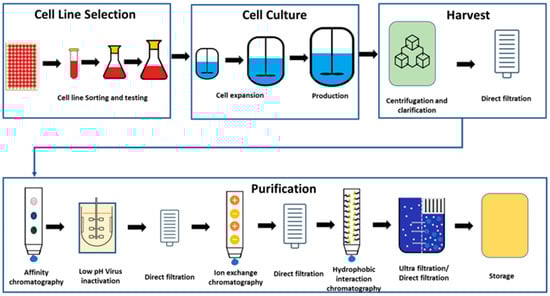
Figure 1.
General process for manufacturing of biologics drug substance.
2.3. Process Variables
Time series data collected in bioreactor production plays a critical role in monitoring and controlling the production process. These data points are typically recorded at regular intervals over time and represent various process variables that directly influence the bioreactor environment and product yield. By collecting time series data, operators can gain real-time insight into the bioreactor’s performance, allowing for proactive adjustments to maintain optimal conditions. Table 1 illustrates the list of process variables that were extracted and used for model development in the present study, with the aim of monitoring the process in real time.

Table 1.
List of process variables used in the development of the models.
Data extraction and time series data cleaning relevant to MSPM model development was extracted for a specific set of bioreactor tags (Table 1) from the online data repository. The data extraction process was carried out at two distinct frequencies (a) at every 5 min (low frequency); and (b) at every 2 min (high frequency) for activities associated with in silico data generation. The extracted data were organized in a 2D variable-wise format with N × T rows and V columns, where N was the number of real batches, T was the number of time points, and V represented the number of selected variables. The commencement and conclusion of each batch during data extraction was determined with reference to the manufacturing schedule. For data cleaning, the bioreactor vessel’s weight was considered as the primary filter. Based on recommendations from manufacturing, a specific weight limit was set to determine the running status of the bioreactor for each batch. Any rows containing data points with weight value below the set limit were discarded. Data were also cleaned to remove any abnormal excursions when appropriately justified in a risk-based approach and concurred by relevant Subject Matter Experts (SMEs)
2.4. Data Alignment and In Silico Batch Generation
In the initial phases of MSPM model development, the amount of the manufacturing batch data can be extremely limited due to the limited manufacturing experience in production scale (termed as the low-N scenario), which is particularly true for most mAbs. To effectively address this data gap for MSPM model development and build a robust process monitoring model, in silico augmented data were used in this work in conjunction with real data from manufacturing. The cleaned manufacturing data with a frequency of 2 min was aligned to have the same length before proceeding to the in silico batch generation activities. The alignment was performed with a Correlation Optimized Warping method using PLS-Toolbox Version 9.1.0 (Eigenvector Research, Inc., Manson, WA, USA) in MATLAB Version R2022a (Mathworks®, Natick, MA, USA) [21,22]. We are extracting the data at fixed frequency; hence, the number of data points per batch will be determined by the runtime of the batches. The alignment was performed in two ways: (1) aligning the batch lengths to the shortest batch, and (2) aligning the batch lengths to the longest batch. The alignment of the batches is necessary for generation of the in silico data due to the requirements of the “bGen” toolbox. Based on the process understanding and subject matter expert’s (SME’s) recommendation, any variable can be selected as a reference variable for alignment. In both cases, dissolved oxygen (DO) was used as the reference variable for the alignment process after the discussion with the upstream biologics process SMEs. The aligned data were then utilized to generate in silico batches using the MATLAB Live Script “bGen,” developed by Gasparini et al. [18] and available in the GitHub repository (https://github.com/antoniobenedetti-pmh/bGen, accessed on 14 April 2025). The resampling interval parameter in bGen was set to 50 and all other parameters kept as default. The in silico data generation method trains a Gaussian Process State-Space (GP-SS) model to generate in silico batches from high-frequency real data [18]. It employs an iterative algorithm to estimate key parameters, including the number of resampled trajectories and the memory (or lag) parameter for each variable to train the GP-SS model [18]. The validation of the in silico model is a crucial aspect of our approach. As detailed in reference [18], one challenge involves the potential loss of some information from the original experimental batches due to stratified resampling. This resampling can cause the trajectories of certain variables to exhibit less variability than in the real data. To address this, the number (J) of resampled trajectories must be carefully chosen to preserve the variability inherent in the real data. By tuning (J) and increasing the number of in silico batches, the variability required for the model can be captured. A strategy was outlined in the original paper to ensure the in silico batches mirror the variability of the experimental data. Accordingly, in this study, after each modification of J and the number of batches, the generated in silico batches are evaluated by visualizing the variables and PCA scores derived from integrated real and in silico batches. To further confirm this, the real batches should span a large portion of the score space. This approach allows identifying the optimum J value and number of batches that ensure the generated in silico batches effectively capture the dataset’s inherent variability.
2.5. Model Development and Workflow
2.5.1. Variable Classification
For the development of the models, the variables were sorted as static or dynamic (refer to Table 1). The rationale behind this segregation is to create distinct datasets for PCA and batch trajectory models. The PCA model is built to monitor static variables, while dynamic variables are monitored with the batch trajectory model.
While the differentiation between static and dynamic variables appears straightforward, the challenge of classifying these variables is obscured by their seemingly simple definitions. To eliminate the perceived subjectivity involved in classifying the variables, the following method was implemented. Initially, each variable was auto scaled. Then, for each calendar day during which a batch occurred, the mean of each process variable was calculated. For each process variable, the number of days in which the absolute value of the daily mean exceeded 1.0 was totalled. If this count surpassed 10% of the total days for which data were available, the variable was classified as dynamic; otherwise, it was classified as static. The logic behind the reasoning for this method was as follows: if the daily mean of a process variable consistently was one standard deviation below or above its batch mean for a significant portion of the batch history, it was very likely that the process variable was inherently dynamic. Furthermore, the final categorization of static and dynamic variables was validated and refined with input from Subject Matter Experts (SMEs).
2.5.2. Chemometrics Method Development
Figure 2 illustrates the workflow utilized for model development in both high-N and low-N data scenarios. In cases where there is a rich product history (high-N scenario), real batches are employed directly in model development. Conversely, in the low-N scenario, where product history is limited, in silico batches are integrated with real batches to compensate for the lack of historical data. This approach ensures the robustness and the reliability of the models. For the present study, the low-N scenario was applicable.
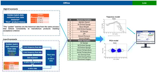
Figure 2.
Workflow for the model development and monitoring workflow for low-N and high-N data scenarios. Based on the type of the variables (dynamic and static), PCA and trajectory models were developed and deployed as separate models in Aspen Process Pulse V12.2 (Aspen Technology, Inc., Bedford, MA, USA) for real-time monitoring.
As noted above, two types of variables exist: dynamic and static. PCA and batch trajectory modelling were employed for monitoring these variables, tailored to their specific characteristics. PCA is adept at handling static variables but encounters challenges with dynamic variables because it assumes static relationships and fails to capture temporal changes. Conversely, batch trajectory modelling is essential for dynamic systems as it effectively tracks the evolution of variables over time. However, this method is not suitable for static variables, as it requires inherent variability to construct meaningful trajectories.
For both monitoring methodologies, the batches were organized in a variable-wise format merging low-frequency (5 min) real batch data and those generated in silico (50 min frequency) and imported to Unscrambler® V12.2 (Aspen Technology, Inc., Bedford, MA, USA) for further model development. The PCA model was developed using mean-centred static variables with a 95% confidence threshold and validated through cross-validation. Additional data refinement was performed by excluding outliers identified via F-residuals and Hotelling’s T2 limits to enhance model robustness and accuracy. This approach ensured that the model reliably captured relevant data patterns while maintaining stringent quality control measures.
The batch trajectory model was built in Unscrambler® V12.2 (Aspen Technology, Inc., Bedford, MA, USA) employing the assumption-free approach for trajectory modelling, as outlined by Frank Westad et al. [23]. It begins by constructing a PCA model with dynamic data to create trajectories that represent batch behaviour in the principal components space over time. A grid-search method identifies common start and end points for these trajectories. An average trajectory is established, where model distances indicate point deviations and F-residuals control limits evaluate the fit of samples to the model correlation structure. This method efficiently manages varying batch run times and process stages without the need for time warping or specific sampling frequencies. The trajectory model was constructed using mean-centred dynamic variables with a 95% confidence threshold and its validity was confirmed through cross-validation.
The developed models were deployed to the online system, Aspen Process Pulse V12.2 (Aspen Technology, Inc., Bedford, MA, USA), for real-time monitoring of the batches for the mAb case study. For the current scope of the work focused on process monitoring, when abnormalities are detected, the operators are immediately notified. They assess the situation and take the necessary corrective actions based on the specific context and nature of the abnormality observed. This approach maintains human oversight, ensuring responsiveness and adaptability to a range of potential operational conditions.
3. Results and Discussion
Model-based real-time process monitoring and process control are key areas of interest for a number of scientific fields, such as (bio)chemical processing, pharmaceutical manufacturing, and energy and gas production [17,24,25]. In this work, we have focused on developing real-time process monitoring capability based on multivariate statistical modelling approaches to monitor the performance of upstream bioreactors for the production of monoclonal antibodies (mAbs). Through the implementation of MSPM methods, we aim to track multiple variables simultaneously, offering a comprehensive view of system performance. This approach enables us to take preventative actions in response to any potential excursions, ensuring optimal system operation.
3.1. Evaluation of In Silico Batches and Comparison with Real Data
This section presents the results of using bGen to generate in silico datasets for low-N scenarios, applied to both static and dynamic variable examples. The bGen applies Gaussian process state-space models to build in silico datasets from the few historical batch datasets. In Figure 3, the red points represent the data points generated in silico, while the blue points display the real low-N data points. The two real batch data have a sampling frequency of 2 min, while in silico batches are generated with a sampling frequency of 50 min. The bounds for the in silico data were defined based on the bounds of the real data.
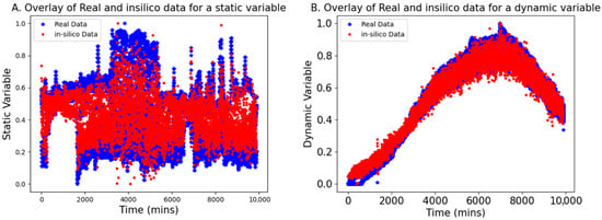
Figure 3.
Overlay of the in silico generated data (red points) with real data (blue stars) aligned according to the maximum batch length. Both (A,B) demonstrate the effectiveness of the in silico batches in covering the space bracketed by the real batches, providing satisfactory coverage for the static and dynamic data, respectively.
As seen in Figure 3, the in silico batches are contained within the bounds of the real batches and demonstrate excellent coverage of the gaps between the trajectories of real data. Furthermore, the trajectories of the in silico batches closely resemble those of the real batches. The result confirmed that even with the low-frequency data, the in silico batches completely cover the space bracketed between real data, while retaining the structure and trends of the original batches. This reconstructing of variability in data facilitates the development of robust models for further applications.
3.2. Model Development Results
3.2.1. PCA Model Result
The developed PCA model consisted of seven principal components to explain 83% variance of the ten static variables. The dataset contained two historical batches, and 20 in silico generated batches. From the scores plot in Figure 4, it is observed that there is an even distribution of the data points across the model space. The real batches (green and red solid points) are clustered on the opposite ends of the ellipse, while the in silico batches (blue solid points) occupy the space between them. This enhances the model’s coverage and its capability to capture the variability within the real batches. The green and red areas indicate process conditions that are slightly distinct from one another.
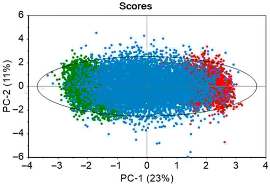
Figure 4.
Score plots of PCA model developed using the two real batches and 20 in silico batches. The ellipse illustrates the 95% confidence limit. Green and red solid points demonstrate real batches, while the in silico batches are shown with blue solid points.
3.2.2. Trajectory Model Result
Dynamic variables from 2 real batches and 20 in silico batches were utilized to develop the trajectory model for monitoring these variables. The data were mean-centred, and two principal components were considered in creating the trajectory models. The maximum grid range for dimensions 1 and 2, along with batch coverage, was set at 8, 9, and 80%, respectively. The model’s validity was confirmed through cross-validation. The model results are depicted in Figure 5. Figure 5a shows the two-dimensional trajectory score, highlighting a common trajectory for batches over relative time and indicating the start and end points of the trajectory, which correspond to the inoculation and harvesting times. In the Figure 5a, solid lines represent the average trajectory, while dashed lines indicate the two standard deviation limits. The estimated dynamic model distances and F-residuals control limits are illustrated throughout the trajectory in Figure 5b,c. Trajectory scores, model distances, and F-residual plots are monitored for any potential deviations. The application of the approach outlined in Figure 5 is further contextualized in Section 3.5 within the framework of the discussion on the illustrative case study.
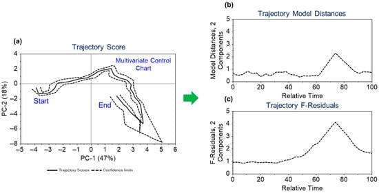
Figure 5.
Overview of (a) the scores plot for the trajectory model with mean trajectory and confidence intervals at two standard deviation limits along with its (b) trajectory model distances and (c) trajectory F-residuals control limits.
3.3. Real-Time Monitoring and Diagnostics Criteria
The developed models were deployed on the online platform ‘Aspen Process Pulse version 12.2’ developed by Aspen Technology, Inc. The univariate monitoring of the process describes the characteristics in just one dimension and only the upper and lower limit or confidence bands around the mean value. For the multivariate process monitoring, the following parameters were used for fault detection: Hotelling’s T2 and F-residual limits.
Hotelling’s T2, Equation (1), describes the behaviour of the process in the state space and identifies the correlation structure of the variables in the model using the covariance matrix used to build the model [26,27,28].
where x is observation vector with p variables, vector is the estimated mean for each variable, and t refers to the transpose operation. S is the estimated covariance of the matrix. The T2 can be calculated and plotted for each new data point [29]. The model distances in trajectory modelling are estimated similarly to the calculation of Hotelling’s T2 statistic [20].
F-residuals represent the prediction ability of the model. When the model is robust, the residuals are smaller. Also, when the projected data point from the process has variable correlation, as seen by the model from the training dataset, the residuals for the projection are small. Large residuals can indicate unusual process behaviour and a potential fault in the process [29].
For the PCA models, we used Hotelling’s T2 and F-residual limits at a 95% confidence interval as fault detection thresholds for identifying outliers. In the trajectory models, fault detection limits were set using F-residuals and model distances with a 95% confidence interval. Due to the dynamic nature of trajectory models, the limits are inherently dynamic. However, we established a static limit for outlier detection by considering only the highest value for F-residuals and Hotelling’s T2/model distances within the model. Errors or process changes were detected through signs of drift, excessive noise, or by tracking residuals/distance values over time. The models were set up to acquire and project new data every 5 min on score plots, as well as residual and Hotelling’s T2/model distances plots. Recognizing that biomanufacturing processes are comparatively slower than chemical ones, we set fault detection thresholds at 12 and 24 consecutive points outside the residual and Hotelling’s T2/model distance limits for warning and alarm alerts. These corresponded to process durations of 1 and 2 h, respectively. This approach is specifically designed to be effective, drawing on insights from monitoring real-time batches.
3.4. Model Lifecycle
Figure 6 illustrates the lifecycle of the MSPM model for biopharmaceutical manufacturing in the low-N scenario, which begins with limited historical data and progresses toward the development of the final version. Prototype MSPM models are iteratively refined by expanding the volume of real data and generating new in silico data through retraining the GPSS model. This iterative process incorporates additional data from new batches, progressively enhancing the model’s data. Once a prototype demonstrates robust performance and meets predefined sensitivity criteria, it is designated as the final version. Additionally, as sufficient batches of real data become available, subsequent models can be developed solely using real data, thereby eliminating the reliance on in silico data generated by the GPSS model. Throughout the process, regular engagement with manufacturing subject matter experts is critical to identify false positive and false negative detections, with the aim of enhancing the model’s performance and validating its accuracy as part of the continuous improvement framework.
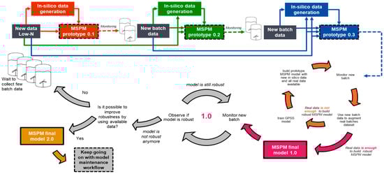
Figure 6.
Lifecycle of the MSPM model: from limited data to final version development.
3.5. Case Study of the Application of the MSPM Model—Detection of the Drifting pH and Failure of a pH Probe
This case study covers the detection of the failure of a pH probe through the batch trajectory model. The relative functioning of the primary and secondary pH probes in the bioreactors is monitored using a variable called pH probe difference. This value for the variable is calculated by subtracting the values measured by primary and secondary pH probes fitted within the bioreactor vessel. In an ideal condition, the value for this variable should be zero, but for normal functioning, the tolerance for the accepted value for the pH probe difference variable is up to 0.07.
In the given instance, the secondary pH probe had failed and the MSPM models were able to pick up the trend in the variable, with an excursion reported on the trajectory scores (as well as on the F-residuals for the model). Figure 7a,b illustrates the developed score plot and the score plot with the projected faulty batch, respectively. The projected batch points (blue solid points in Figure 7b) are shown to deviate from the normal trajectory limits.
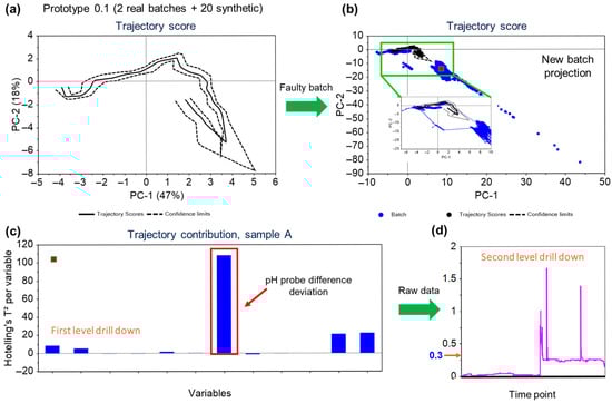
Figure 7.
Overview of the workflow for fault detection—(a) The trajectory scores plot for model for the process built using the real data from historical runs and in silico process generated to capture missing data correlations. The solid line represents the mean trajectory, and the dashed lines are the confidence limits. (b) Trajectory scores plot for the batch (blue) projected over the model. The projected batch is significantly outside the model confidence bands and hence is classified as an excursion. (c) First level drilldown of the variables contributing to the excursion, indicating pH probe difference has the highest contribution to the deviation. (d) Second level drilldown—The acceptable process limit for the pH probe difference was 0.07 but the data shows the values crossed 0.3 and stayed beyond the limit.
The variables contributing to the projection of the points can be confirmed from the correlations plot Figure 7c. As seen in Figure 7d, value for the pH probe difference variable had jumped to more than 1.5. An immediate action was taken to replace the probe, and the trend returned to the normal functioning limits. The pH of the bioreactor was not significantly affected as it is controlled using the primary probe with the secondary probe as a back-up. In this case, although the process itself was not impacted due to the secondary pH probe failure, the equipment defect was promptly addressed leveraging the MSPM model-based observations. This scenario exemplifies the crucial role of process monitoring during manufacturing operations to ensure the consistency and the robustness of the process. It not only enables swift responses to deviations in process parameters but also facilitates the early detection and resolution of equipment failures.
4. Conclusions
In this article, we demonstrate the application of the Multivariate Statistical Process Monitoring (MSPM) models in the detection and correction of atypicality within biopharmaceutical manufacturing processes during production, compared to the historical multivariate dataspace. By integrating both real and in silico data in low-N scenarios utilizing the GPSS model, we developed robust models that can monitor both static and dynamic variables effectively using the online platform. This is particularly significant as low-N scenarios are common in biopharmaceutical processes, especially during early CMC phases of development, and our successful implementation of the GPSS model emphasizes the applicability and efficacy of this approach. To effectively monitor all process parameters, we developed two models: the PCA model, which includes static variables that traditionally serve as process set points; and the trajectory model, which captures the relationships between dynamic variables that evolve throughout the batch process. The detection parameters Hotelling T2/model distances and F-residuals were used to identify the excursions. When multiple consecutive excursions were flagged going beyond the confidence limits, an alarm was triggered indicating process deviation to alert our production engineers. This enabled them to take timely corrective action and investigate the root cause, preventing potential failures and ensuring that the process remained in optimal production condition. Utilizing multivariate statistical process modelling to identify process atypicality, as opposed to relying solely on univariate trends, offers significant industrial advantages. This approach can significantly reduce costs by preventing batch failures in a preventative manner, as well as confirming equipment health on an ongoing basis, when appropriately implemented within the manufacturing setting. Furthermore, it enhances the efficiency and the productivity of the biopharmaceutical manufacturing processes. Thus, deploying this method is highly recommended during the routine production of biopharmaceuticals.
Author Contributions
Conceptualization, S.M., S.B. and G.B.; formal analysis, S.M., S.B., G.M. and E.A.; resources, G.B. and S.C.; data curation, S.M., S.B., G.M., E.A., N.B. and T.V.; writing—original draft preparation, S.M., S.B., G.M. and E.A.; writing—review and editing, S.M., S.B., G.M. and S.C. All authors have read and agreed to the published version of the manuscript.
Funding
This research received no external funding.
Data Availability Statement
The datasets presented in this article are not readily available because they contain proprietary GSK data. Requests to access the datasets should be directed to sushrut.x.marathe@gsk.com.
Acknowledgments
Helpful discussions with Connor Gallagher, Brian Rhodes, Luke Bellamy from GSK are gratefully acknowledged.
Conflicts of Interest
The authors declare no conflict of interest. All authors were employed by GSK at the time of this study. All authors declare that the research was conducted in the absence of any commercial or financial relationships that could be construed as a potential conflict of interest.
Abbreviations
The following abbreviations are used in this manuscript:
| mAbs | Monoclonal antibodies |
| MSPM | Multivariate statistical process monitoring |
| PCA | Principal component analysis |
| ADCs | Antibody drug conjugates |
| C>s | Cellular and gene therapies |
| PLS | Partial least square |
| CLT | Central-limit theorem |
| O2 | Oxygen |
| CO2 | Carbon dioxide |
| DO | Dissolved oxygen |
| N2 | Nitrogen |
| Add PMP ttlzr | Additional Pump Totalizer |
| pH probe diff | pH probe difference |
| MFC | Mass Flow Controller |
References
- Flickinger, M.C. Upstream Industrial Biotechnology, 2 Volume Set; John Wiley & Sons: Hoboken, NJ, USA, 2013. [Google Scholar]
- Walsh, G.; Walsh, E. Biopharmaceutical benchmarks 2022. Nat. Biotechnol. 2022, 40, 1722–1760. [Google Scholar] [CrossRef]
- Velugula-Yellela, S.R.; Williams, A.; Trunfio, N.; Hsu, C.J.; Chavez, B.; Yoon, S.; Agarabi, C. Impact of media and antifoam selection on monoclonal antibody production and quality using a high throughput micro-bioreactor system. Biotechnol. Prog. 2018, 34, 262–270. [Google Scholar] [CrossRef]
- Reuveny, S.; Velez, D.; Macmillan, J.D.; Miller, L. Factors affecting cell growth and monoclonal antibody production in stirred reactors. J. Immunol. Methods 1986, 86, 53–59. [Google Scholar] [CrossRef]
- Tang, M.; Yang, C.; Gui, W. Fault detection based on cost-sensitive support vector machine for alumina evaporation process. Control Eng. China 2011, 18, 645–649. [Google Scholar]
- Ge, Z.; Song, Z. Multivariate Statistical Process Control: Process Monitoring Methods and Applications; Springer Science & Business Media: Berlin/Heidelberg, Germany, 2012. [Google Scholar]
- Peng, K.; Zhang, K.; Li, G.; Zhou, D. Contribution rate plot for nonlinear quality-related fault diagnosis with application to the hot strip mill process. Control Eng. Pract. 2013, 21, 360–369. [Google Scholar] [CrossRef]
- Chen, Z.; Zhang, K.; Hao, H.; Ding, S.X.; Krueger, M.; He, Z. A canonical variate analysis based process monitoring scheme and benchmark study. IFAC Proc. Vol. 2014, 47, 10634–10639. [Google Scholar] [CrossRef]
- Lou, Z.; Wang, Y.; Si, Y.; Lu, S. A novel multivariate statistical process monitoring algorithm: Orthonormal subspace analysis. Automatica 2022, 138, 110148. [Google Scholar] [CrossRef]
- Qin, S.J. Survey on data-driven industrial process monitoring and diagnosis. Annu. Rev. Control 2012, 36, 220–234. [Google Scholar] [CrossRef]
- Wold, S.; Esbensen, K.; Geladi, P. Principal component analysis. Chemom. Intell. Lab. Syst. 1987, 2, 37–52. [Google Scholar] [CrossRef]
- Liu, L.; Liu, J.; Wang, H.; Tan, S.; Yu, M.; Xu, P. A multivariate monitoring method based on kernel principal component analysis and dual control chart. J. Process Control 2023, 127, 102994. [Google Scholar] [CrossRef]
- Macgregor, J.F.; Kourti, T. Statistical process control of multivariate processes. Control Eng. Pract. 1995, 3, 403–414. [Google Scholar] [CrossRef]
- Zomer, S.; Zhang, J.; Talwar, S.; Chattoraj, S.; Hewitt, C. Multivariate monitoring for the industrialisation of a continuous wet granulation tableting process. Int. J. Pharm. 2018, 547, 506–519. [Google Scholar] [CrossRef]
- Rato, T.J.; Delgado, P.; Martins, C.; Reis, M.S. First principles statistical process monitoring of high-dimensional industrial microelectronics assembly processes. Processes 2020, 8, 1520. [Google Scholar] [CrossRef]
- Chiang, L.H.; Braun, B.; Wang, Z.; Castillo, I. Towards artificial intelligence at scale in the chemical industry. AIChE J. 2022, 68, e17644. [Google Scholar] [CrossRef]
- Nikolakopoulou, A.; Yang, O.; Bano, G. Real-Time Statistical Process Monitoring; CRC Press: Boca Raton, FL, USA, 2024; pp. 303–323. [Google Scholar]
- Gasparini, L.; Benedetti, A.; Marchese, G.; Gallagher, C.; Facco, P.; Barolo, M. On the use of machine learning to generate in-silico data for batch process monitoring under small-data scenarios. Comput. Chem. Eng. 2024, 180, 108469. [Google Scholar] [CrossRef]
- Shukla, A.A.; Thömmes, J. Recent advances in large-scale production of monoclonal antibodies and related proteins. Trends Biotechnol. 2010, 28, 253–261. [Google Scholar] [CrossRef] [PubMed]
- Birch, J.R.; Racher, A.J. Antibody production. Adv. Drug Deliv. Rev. 2006, 58, 671–685. [Google Scholar] [CrossRef]
- Christin, C.; Smilde, A.K.; Hoefsloot, H.C.; Suits, F.; Bischoff, R.; Horvatovich, P.L. Optimized time alignment algorithm for LC-MS data: Correlation optimized warping using component detection algorithm-selected mass chromatograms. Anal. Chem. 2008, 80, 7012–7021. [Google Scholar] [CrossRef]
- Tomasi, G.; Van Den Berg, F.; Andersson, C. Correlation optimized warping and dynamic time warping as preprocessing methods for chromatographic data. J. Chemom. A J. Chemom. Soc. 2004, 18, 231–241. [Google Scholar] [CrossRef]
- Westad, F.; Gidskehaug, L.; Swarbrick, B.; Flåten, G.R. Assumption free modeling and monitoring of batch processes. Chemom. Intell. Lab. Syst. 2015, 149, 66–72. [Google Scholar] [CrossRef]
- Kumar, P.; Rawlings, J.B.; Wenzel, M.J.; Risbeck, M.J. Grey-box model and neural network disturbance predictor identification for economic MPC in building energy systems. Energy Build. 2023, 286, 112936. [Google Scholar] [CrossRef]
- Schaeffer, J.; Lenz, E.; Gulla, D.; Bazant, M.Z.; Braatz, R.D.; Findeisen, R. Gaussian process-based online health monitoring and fault analysis of lithium-ion battery systems from field data. Cell Rep. Phys. Sci. 2024, 5, 102258. [Google Scholar] [CrossRef]
- Sivasamy, A.A.; Sundan, B. A Dynamic Intrusion Detection System Based on Multivariate Hotelling’s T2 Statistics Approach for Network Environments. Sci. World J. 2015, 2015, 850153. [Google Scholar] [CrossRef] [PubMed]
- Ye, N.; Emran, S.M.; Chen, Q.; Vilbert, S. Multivariate statistical analysis of audit trails for host-based intrusion detection. IEEE Trans. Comput. 2002, 51, 810–820. [Google Scholar] [CrossRef]
- Chou, Y.M.; Mason, R.L.; Young, J.C. Power comparisons for a Hotelling’s T2 statistic. Commun. Stat. Simul. Comput. 1999, 28, 1031–1050. [Google Scholar] [CrossRef]
- Tatara, E.; Çinar, A. An intelligent system for multivariate statistical process monitoring and diagnosis. ISA Trans. 2002, 41, 255–270. [Google Scholar] [CrossRef]


Disclaimer/Publisher’s Note: The statements, opinions and data contained in all publications are solely those of the individual author(s) and contributor(s) and not of MDPI and/or the editor(s). MDPI and/or the editor(s) disclaim responsibility for any injury to people or property resulting from any ideas, methods, instructions or products referred to in the content. |
© 2025 by the authors. Licensee MDPI, Basel, Switzerland. This article is an open access article distributed under the terms and conditions of the Creative Commons Attribution (CC BY) license (https://creativecommons.org/licenses/by/4.0/).