Article

Modeling Power Consumption: A Novel Correlation for Stirred Media Mills with Variable Bead Filling Ratios

by
Simay Ozsoysal
1,*,
Hamidreza Heidari
1,
Gulenay Guner
2,
Donald J. Clancy
2 and
Ecevit Bilgili
1,†
1
Otto H. York Department of Chemical and Materials Engineering, New Jersey Institute of Technology, Newark, NJ 07102, USA
2
Drug Product Development, Medicine Development & Supply, GSK R&D, Collegeville, PA 19426, USA
*
Author to whom correspondence should be addressed.
Ecevit Bilgili passed away before the submission of this paper.
J. Pharm. BioTech Ind. 2025, 2(3), 14; https://doi.org/10.3390/jpbi2030014
Submission received: 31 July 2025 / Revised: 28 August 2025 / Accepted: 30 August 2025 / Published: 8 September 2025

Abstract

Evaluating power consumption in stirred media mills over a wide range of process parameters is crucial for analyzing breakage kinetics and milling efficiency. Despite considerable research efforts, existing models predominantly rely on power-law approaches and fail to provide a holistic understanding of the relationship between process parameters and power consumption. The aim of this study is to introduce a new mathematical model that accurately captures this relationship, across all bead filling ratios (φ), using dimensionless numbers including power number (Ne) and Reynolds number (Re). First, we considered experimental data from literature and discriminated various models to correlate either Ne or Re separately for each φ (Class 1 models) or Ne to Reφ simultaneously (Class 2 models). The best performing model (Model 2.6 with SSR = 36.71, RMSE = 0.591, R2 = 0.99) was subsequently applied to a new set of experimental data, confirming that this model is highly robust and reliable across various conditions. To the best of our knowledge, in stirred media mill research, this work is the first to show that a simple four-parameter nonlinear model provides a robust fit for Ne data across varying rotor Re (200 to 1 × 10⁶) and bead filling ratios (0.35–0.90).

Graphical Abstract

1. Introduction

Stirred media mills are widely used across several industries, particularly in mineral processing [1,2,3] and pharmaceuticals [4,5,6]. They are characterized by their capability of producing sub-micron-sized particles, making them highly effective for ultrafine grinding applications [7]. Reducing particle size to sub-micron range is a key factor in achieving greater uniformity, solubility, and strength, thus ensuring better product quality [8]. To that end, stirred media mills have attracted considerable attention from industry and researchers in recent years due to their ability to achieve ultrafine grinding through strong impact forces [9]. In addition to enabling control over particle size distribution, they also aid in minimizing the margin of error during the production of critical materials [10].
Despite their advantages, stirred media mills are also known for high energy demands and significant operational costs [11]. High energy input can lead to significant heat generation, temperature rise, and potential amorphization [12,13,14]. Maintaining proper temperature is essential since it can influence both the physical and chemical stability of a drug suspension during the milling process [15]. These drawbacks constrain implementation of stirred media mills in certain industries [16]. Optimizing the process parameters, such a bead filling ratio (φ), mill speed (ω), and bead size (Db), can notably minimize energy consumption [17] and reduce operational costs while achieving the desired product particle size [13,18]. To achieve this, the correlation between process parameters and power consumption should be closely examined, as it is highly important for assessing breakage kinetics and milling efficiency [19,20].
To date, several publications have concentrated on understanding and predicting mill power consumption [19,21,22,23,24,25,26,27,28]. Some researchers have formulated predictive models using dimensionless numbers, such as power number (Ne) and Reynolds number (Re) to predict power consumption, while others have relied on dimensional process parameters , ω, etc.). A common feature observed within these studies is the use of power-law equations, in which multiple process parameters are expressed as specific exponents, and the equation is formed by multiplying these parameters together [29]. However, the use of power-law equations to predict power consumption has multiple drawbacks, as such models oversimplify the relationship between process parameters and power consumption. Additionally, they do not provide a comprehensive understanding of the underlying physics that govern energy transfer, heat generation, or fluid–particle interactions. Taking everything into account, it is essential to further investigate this relationship and develop a model that does not rely on power-law equations.
Several mathematical models have been derived describing the relationship between Ne and Re in a stirred media mill, operating with and without milling media (grinding beads) [22]. These models provide a fundamental basis for understanding the link between process parameters and the power consumption; however, they have notable limitations. One limitation arises from deriving equations based on the segmentation of fluid flow into laminar, transition, and turbulent regions, where the relationship between Ne and Re in each region is defined by a separate mathematical equation. Researchers have to switch between models according to flow conditions, emphasizing the need for a unified, continuous model to capture the entire flow behavior in a continuous and accurate way. Another limitation is the dependence of the NeRe relationship on the specific bead filling ratio, φ. To the best of our knowledge, no comprehensive mathematical model has been developed so far that could fully capture the relationship of Ne and Re across different bead filling ratios.
The primary objective of this paper is to demonstrate that the correlation between process parameters and power consumption can be effectively captured using a novel, well-formulated model (applicable to any flow regime and bead filling ratio) based on dimensionless numbers, Ne and Re. To this end, we collected experimental data from a literature source, implemented several mathematical fitting models, performed statistical analysis to determine the most reliable model, and validated the best-performing model using a different set of experimental data. Our findings are that the mathematical equation developed in our study (that does not rely on power-law equations) effectively captures the NeRe relationship through all three flow regimes and accurately accounts for the bead filling ratio effect. Our model is designed to be simple and compact, enabling practical application for researchers to apply in real-world scenarios while minimizing computational cost.

2. Materials and Methods

2.1. Data Collection (from Experimental Work)

2.1.1. Data for Model Development

The foundation of our study was built on experimental data acquired from a published article by Kwade and Schwedes [22], who explored the use of three bead filling ratios (φ = 0.35, φ = 0.65, and φ = 0.90) in a stirred media mill operating with 1 mm glass beads. Data points (illustrating the NeRe relationship) were extracted from Figure 60 in Ref. [22] using PlotDigitizer (3.3.9 PRO Version).

2.1.2. Data for Model Validation

A new set of experimental data was used to further test and compare the performance of the two leading mathematical models under new conditions. This dataset, comprising of a total of 12 data points, was derived from an experimental study by Heidari et al. [30] utilizing 400 µm Zirmil Y-grade yttrium-stabilized zirconia (YSZ) beads in a Netzsch Microcer wet stirred media mill (large batch), with variations in stirrer speed (2000–4000 rpm) and bead loading (0.4–0.6).

2.2. Theoretical

Analyzing dimensionless numbers, particularly power number and Reynolds number, is highly useful for developing power consumption models, given their extensive use in stirrer technologies [15,31,32]. Given the complexity of the stirring motion, dimensional analysis serves as a useful tool to identify the correlation between power consumption and the governing variables [33]. This correlation also highlights its nonlinear nature through the significant shifts in power number between flow regions. Power number and Reynolds number can be expressed by the following equations, respectively [22,34,35,36]:
N e = P D r 5 ω 60 3 ρ s
R e = ω 60 D r 2 ρ s μ s
where P (Watt, kg m 2 s 3 ) stands for the total power consumption within the stirred media mill, Dr (m) is the diameter of the mill rotor, and ω (RPM, revolutions per minute) is the stirring speed. The factor of 60 in both equations arises from the conversion of mill speed from revolutions per minute to revolutions per seconds. The density and dynamic viscosity of the suspension are represented by ρ s ( k g m 3 ) and μ s ( k g m · s ), respectively. It is assumed that the beads are part of the equipment design; they are not considered as part of the suspension. In other words, only the equivalent liquid (liquid and material ground) is considered in the Re definition, but not the beads.

2.2.1. Mathematical Models

A total of 13 mathematical models, comprising both novel formulations and models derived from existing literature were tested on the dataset to identify the one that achieved the best fit. These mathematical models were primarily classified into two groups for in-depth analysis (see Figure 1). The first group, known as Class 1, included six fitting models where Ne was formulated solely based on Re; whereas the latter group, referred to as Class 2, consisted of seven fitting models in which Ne was influenced by both Re and φ. The models of Class 1 serve as an initial step in understanding the NeRe relationship but are limited by their inability to account for bead filling ratio, φ. Since φ is not explicitly included in equations as a variable, these models are not adaptable across different bead filling ratios; a new equation must be developed for each specific bead condition.
Table 1 and Table 2 each present a whole set of equations formulated for Class 1 and Class 2 models, respectively. Here, the superscript (i) notation is used in Table 1 to distinguish different bead filling ratios. This suggests that any variation in the bead filling ratio results in changes to the coefficients (K, Y, a1, a2, etc.). In contrast to Class 1 models, Class 2 models incorporate bead filling ratio as a variable, allowing them to be used across different bead filling ratio values without requiring individual equation modifications. Due to this general applicability, the superscript (i) notation is excluded from Table 2.

2.2.2. Statistical Analysis

All model fittings were performed using R [37] within the RStudio [38] (Version 2023.03.0+386) integrated development environment. The parameter estimation process utilized the Nelder–Mead algorithm (implemented in the nloptr [39] package in R), which iteratively optimized the parameters by minimizing the sum of squared residuals (SSR).

3. Results and Discussion

3.1. Class 1 Models for Ne–Re Correlations

The foundation for the equations of Model 1.0a and Model 1.0b is based on a single-fitting approach within a particular region (either the lower transition or the whole transition region). In essence, Model 1.0b represents an advancement over Model 1.0a, as the fit improves when the transition region is involved entirely. In both of these models, the whole turbulent region is excluded from the fitting process, because at high Reynolds numbers, Ne exhibits a nearly horizontal trend in logarithmic scale. Although Ne exhibits a slight decrease in practice, treating it as constant simplifies the overall model. A comparable fitting approach in literature can be observed in Figure 61 from the excellent publication by Kwade and Schwedes [22], which illustrates the power draw in stirred media mills with various stirrer discs. Models 1.1–1.3 follow the same region-based segmentation approach as Model 1.0a and Model 1.0b; however, rather than a single fitting, a unique equation is applied to each region, leading to a total of four equations per bead filling ratio to generate one curve. The primary differences between Models 1.1–1.3 are as follows: in Model 1.1, K values are region-dependent (K1K2K3K4). In Model 1.2, they are treated as equal across all regions (K1 = K2 = K3 = K4 = K). Model 1.3 assumes K values to be the same except in the upper turbulent region (K1 = K2 = K3 = KK4), where a different K is used due to the last region’s horizontal behavior, contrasting with the downward trend in the preceding regions. The development of these models was inspired by the equations documented in Table 2 (p. 109) of the publication of Kwade [35]. Unlike the other models in Class 1, Model 1.4 is uniquely structured; it does not follow a power-law structure and is not developed through flow-region-based classification. Our starting point for Model 1.4 was to investigate the relationship between the drag coefficient, Cd and Re. (Readers seeking further details on various formulations on CdRe correlations, may consult an extensive and informative review by Goossens [40].) We particularly inspected an empirical equation for drag coefficient of spherical particles, derived by Khan & Richardson [41], and modified it by introducing unknown parameters (a1, a2, a3, and a4) in place of constants. This allowed us to create a more adaptable and generalizable model, which proved to be effective for predicting NeRe correlations.
Graphical representations of Class 1 models across different bead filling ratios are depicted in Figure 2. Graphs clearly indicate that Model 1.0a (Figure 2a) and Model 1.0b (Figure 2b) demonstrated poor fitting performance, which was anticipated due to their oversimplification and single-fitting approach and inability to account for nonlinear effects. The adoption of a multi-region fitting strategy (Figure 2c–e), rather than relying on a single fitting (Figure 2a,b), contributed to the overall enhancement in fitting performance. However, due to the models’ reliance on the power-law framework, the fitting curves display a straight-line on a logarithmic scale, which in turn leads to discontinuities. Moreover, models with various adjustable parameters tend to demand large datasets to support accurate estimation, thereby limiting their practicality in real-world scenarios where data availability may be constrained. Yet, these models are useful to explore the relationship between parameter quantity and model performance. As the number of parameters increase, fitting improves; however, this also results in higher risk of overfitting, necessitating a careful balance in model design. Figure 2f outperforms other Class 1 models in terms of fitting performance. Since Model 1.4 does not rely on a power-law framework or region-based segmentation, it produces a smooth, continuous curve while maintaining a high level of accuracy.
Although graphical representation provides valuable information on fitting performance, carrying out a statistical analysis of parameters is equally important. Given the extensive number of parameters in Class 1 models, statistical analysis results are provided in the Supplementary Materials. Tables S3 and S6 reveal that Models 1.1 and 1.4 contain several parameters that are statistically insignificant. However, these same models seem to produce the best graphical fits (see Figure 2c,f), illustrating a key issue: satisfactory visual fits do not necessarily imply statistical robustness or accurate trend modeling. Notably, Models 1.0a and 1.0b, despite displaying the least satisfactory visual fits (see Figure 2a,b), have all parameters statistically significant (Tables S1 and S2), further emphasizing the limitations of relying solely on visual interpretation. Readers may refer to the Supplementary Materials for a more comprehensive overview of estimates, T-values, p-values, standard errors (SE), and statistical significance of parameters.

3.2. Class 2 Models for Ne–Re–φ Correlations

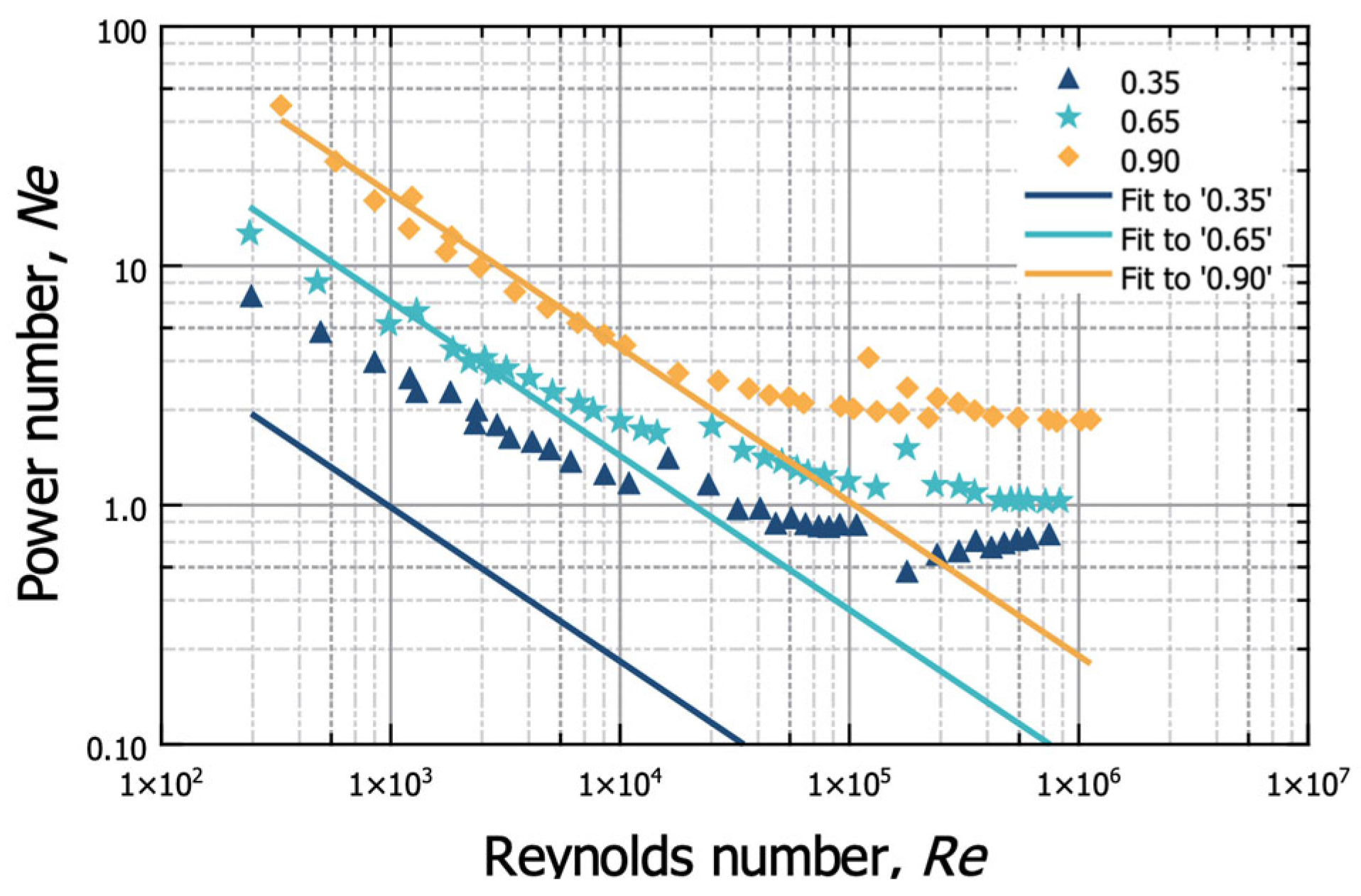
Model 2.0 is the simplest power-law model that is applied to the whole Re domain from ~200 to 1 × 10⁶. It relies on a single equation, indicating that as parameter complexity grows, achieving an appropriate fit within a power-law structure becomes increasingly difficult. A related effort has been described in literature, but with a more advanced version. Guner et al. [15] proposed a power-law correlation as the fitting model; which differs from ours by including bead size effects in addition to bead loading. They reported that the model achieved a reasonably good fit (R2 = 0.86), with some deviations. In contrast, Model 2.0, developed without bead size considerations, was unable to produce a good fit. As illustrated in Figure 3, Model 2.0 exhibits significant deviation from the observed data. Nevertheless, this model was viewed as a preliminary effort toward incorporating the bead filling ratio effects, which were not accounted for in Class 1 models.
Models 2.1–2.6 are depicted in Figure 4. The region-based segmentation and equation structures in Models 2.1–2.3 mirror those in Models 1.1–1.3, with the notable difference that φ is explicitly included as an additional parameter. The fitting performance of Models 2.1–2.3 are displayed in Figure 4a–c. A direct comparison between Figure 2c–e and Figure 4a–c suggests that the addition of an extra parameter causes a noticeable deterioration in fitting performance for each case. Given that power-law equations fail to provide a satisfactory fit, alternative mathematical approaches involving transformations of variables were considered as well. Accordingly, we formulated quadratic (Model 2.4) and cubic (Model 2.5) multiple linear regression equations based on logarithmically transformed variables. The use of log-transformed variables resulted in better fitting performance (see Figure 4d,e). Despite their high proficiency in representing the NeRe relationship, the inclusion of several variables (six and ten parameters, respectively) in these models suggests the need for developing a more compact and efficient mathematical formulation. In line with this, we formulated a simple, compact equation with only four parameters, that offers significant benefits in terms of computational efficiency and predictive accuracy (see Model 2.6 in Table 2). Since data points exhibit a pattern that aligns with equations used in friction factor correlations in pipe flows, we opted for the equation proposed by Fang et al. [42,43] as the starting point, and made appropriate modifications to the equation to align it with our specific needs. These modifications include replacing constants with unknown parameters denoted as a1, a2, a3, etc.; substituting relative roughness (ε/D) with φ; and adopting Newton number as an alternative to friction factor, f. Model 2.6 demonstrated exceptional fitting performance (see Figure 4f and Table 3), proving to be highly reliable and robust, as anticipated, and was identified as the best-performing model.
It is worth mentioning that the models shown in Figure 4d–f closely resembled one another, making visual comparison difficult. Therefore, we investigated the statistical significance of each parameter within these models (detailed in the Supplementary Materials); the analysis revealed that Model 2.5 contained an insignificant parameter, whereas all parameters of Models 2.4 and 2.6 remained statistically significant. Based on these findings, we selected these two best-performing models (Model 2.4 and Model 2.6) and evaluated their performance on a completely new dataset from a prior study [30]. The predictive performance and evaluation of these models are discussed in the Model Validation (Section 3.4).

3.3. Overview of Class 1 and Class 2 Models

A variety of conclusions can be drawn from Class 1 models. First, Class 1 models highlight the shortcomings of power-law equations, which have long been the standard approach for modeling power consumption in stirred media mills. Second, they reveal that flow-region segmentation might not consistently improve model outcomes. Third, they confirm the feasibility of developing an equation that effectively accounts for nonlinear behavior. Since Class 1 models do not explicitly account for the impact of φ on Ne, they lack generality and estimation capability for different bead filling ratios. Nevertheless, they serve as a baseline for the development of more advanced models (Class 2 models) that explicitly account for bead filling ratio effects.
An overall analysis of the fitting representation, statistics, and the standard errors of the parameters in Class 2 models, allows us to draw the following conclusions:
The drastic deviation of Model 2.0 (the standard power-law function) from the experimental data clearly demonstrates that Ne = f(Re, φ) cannot be factorized in the form of a power-law function for the whole Re domain. The fitting quality was significantly improved upon piece-wise application of the power-law model over the Re domain (Models 2.1–2.3); however, discontinuities are present along with significant deviations for the low beads loading (φ = 0.35). Considering that Models 2.1, 2.2, and 2.3 have 11, 8, and 9 parameters, respectively, the relatively low fitting quality (see fitting discrepancies in Figure 4a–c) compared to other Class 2 models is not acceptable. Instead of fitting data in four regions of the Re domain, one can simply fit the lower transition regions (120 < Re < 8000) and the highly turbulent region (Re > 105) only, which will significantly reduce the number of parameters and the number of discontinuities.
The polynomial models of the log-transformed variables (Ne, Re, and φ) did not exhibit any discontinuity; they fitted data for all three bead loadings reasonably well. As expected, the cubic polynomial fitted the data better than the quadratic polynomial. The parameters associated with the interaction and higher-order terms in both polynomial models were statistically significant (except a6 in the cubic model, see Table S12 in the Supplementary Materials). This fact points to the non-factorizability of f ( R e ,   φ ) in the power-law form as mentioned earlier. It can be easily shown that these polynomial models are equivalent to the power-law model in the absence of the aforementioned terms of the polynomial. Most importantly, the quadratic polynomial model and the cubic polynomial model have 6 and 10 parameters. Hence, a simpler model with fewer parameters and better fitting capability is still warranted.
Model 2.6, the true nonlinear model, which cannot be linearized by any transformation, outperformed all other models despite having only four parameters. Approximate standard error computations proved its parameters were statistically significant. The consistency and adaptability of the model was examined using an alternative dataset, as detailed in the subsequent section.

3.4. Model Validation

Model 2.6, when tested alongside the second-best performing model (Model 2.4) using a completely new dataset (see [30]), displayed excellent fitting performance (see Table 4). The improved performance of Model 2.6 can be attributed to the statistical significance of all its parameters (see Table S15 in the Supplementary Materials), contributing to the model’s robustness. On the other hand, Model 2.4 contained three statistically insignificant parameters (a2, a4, and a5; see Table S14 in SM), all associated with bead filling ratio. Removing these parameters to improve model validity would result in a model that fails to incorporate bead filling ratio effects.
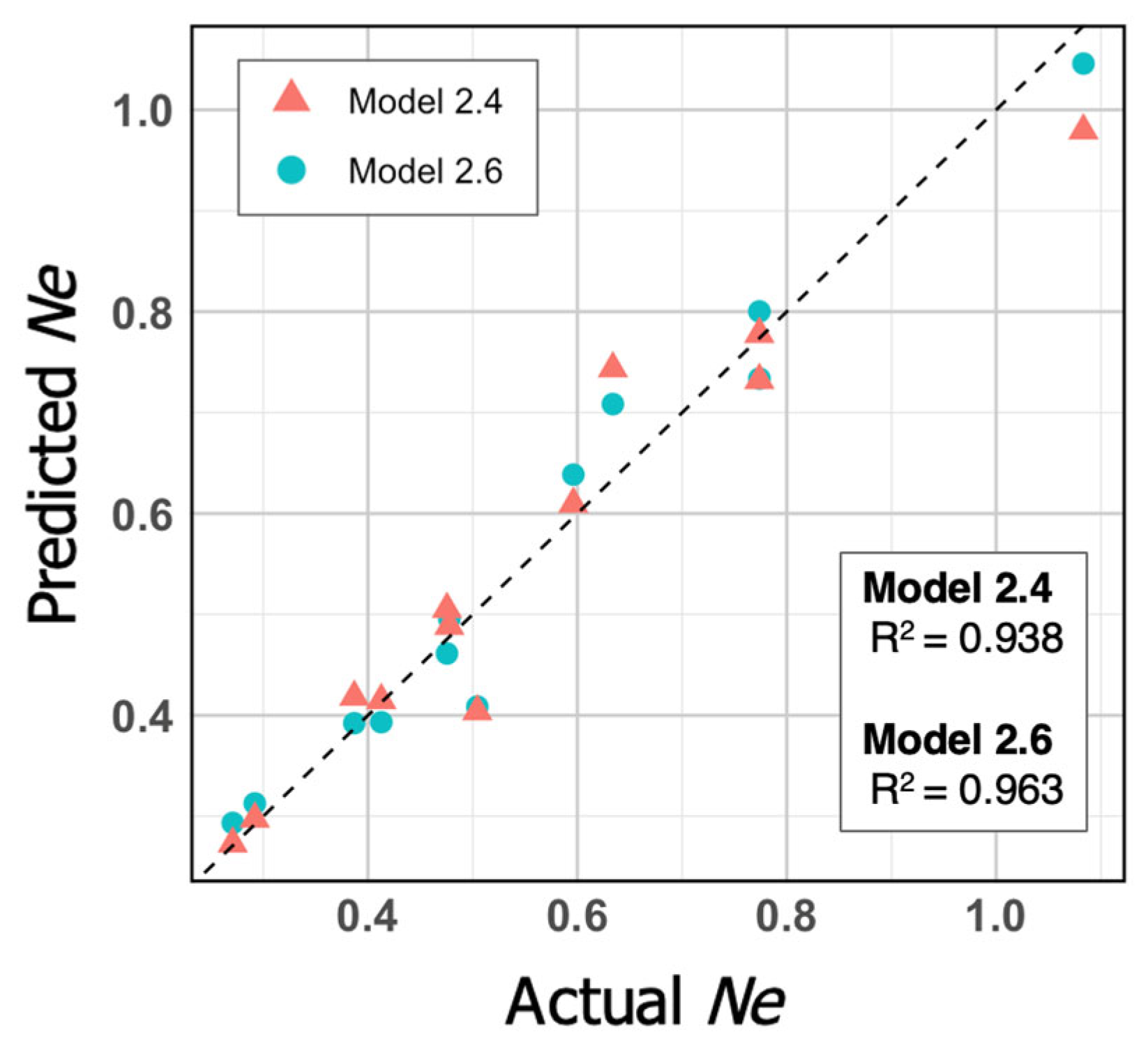
Figure 5 illustrates the equivalency plot (predicted Ne vs. experimental Ne) for both Model 2.4 and Model 2.6. The higher R2 value of Model 2.6 indicates its enhanced fitting performance. This can be attributed to several factors, one of which is that each parameter in the model contributes meaningfully to its fitting accuracy, ensuring efficient use of parameters. Additionally, the reduced set of parameters helps minimize computational cost and processing time. Furthermore, its applicability across all flow conditions removes the need for region-based segmentation, enhancing its overall robustness and versatility. Taking everything into consideration, Model 2.6 ensures smooth continuity and accurate NeRe predictions.
It should be emphasized that while Model 2.6 was initially developed for 1 mm glass beads, its ability to perform with 0.4 mm YSZ beads is a promising result. The model’s applicability to a different bead size and type may be explained by the stronger impact of bead filling ratio on power consumption. Multiple experimental studies in the literature further confirm this observation. For instance, Guner et al. [13] revealed that although bead size contributed to grinding performance, their effects were comparatively minor relative to bead filling ratio. Similarly, Altun et al. [44] demonstrated that filling ratio mainly affected specific energy consumption in stirred milling systems. Since bead filling ratio is consistently identified as one of the major determinants of energy consumption, the performance of Model 2.6 remains reliable across bead sizes.
Although current understanding of bead type (and bead density) effects on power consumption is limited, it has been reported that bead type contributes to variations in power consumption [45]. This area, however, still requires further investigation. In this study, the use of two distinct bead types in datasets (glass and YSZ beads), naturally suggests some degree of variability in power consumption. Nevertheless, these differences are not expected to be dominant, as the bead filling ratio plays the primary role in governing collision dynamics and power consumption. Overall, although Model 2.6 does not guarantee consistent fitting success in all scenarios, validation results highlight its potential to handle systems with different bead sizes and types. Future experimental work with varied bead sizes and types could provide more insights into the model’s broader applicability, especially in cases where density differences are extreme. With an expanded dataset, machine learning methods such as Random Forest, can be applied to examine relationships under more complex conditions.

4. Conclusions

For the first time in the stirred media mill literature, a simple four-parameter nonlinear model was shown to fit Ne data over a wide range of rotor Re (200 to 1 × 10⁶) and bead filling ratios, φ (0.35–0.90). Unlike the commonly held notion that N e =   f ( R e ,   φ ) can be expressed in factorized form (power-law model), both the experimental data and the model fits refute this notion. Only a truly nonlinear model could fit the data well with statistically significant parameters. This compact model (Model 2.6) enables process engineers to accurately correlate mill energy data with different bead filling ratios and stirrer speeds, as the proposed model consists of just four parameters. The successful implementation of this model under a new set of experimental conditions provides significant evidence that the model is likely broadly applicable to a variety of mill conditions and configurations.

Supplementary Materials

The following supporting information can be downloaded at https://www.mdpi.com/article/10.3390/jpbi2030014/s1, Table S1: Statistical analysis of Model 1.0a; Table S2: Statistical analysis of Model 1.0b; Table S3: Statistical analysis of Model 1.1; Table S4: Statistical analysis of Model 1.2; Table S5: Statistical analysis of Model 1.3; Table S6: Statistical analysis of Model 1.4; Table S7: Statistical analysis of Model 2.0; Table S8: Statistical analysis of Model 2.1; Table S9: Statistical analysis of Model 2.2; Table S10: Statistical analysis of Model 2.3; Table S11: Statistical analysis of Model 2.4; Table S12: Statistical analysis of Model 2.5; Table S13: Statistical analysis of Model 2.6; Table S14: Validation dataset statistical analysis of Model 2.4; Table S15: Validation dataset statistical analysis of Model 2.6.

Author Contributions

Conceptualization, S.O. and E.B.; methodology, E.B. and D.J.C.; software, S.O.; validation, S.O. and E.B.; formal analysis, S.O., G.G., D.J.C. and E.B.; investigation, S.O. and E.B.; resources, H.H. and E.B.; data curation, H.H. and E.B.; writing—original draft preparation, S.O.; writing—review and editing, S.O., H.H., G.G. and D.J.C.; visualization, S.O.; supervision, E.B.; project administration, E.B.; funding acquisition, D.J.C. and E.B. All authors have read and agreed to the published version of the manuscript.

Funding

This research was funded by GlaxoSmithKline (GSK), USA, grant number G2718B0.

Institutional Review Board Statement

Not applicable.

Informed Consent Statement

Not applicable.

Data Availability Statement

All data supporting the findings of this study are drawn from existing published studies; no new datasets were created.

Acknowledgments

We extend our deepest gratitude to Ecevit Bilgili for his invaluable guidance and support throughout this study. Sadly, he passed away before the submission of this article, but his insights and dedication remain an integral part of this work.

Conflicts of Interest

The authors declare no conflicts of interest.

Abbreviations

The following abbreviations are used in this manuscript:
CdDrag coefficient, −
DInternal diameter of the pipe, m
DbBead diameter, m
DrStirrer (rotor) diameter, m
fFriction factor, −
NePower number (Newton number), −
PPower applied by the mill stirrer (rotor), W
ReReynolds number, −
RMSERoot mean squared error
RPMRevolutions per minute
R2Coefficient of determination
SEStandard error
SSRSum of squared residuals
SMSupplementary Materials
YSZYttrium-stabilized zirconia
Greek letters
εAbsolute roughness of the pipe, m
φBead filling ratio in the milling chamber, −
ρsDensity, kg/m3
μsApparent shear viscosity of the suspension, Pa·s
ωStirrer (rotational) speed, rpm
Subscripts
bBead
dDrag
rRotor (stirrer)
sSuspension
Superscripts
iBead filling ratios (0.35, 0.65, and 0.90)

References

  1. Jankovic, A. Variables affecting the fine grinding of minerals using stirred mills. Miner. Eng. 2003, 16, 337–345. [Google Scholar] [CrossRef]
  2. Taylor, L.; Skuse, D.; Blackburn, S.; Greenwood, R. Stirred media mills in the mining industry: Material grindability, energy-size relationships, and operating conditions. Powder Technol. 2020, 369, 1–16. [Google Scholar] [CrossRef]
  3. Larsson, S.; Pålsson, B.I.; Parian, M.; Jonsén, P. A novel approach for modelling of physical interactions between slurry, grinding media and mill structure in wet stirred media mills. Miner. Eng. 2020, 148, 106180. [Google Scholar] [CrossRef]
  4. Toziopoulou, F.; Malamatari, M.; Nikolakakis, I.; Kachrimanis, K. Production of aprepitant nanocrystals by wet media milling and subsequent solidification. Int. J. Pharm. 2017, 533, 324–334. [Google Scholar] [CrossRef] [PubMed]
  5. Nakach, M.; Authelin, J.-R.; Agut, C. New approach and practical modelling of bead milling process for the manufacturing of nanocrystalline suspensions. J. Pharm. Sci. 2017, 106, 1889–1904. [Google Scholar] [CrossRef]
  6. Breitung-Faes, S.; Kwade, A. Mill, material, and process parameters—A mechanistic model for the set-up of wet-stirred media milling processes. Adv. Powder Technol. 2019, 30, 1425–1433. [Google Scholar] [CrossRef]
  7. Eskin, D.; Zhupanska, O.; Hamey, R.; Moudgil, B.; Scarlett, B. Microhydrodynamics of stirred media milling. Powder Technol. 2005, 156, 95–102. [Google Scholar] [CrossRef]
  8. Mende, S.; Stenger, F.; Peukert, W.; Schwedes, J. Mechanical production and stabilization of submicron particles in stirred media mills. Powder Technol. 2003, 132, 64–73. [Google Scholar] [CrossRef]
  9. Jankovic, A. Developments in iron ore comminution and classification technologies. In Iron Ore; Lu, L., Ed.; Elsevier: Amsterdam, The Netherlands, 2015; pp. 251–282. [Google Scholar] [CrossRef]
  10. Kumar, A.; Sahu, R.; Tripathy, S.K. Energy-efficient advanced ultrafine grinding of particles using stirred mills—A review. Energies 2023, 16, 5277. [Google Scholar] [CrossRef]
  11. Kawatra, S.K. Advances in Comminution; SME Inc.: Littleton, CO, USA, 2006. [Google Scholar]
  12. Guner, G.; Yilmaz, D.; Yao, H.F.; Clancy, D.J.; Bilgili, E. Predicting the temperature evolution during nanomilling of drug suspensions via a semi-theoretical lumped-parameter model. Pharmaceutics 2022, 14, 2840. [Google Scholar] [CrossRef]
  13. Guner, G.; Mehaj, M.; Seetharaman, N.; Elashri, S.; Yao, H.F.; Clancy, D.J.; Bilgili, E. Do mixtures of beads with different sizes improve wet stirred media milling of drug suspensions? Pharmaceutics 2023, 15, 2213. [Google Scholar] [CrossRef] [PubMed]
  14. Guner, G.; Heidari, H.; Lehman, K.; Desai, P.M.; Clancy, D.; Bilgili, E.; Chattoraj, S. Comparative analysis of polystyrene versus zirconia beads on breakage kinetics, heat generation, and amorphous formation during wet bead milling. J. Pharm. Sci. 2025, 114, 1175–1185. [Google Scholar] [CrossRef]
  15. Guner, G.; Seetharaman, N.; Elashri, S.; Mehaj, M.; Bilgili, E. Analysis of heat generation during the production of drug nanosuspensions in a wet stirred media mill. Int. J. Pharm. 2022, 624, 122020. [Google Scholar] [CrossRef]
  16. Li, M.; Alvarez, P.; Bilgili, E. A microhydrodynamic rationale for selection of bead size in preparation of drug nanosuspensions via wet stirred media milling. Int. J. Pharm. 2017, 524, 178–192. [Google Scholar] [CrossRef]
  17. De Bakker, J. Energy use of fine grinding in mineral processing. Metall. Mater. Trans. E 2014, 1, 8–19. [Google Scholar] [CrossRef]
  18. Li, M.; Yaragudi, N.; Afolabi, A.; Dave, R.; Bilgili, E. Sub-100 nm drug particle suspensions prepared via wet milling with low bead contamination through novel process intensification. Chem. Eng. Sci. 2015, 130, 207–220. [Google Scholar] [CrossRef]
  19. Gao, M.-W.; Forssberg, K.; Weller, K. Power predictions for a pilot scale stirred ball mill. Int. J. Miner. Process. 1996, 44, 641–652. [Google Scholar] [CrossRef]
  20. Li, M.; Azad, M.; Davé, R.; Bilgili, E. Nanomilling of drugs for bioavailability enhancement: A holistic formulation-process perspective. Pharmaceutics 2016, 8, 17. [Google Scholar] [CrossRef]
  21. Jenczewski, T.J. The grinding of organic dyestuffs. Can. J. Chem. Eng. 1972, 50, 59–65. [Google Scholar] [CrossRef]
  22. Kwade, A.; Schwedes, J. Wet grinding in stirred media mills. Handb. Powder Technol. 2007, 12, 251–382. [Google Scholar]
  23. Tuzun, M.A. A Study of Comminution in a Vertical Stirred Ball Mill. Ph.D. Thesis, University of Natal, Durban, South Africa, 1993. [Google Scholar]
  24. Mannheim, V.; Siménfalvi, Z. Determination of Power Consumption for Suspension Mixing in Stirring Equipments and Stirred Ball Mills. J. Mater. Sci. Eng. A Struct. Mater. Prop. Microstruct. Process. 2012, 2, 572–578. [Google Scholar]
  25. Radziszewski, P.; Allen, J. Towards a better understanding of stirred milling technologies—Estimating power consumption and energy use. In Proceedings of the 46th Annual Canadian Mineral Processors Operators Conference, Ottawa, ON, Canada, 21–23 January 2014; pp. 55–66. [Google Scholar]
  26. Guner, G.; Elashri, S.; Mehaj, M.; Seetharaman, N.; Yao, H.F.; Clancy, D.J.; Bilgili, E. An enthalpy-balance model for timewise evolution of temperature during wet stirred media milling of drug suspensions. Pharm. Res. 2022, 39, 2065–2082. [Google Scholar] [CrossRef] [PubMed]
  27. Mannheim, V.; Siménfalvi, Z. Determination of Power Consumption for Suspension Mixing and Wet Grinding with Dimensional Analysis in Stirred Mills. Available online: https://www.researchgate.net/profile/Viktoria-Mannheim/publication/329948710_Determination_of_power_consumption_for_suspension_mixing_and_wet_grinding_with_dimensional_analysis_in_stirred_mills/links/5c250782299bf12be39d3d39/Determination-of-power-consumption-for-suspension-mixing-and-wet-grinding-with-dimensional-analysis-in-stirred-mills.pdf (accessed on 30 August 2025).
  28. Mannheim, V. Empirical and scale-up modeling in stirred ball mills. Chem. Eng. Res. Des. 2011, 89, 405–409. [Google Scholar] [CrossRef]
  29. Heath, A.; Keikkala, V.; Paz, A.; Lehto, H. A power model for fine grinding HIGmills with castellated rotors. Miner. Eng. 2017, 103, 25–32. [Google Scholar] [CrossRef]
  30. Heidari, H.; Vargas, A.; Macris, A.; Muller, F.; Pikhard, O.; Guner, G.; Clancy, D.J.; Bilgili, E. Control of temperature rise during wet stirred media milling. Adv. Powder Technol. 2025, 36, 104981. [Google Scholar] [CrossRef]
  31. Weit, H.; Schwedes, J. Scale-up of power consumption in agitated ball mills. Chem. Eng. Technol. 1987, 10, 398–404. [Google Scholar] [CrossRef]
  32. Schönstedt, B.; Jacob, H.-J.; Schilde, C.; Kwade, A. Scale-up of the power draw of inline-rotor–stator mixers with high throughput. Chem. Eng. Res. Des. 2015, 93, 12–20. [Google Scholar] [CrossRef]
  33. Zheng, J.; Harris, C.; Somasundaran, P. Power consumption of stirred media mills. Min. Metall. Explor. 1995, 12, 34–40. [Google Scholar] [CrossRef]
  34. Radziszewski, P. Shear based stirred mill power model—An adimensional analysis. Miner. Eng. 2015, 73, 16–20. [Google Scholar] [CrossRef]
  35. Kwade, A. Specific energy consumption, stress energy, and power draw of stirred media mills and their effect on the production rate. In Proceedings of the SME Annual Conference—Advances in Comminution, Littleton, CO, USA, 28 February–2 March 2006; pp. 99–114. [Google Scholar]
  36. Zheng, J.; Harris, C.C.; Somasundaran, P. A study on grinding and energy input in stirred media mills. Powder Technol. 1996, 86, 171–178. [Google Scholar] [CrossRef]
  37. R Core Team. R: A Language and Environment for Statistical Computing; R Foundation for Statistical Computing: Vienna, Austria, 2023. [Google Scholar]
  38. Posit Team. RStudio: Integrated Development Environment for R; Posit Software; PBC: Boston, MA, USA, 2023. [Google Scholar]
  39. Johnson, S.G. The NLopt Nonlinear-Optimization Package, Version 2.7.1. Available online: http://github.com/stevengj/nlopt (accessed on 30 August 2025).
  40. Goossens, W.R. Review of the empirical correlations for the drag coefficient of rigid spheres. Powder Technol. 2019, 352, 350–359. [Google Scholar] [CrossRef]
  41. Khan, A.; Richardson, J. The resistance to motion of a solid sphere in a fluid. Chem. Eng. Commun. 1987, 62, 135–150. [Google Scholar] [CrossRef]
  42. Fang, X.; Xu, Y.; Zhou, Z. New correlations of single-phase friction factor for turbulent pipe flow and evaluation of existing single-phase friction factor correlations. Nucl. Eng. Des. 2011, 241, 897–902. [Google Scholar] [CrossRef]
  43. Turgut, O.E.; Asker, M.; Coban, M.T. A review of non iterative friction factor correlations for the calculation of pressure drop in pipes. Bitlis Eren Univ. J. Sci. Technol. 2014, 4, 1–8. [Google Scholar] [CrossRef]
  44. Altun, O.; Benzer, H.; Enderle, U. Effects of operating parameters on the efficiency of dry stirred milling. Miner. Eng. 2013, 43, 58–66. [Google Scholar] [CrossRef]
  45. Parker, N.; Rahman, M.; Bilgili, E. Impact of media material and process parameters on breakage kinetics–energy consumption during wet media milling of drugs. Eur. J. Pharm. Biopharm. 2020, 153, 52–67. [Google Scholar] [CrossRef]
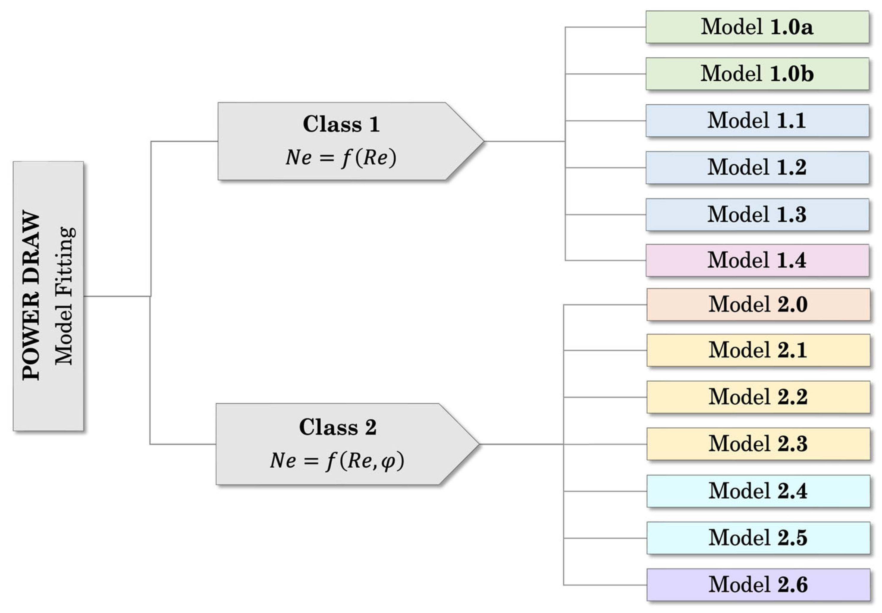
Figure 1. Fitting models for power consumption using dimensionless numbers. (Models following a similar pattern are highlighted using the same color. Class 1 color codes: green for single-region fitting, blue for multi-region fitting, and pink for non-regional, non-power-law-based fitting approach. Class 2 color codes: orange for single power-law fitting, yellow for multi-region fitting, light blue for fitting with logarithmically transformed variables, and purple for our novel fitting approach.) See text for further details.
Jpbi 02 00014 g001
Figure 2. Fitting of the Ne vs. Re data for three different φ values by (a) Model 1.0a, (b) Model 1.0b, (c) Model 1.1, (d) Model 1.2, (e) Model 1.3, and (f) Model 1.4. φ = 0.90 (orange, diamond), φ = 0.65 (cyan, star), and φ = 0.35 (navy, triangle).
Jpbi 02 00014 g002
Figure 3. Fitting of the Ne vs. Re using a single power-law correlation (Model 2.0) for three different bead filling ratios: φ = 0.90 (orange, diamond), φ = 0.65 (cyan, star), and φ = 0.35 (navy, triangle).
Jpbi 02 00014 g003
Figure 4. Fitting of the Ne vs. Re data for three different φ values by (a) Model 2.1, (b) Model 2.2, (c) Model 2.3, (d) Model 2.4, (e) Model 2.5, and (f) Model 2.6. φ = 0.90 (orange, diamond), φ = 0.65 (cyan, star), and φ = 0.35 (navy, triangle).
Jpbi 02 00014 g004
Figure 5. The equivalency plot (predicted Ne vs. experimental Ne) for the fit of Model 2.4 and Model 2.6 to Heidari et al. [30].
Jpbi 02 00014 g005
Table 1. Equations for the Class 1 models for Ne-Re correlations.
ModelEquationParameters
Model 1.0aLower transition region a: N e ( i ) = K ( i ) R e Y ( i )
Upper transition region b: model extension
Lower turbulent region c: constant value
Upper turbulent region d: constant value
K ( i ) , Y ( i )
Model 1.0bLower + upper transition region: N e ( i ) = K ( i ) R e Y ( i )
Lower turbulent region c: constant value
Upper turbulent region d: constant value
K ( i ) , Y ( i )
Model 1.1Lower transition region a: N e ( i ) = K 1 ( i ) R e Y 1 ( i )
Upper transition region b: N e ( i ) = K 2 ( i ) R e Y 2 ( i )
Lower turbulent region c: N e ( i ) = K 3 ( i ) R e Y 3 ( i )
Upper turbulent region d: N e ( i ) = K 4 ( i )
K 1 ( i ) , K 2 ( i ) , K 3 ( i ) , K 4 ( i ) ,
Y 1 ( i ) , Y 2 ( i ) , Y 3 ( i )
Model 1.2Lower transition region a: N e ( i ) = K ( i ) R e Y 1 ( i )
Upper transition region b: N e ( i ) = K ( i ) R e Y 2 ( i )
Lower turbulent region c: N e ( i ) = K ( i ) R e Y 3 ( i )
Upper turbulent region d: N e ( i ) = K ( i )
K ( i ) , Y 1 ( i ) , Y 2 ( i ) , Y 3 ( i )
Model 1.3Lower transition region a: N e ( i ) = K ( i ) R e Y 1 ( i )
Upper transition region b: N e ( i ) = K ( i ) R e Y 2 ( i )
Lower turbulent region c: N e ( i ) = K ( i ) R e Y 3 ( i )
Upper turbulent region d: N e ( i ) = K 4 ( i )
K ( i ) , K 4 ( i ) ,
Y 1 ( i ) , Y 2 ( i ) , Y 3 ( i )
Model 1.4 N e ( i ) = a 1 ( i ) R e a 2 ( i ) + a 3 ( i ) R e a 4 ( i ) a 5 ( i ) a 1 ( i ) , a 2 ( i ) , a 3 ( i ) , a 4 ( i ) , a 5 ( i )
a 1.2 × 10² < Re < 8 × 10³; b 8 × 10³ < Re < 3.5 × 10⁴; c 3.5 × 10⁴ < Re < 2 × 10⁵; d Re > 2 × 10⁵.
Table 2. Equations for the Class 2 models for NeReφ correlations.
ModelEquationParameters
Model 2.0 N e = K φ X R e Y K , X , Y
Model 2.1Lower transition region a: N e = K 1 φ X 1 R e Y 1
Upper transition region b: N e = K 2 φ X 2 R e Y 2
Lower turbulent region c: N e = K 3 φ X 3 R e Y 3
Upper turbulent region d: N e = K 4 φ X 4
K 1 , K 2 , K 3 , K 4 ,
X 1 , X 2 , X 3 , X 4
Y 1 , Y 2 , Y 3
Model 2.2Lower transition region a: N e = K φ X 1 R e Y 1
Upper transition region b: N e = K φ X 2 R e Y 2
Lower turbulent region c: N e = K φ X 3 R e Y 3
Upper turbulent region d: N e = K φ X 4
K ,
X 1 , X 2 , X 3 , X 4
Y 1 , Y 2 , Y 3
Model 2.3Lower transition region a: N e = K φ X 1 R e Y 1
Upper transition region b: N e = K φ X 2 R e Y 2
Lower turbulent region c: N e = K φ X 3 R e Y 3
Upper turbulent region d: N e = K 4 φ X 4
K , K 4
X 1 , X 2 , X 3 , X 4
Y 1 , Y 2 , Y 3
Model 2.4 l o g N e = a 0 + a 1 l o g R e + a 2 l o g φ + a 3 l o g R e 2 + a 4 l o g φ 2 + a 5 l o g R e l o g φ a 0 , a 1 , a 2 , a 3 , a 4 , a 5
Model 2.5 l o g N e = a 0 + a 1 l o g R e + a 2 l o g φ + a 3 l o g R e 2 + a 4 l o g φ 2 + a 5 l o g R e l o g φ + a 6 l o g R e 3 + a 7 l o g φ 3 + a 8 l o g R e 2 l o g φ + a 9 l o g φ 2 l o g R e a 0 , a 1 , a 2 , a 3 , a 4 ,
a 5 , a 6 , a 7 , a 8 , a 9
Model 2.6 N e = 1 l n ( a 1 R e a 2 + a 3 φ a 4 ) 2 a 1 , a 2 , a 3 , a 4
a 1.2 × 10² < Re < 8 × 10³; b 8 × 10³ < Re < 3.5 × 10⁴; c 3.5 × 10⁴ < Re < 2 × 10⁵; d Re > 2 × 10⁵.
Table 3. Parameter estimates and their standard errors based on fitting of Model 2.6 to the data of Kwade & Schwedes [22].
SSR aRMSE bR2
36.710.5910.990
ParameterEstimateSE c
a 1 1.27 × 1001.46 × 10−2
a 2 1.15 × 10−12.91 × 10−3
a 3 2.85 × 10−18.40 × 10−3
a 4 2.67 × 1002.79 × 10−1
a SSR: sum of squared residuals; b RMSE: root mean squared error; c SE: standard error.
Table 4. Parameter estimates and their standard errors based on fitting of Model 2.6 to Heidari et al. [30].
SSR aRMSE bR2
0.02210.04290.963
ParameterEstimateSE c
a 1 3.47 × 10516.63
a 2 1.96 × 1000.011
a 3 2.79 × 10−10.010
a 4 1.46 × 1000.174
a SSR: sum of squared residuals; b RMSE: root mean squared error; c SE: standard error.
Disclaimer/Publisher’s Note: The statements, opinions and data contained in all publications are solely those of the individual author(s) and contributor(s) and not of MDPI and/or the editor(s). MDPI and/or the editor(s) disclaim responsibility for any injury to people or property resulting from any ideas, methods, instructions or products referred to in the content.