Abstract
The accurate estimation of urban property values is a key challenge for appraisers, market participants, financial institutions, and urban planners. In recent years, machine learning (ML) techniques have emerged as promising tools for price forecasting due to their ability to model complex relationships among variables. However, their application raises two main critical issues: (i) the risk of overfitting, especially with small datasets or with noisy data; (ii) the interpretive issues associated with the “black box” nature of many models. Within this framework, this paper proposes a methodological approach that addresses both these issues, comparing the predictive performance of three ML algorithms—k-Nearest Neighbors (kNN), Random Forest (RF), and the Artificial Neural Network (ANN)—applied to the housing market in the city of Salerno, Italy. For each model, overfitting is preliminarily assessed to ensure predictive robustness. Subsequently, the results are interpreted using explainability techniques, such as SHapley Additive exPlanations (SHAPs) and Permutation Feature Importance (PFI). This analysis reveals that the Random Forest offers the best balance between predictive accuracy and transparency, with features such as area and proximity to the train station identified as the main drivers of property prices. kNN and the ANN are viable alternatives that are particularly robust in terms of generalization. The results demonstrate how the defined methodological framework successfully balances predictive effectiveness and interpretability, supporting the informed and transparent use of ML in real estate valuation.
1. Introduction
Accurately estimating the value of urban real estate is a highly relevant issue. This applies, first and foremost, to real estate market participants, but also to players in the banking and insurance sectors, where the asset can be a key collateral for the provision of loans or the definition of insurance coverage [1]. Rico-Juan and de La Paz [2] also highlight how housing price forecasting has relevance at the macroeconomic level, influencing both buyers in planning their investments and real estate companies. Indeed, the latter may choose to adopt different marketing strategies depending on whether the real estate market is in a period of growth or recession. Again, the reliable estimation of real estate values is essential for proper tax assessment and to assist planners in managing urban planning policies [3,4,5,6].
In recent decades, alongside the methodologies traditionally used in forecasting real estate values such as the Hedonic Price Model (HPM), techniques based on Artificial Intelligence (AI) and machine learning (ML) have rapidly gained popularity [7]. Assuming that the market value of a property depends on its characteristics, both intrinsic and extrinsic, hedonic regression emerges as one of the main tools for estimating marginal prices, which are the specific contribution of each property characteristic to the overall value of the property. ML and AI models have shown considerable potential in hedonic modeling, especially for predictive purposes [2]. Among the main advantages of these models, foremost is their ability to learn and model nonlinear relationships between variables, thus improving the predictive performance compared to those of the traditional models [3,4]. Although these techniques can provide more accurate predictions, their “black box” nature has raised concerns regarding their interpretability and transparency, casting questions about whether the decision-making process leading to the final prediction can be fully understood [8]. This issue is also addressed in RICS Valuation—Global Standards [9], which for the first time introduces specific guidelines on integrating AI into valuation processes. The document stresses the importance of preserving human professional judgment, while ensuring transparency for clients. Thus, the need to rigorously assess the quality, reliability, and traceability of the results generated by AI-based tools is highlighted, affirming the principle that the ultimate responsibility for evaluation remains with a qualified professional.
When the training dataset is insufficient in size relative to the complexity of the model, or contains a significant amount of irrelevant information — conditions frequently observed in real estate datasets — the phenomenon of overfitting may occur. In such cases, the machine learning algorithm tends to fit the training data too closely, or even memorize it, thereby undermining its ability to generalize effectively with unseen data.
The second issue is related to the nature of ML techniques, which, as noted above, return results that are spurious and often difficult to interpret [10]. According to Lorenz et al. [11], one solution is to limit the complexity of the models to ensure interpretability. An alternative is to examine the existing ML algorithms and “open up their results to establish interpretability.” In this regard, recent major advances in the explainability of ML models make them increasingly attractive, with important consequences for their interpretability, robustness, and ultimately reliability [12].
This paper proposes an innovative methodological approach aims to address both the issues outlined. Specifically, the predictive capabilities of three machine learning algorithms are compared: the Artificial Neural Network (ANN), Random Forest (RF), and k-Nearest Neighbors (k-NN). For each model, the presence of overfitting phenomena is preliminarily analyzed. Where such phenomena are found to be contained within acceptable limits, the forecast results are interpreted using explainability techniques.
This article is organized as follows: Section 2 proposes a critical review of the relevant literature. Section 3 outlines the defined methodological approach. In Section 4, the methodological approach is implemented with reference to the real estate market in the city of Salerno, Italy. Section 5 provides a critical evaluation of the results and a discussion of their implications. Finally, Section 6 concludes with a summary of the evidence that emerged and with suggestions for future elaboration.
2. State of Research
The origins of hedonic models can be traced to the pioneering work of Court [13], who first applied them to the automotive industry. Later, the studies by Lancaster [14] and Rosen [15] extended their use to the real estate context, stimulating extensive theoretical and empirical development. Analyses by Sheppard [16], Malpezzi [17], and Sirmans et al. [18] highlight the complexity and heterogeneity of issues arising in the use of this approach. According to Dubin [19], the real estate characteristics that most commonly influence the price formation mechanism include those that are (i) intrinsic or structural; (ii) locational; or (iii) neighborhood. The structural characteristics (i) include elements pertaining to the housing unit, such as the floor area, the age of a building, and the number of rooms. The locational ones (ii) refer to distance from points of interest, such as the city center or other relevant services. The neighborhood variables (iii) describe the surrounding socioeconomic context, including factors such as average income, crime, and characteristics of the urban environment. Because the locational and neighborhood components are often interrelated, it is common for them to be analyzed together and more generally referred to as extrinsic [20,21,22,23].
In recent years, the literature has focused heavily on the impact of the environmental, infrastructural, and social variables associated with urban location or context. For example, Ki and Jayantha [24] analyzed the impact of an urban regeneration intervention on property prices during the different phases of the project—before initiation, during construction, and after completion—showing significant increases in both the pre- and post-construction phases. Dumm et al. [25], Rouwendal et al. [26], and Jauregui et al. [27] have addressed the effects of proximity to bodies of water on property values. Further research has focused on distance from urban parks [28] and exposure to air pollution [29]. Zhang et al. [30] found a positive and statistically significant effect of urban greenery on nearby property values, with an increase of between 5 percent and 20 percent. Similarly, Jim and Chen [31] quantified the positive externalities associated with the presence of city parks, which provide recreational spaces and amenities that improve the environmental quality and well-being of residents.
The negative impact of environmental pressures, on the other hand, has been explored in depth by Chiarazzo et al. [32], who studied the case of Taranto (Italy), showing how proximity to industrial plants and related ecosystem disruptions are reflected in a decrease in property prices. In line with these results, Nesticò and La Marca [33] point out that the large urban area of Salerno is affected by the harmful effects of pollution-producing activities, with property depreciation that can reach up to 43 percent.
Finally, Zhang and Zheng [34] show that better air quality leads to higher housing prices, confirming how the housing market tends to reward better environmental settings.
In the field of infrastructure, Hoen et al. [35], Hoen and Atkinson-Palombo [36], and Wyman and Mothorpe [37] studied the impact of elements such as wind turbines and power lines on property valuation. Transportation accessibility, including highways and rail lines, has been analyzed by Chernobai et al. [38], Li [39] and Chin et al. [40], and Chakrabarti et al. [41].
Although the hedonic model based on multiple regression analysis (MRA) has long been the main forecasting tool in real estate, several scholars have pointed out its important limitations. It has been observed that MRA tends to return biased or underestimated estimates when the data have nonlinear relationships [42]. Given the complexity and dynamic nature of the real estate market, which is characterized by the simultaneous interaction of multiple heterogeneous variables, the need for more advanced predictive tools capable of capturing these relationships more accurately and effectively is increasingly emerging. Therefore, machine learning (ML) algorithms have been proposed as possible solutions to handle the linear and nonlinear relationships in a dataset where both categorical and numerical variables exist. According to Pérez-Rave et al. [43], although the parametric approach based on hedonic regression is widely used for inferential purposes, it is less effective when applied for predictive purposes. In contrast, in the field of machine learning, the focus has predominantly been on predictive capabilities, while inference has so far played a marginal role due to the often-opaque nature of the algorithms employed. In this context, ML models have emerged as promising tools for prediction, offering a superior performance over those of the traditional methods, especially in the presence of complex and nonlinear data structures.
In recent years, machine learning models based on Artificial Neural Networks (ANNs) have emerged as forerunners for improving the accuracy of real estate price prediction [44,45,46,47,48]. Numerous studies have shown that ANNs offer a superior performance compared to those of other traditional methods, standing out for their high accuracy in predictive estimates [49,50,51,52].
In the field of predictive modelling, several machine learning algorithms have distinguished themselves by their ability to learn from data and progressively refine their performance. Among them, techniques such as gradient tree boosting (GTB) [53], random forest regression (RFR) [54], and support vector regression (SVR) [55] have proven to be particularly effective, delivering highly accurate results. The literature on real estate confirms the effectiveness of these approaches. For example, studies such as those by Yoo et al. [56], Antipov and Pokryshevskaya [57], and Yao et al. [58] have focused on the performance of RFR. In contrast, Lam et al. [59] and Kontrimas and Verikas [60] explored the effectiveness of SVR. Boosting-based methods such as GTB have been analyzed by van Wezel et al. [61] and Kok et al. [62]. In addition, research by Zurada et al. [63] and Mayer et al. [64] compares the potential of different ML techniques. Again, Cajias et al. [65] show how such tools can be used effectively in market analysis and the management of real estate portfolios.
Two main gaps emerge from the literature. The first limitation found in the use of machine learning algorithms in the real estate context concerns the handling of overfitting, a phenomenon that is particularly evident when working with small datasets often consisting of a few hundred observations. In these cases, the algorithm tends to “overlearn” the training data, adapting not only to general patterns, but also to noise and anomalies in the data. This behavior leads to the loss of generalization ability, that is, a drastic reduction in predictive effectiveness when the model is applied to new or unseen data.
Empirical studies confirm this issue. For example, research conducted by Pérez-Rave et al. [43] highlights how machine learning models, while offering a strong predictive performance, can suffer from overfitting when applied to small sample sizes, thus compromising their ability to generalize to new data. Overfitting is a critical challenge, especially in areas such as real estate, where the availability of quality data may be limited and the inherent variability in markets is high. Although techniques exist to mitigate this risk—such as regularization, cross-validation, reducing model complexity, and increasing the dataset size through data augmentation techniques—their adoption is not always systematic in the existing literature, leaving room for improvement in the methodological approach [13,43].
Applications of machine learning (ML) are often criticized for their opaque nature, commonly described as a “black box” [66]. This is because predictive models generate accurate outcomes, but rarely offer clear explanations of the process that led to those outcomes. As Mayer et al. [64] note, ML models tend to prioritize prediction accuracy at the expense of transparency because they are designed to capture complex, nonlinear relationships within data, making it difficult to interpret their inner workings. While most studies on the use of ML to predict property prices have focused primarily on the predictive performance of the algorithms, less attention has been given to the explainability of these models. In fact, there are still few studies on ML that analyze the contribution of individual input variables to property price prediction.
Authors such as Chiarazzo et al. [32] suggest an approach to identify the most influential input variables, which consists of repeating the training process of the Artificial Neural Network, removing an input variable at each iteration. The importance of each variable is assessed by comparing the value of the coefficient of determination R obtained at the end of each training cycle. If a variable shows a significant change in the value of R upon its removal, this is interpreted as a signal of its significance in the predictive model.
Other scholars propose to complement or replace traditional sensitivity analysis with Explainable Artificial Intelligence (XAI) methodologies, which allow for the behavior of machine learning models to be interpreted more transparently [67,68,69,70,71]. Such approaches generally fall into two categories: global and local. Global approaches, such as Permutation Feature Importance (PFI), refer to the trained model. The rationale is to perform permutations on the value of each individual input variable and compare the variability in predictions. However, PFI can be affected by multicollinearity among variables, reducing its effectiveness in the presence of correlated features [68].
Among the local explainability approaches used to understand which variable features contribute most to prediction, Local Interpretable Model-Agnostic Explanation (LIME) and SHapley Additive exPlanations (SHAP) are emerging. For each input sample to be explained, LIME generates new samples of similar data, retrains the model, and compares the differences between the predictions generated from the original data samples and those generated randomly. However, the effectiveness of LIME can be affected by the choice of kernel and neighborhood size and may be unstable if the underlying model is highly nonlinear [67].
The SHAP approach, on the other hand, relies on the Shapley values obtained using the cooperative game theory to understand how much each input variable contributes to the model outcome. This approach provides both locally and globally consistent explanations, but can be computationally intensive, especially with complex models and many features [68,69,70].
Within this framework, this study aims to fill this gap by proposing a comparison of different machine learning (ML) models. This analysis will focus not only on predictive accuracy, but also on the interpretability of the predictions. The application focus will be the real estate market in the city of Salerno, with the aim of evaluating the effectiveness and transparency of predictive techniques in a real and specific context.
3. Methodology
The aim is to define a structured and replicable methodological framework that guides analysts in the use of machine learning (ML) algorithms for predicting urban real estate values, even in the presence of datasets limited to a few hundred observations. There are two key steps. The first consists in identifying potential overfitting phenomena. The second is to enhance the transparency of the result interpretation phase by leveraging Explainable Artificial Intelligence (XAI). These steps were structured in a replicable pipeline to ensure both predictive accuracy and model interpretability, even in data-constrained contexts.
In this work, we compare three machine learning algorithms widely used in the field of housing price prediction: the Artificial Neural Network (ANN), k-Nearest Neighbors (k-NN), and Random Forest (RF).
Among the Artificial Neural Networks, the Multilayer Perceptron (MLP) is one of the most widely adopted feedforward networks. It consists of one or more hidden layers in which each neuron is fully connected to the neurons in the preceding and succeeding layers. Each processing unit receives inputs from the previous layer, applies a nonlinear activation function (e.g., ReLU, Sigmoid, or Tanh), and transmits the result to the next layer, enabling the network to learn nonlinear representations of the data. The learning process occurs through gradient-based optimization algorithms, particularly the backpropagation technique combined with methods such as gradient descent (either standard or optimized variants like Adam). The objective is to minimize the cost function that quantifies the discrepancy between the predicted values and the observed ones. Thanks to its structure, the MLP neural network is capable of modelling complex and nonlinear relationships between the input and the output. However, its proper functioning requires careful architectural design (number of layers and number of neurons per layer) and the accurate tuning of training parameters (activation function, learning rate, and regularization techniques) to avoid overfitting phenomena, which may be critical when dealing with small-sized datasets [71].
The k-Nearest Neighbors (k-NN) algorithm is a supervised learning technique that bases the prediction of a value (or class) on the analysis of the k closest examples present in the training dataset. Proximity is measured using a distance metric, typically Euclidean distance. The underlying assumption of the model is that similar data tend to have similar responses. In the prediction phase, k-NN interpolates the output value by combining the values of the nearest neighbors. The key parameter of the algorithm is k, that is, the number of neighbors considered; an overly small value may lead to noisy models (overfitting), while an overly large value may introduce excessive generalization (underfitting) [72].
Random Forest (RF) is a supervised learning method based on an ensemble of decision trees. The central idea is to construct a multitude of trees, each trained on random samples of the dataset, and to aggregate their predictions to obtain a result that is more accurate and robust than that produced by a single tree. During the construction of each tree, each node is associated with a random subset of the available features to determine the optimal split, thus increasing the diversity among the trees. The main parameter is the number of generated trees, which affects both predictive performance and computational time. Random Forest is known for its ability to handle noisy and high-dimensional datasets [54].
The following section describes the proposed logical, operational steps useful for implementing and comparing these three ML algorithms.
- To improve clarity, this methodology is structured into sequential operational steps, each of which corresponds to a critical phase of model construction and evaluation. In each step, attention was paid not only to the theoretical underpinnings, but also to empirical implementation choices in order to make the approach reproducible and transparent. Moreover, the algorithms’ specific behavior with small datasets is discussed throughout, with practical considerations for scalability and generalization.
- Data Collection and Identification of Real Estate Features. This phase consists in the systematic acquisition of information relevant to the phenomenon under investigation, with the objective of ensuring the quality, completeness, and representativeness of the dataset. Particular attention was devoted to the identification of the most relevant explanatory variables, as well as to the verification of data consistency, the absence of outliers, and the management of potential missing values. Accurate data collection represents a necessary condition for ensuring the reliability of the subsequent modelling and analysis phases.
- Preliminary Feature Analysis and Data Normalization. Before implementing machine learning models, it is essential to conduct the preliminary analysis of features. This process includes the assessment of descriptive statistics, the evaluation of correlations between the independent variables and the target variable, and the identification of potential multicollinearity issues. This analysis helps researchers to select the most informative features, facilitating dimensionality reduction and improving model interpretability. Uninformative or redundant variables are excluded to limit noise and reduce the risk of overfitting, an especially critical concern when working with small datasets.Feature scaling is another fundamental step. Since many machine learning techniques—such as neural networks and distance-based models—are sensitive to the scale of variables, it is important to transform the features so they share comparable scales. Among the most commonly used techniques are standardization (z-score normalization), which transforms data to have zero mean and unit variance, and min-max normalization, which rescales values to a specific range, usually [0, 1]. These transformations not only promote algorithmic stability and faster convergence during training, but also help ensure that each variable contributes appropriately to the model’s learning process. In models such as neural networks, this can also prevent saturation of activation functions, while in k-NN, it ensures that features with larger numerical ranges do not disproportionately affect distance calculations.
- Parameter Tuning and Implementation of ML Algorithms. The proper configuration of machine learning algorithm parameters is fundamental to optimize the predictive performance and minimize the risk of overfitting, especially in contexts characterized by small-sized datasets. Regarding the Multilayer Perceptron (MLP), the critical parameters include the number of hidden layers and neurons per layer, the activation function (e.g., ReLU or Tanh), the learning rate, and the optimization strategy (e.g., Adam or SGD). For the k-Nearest Neighbors (k-NN) algorithm, the choice of the k parameter (number of neighbors considered) is essential, as is the type of distance metric used (e.g., Euclidean or Manhattan). For Random Forest, the most influential parameters include the number of trees in the forest, the maximum depth of the trees, and the maximum number of features considered at each split.Beyond their predictive performance, it is also relevant to consider the structural properties of the models and their behavior in different settings. Random Forest is an ensemble method based on decision trees, generally robust to noise, and relatively easy to tune, but its computational cost increases with the number of trees and the dataset size [54]. The k-Nearest Neighbors (kNN) algorithm, by contrast, is non-parametric and simple, but highly sensitive to the choice of kNN and suffers in scalability, as prediction requires computing distances to all training samples [72]. The Neural Network, while offering greater modeling flexibility, requires careful tuning of multiple hyperparameters (e.g., number of layers, neurons, and learning rate), and is prone to overfitting, especially on small datasets. However, it is the most scalable among the three; when applied to larger datasets, it can be trained efficiently using specialized hardware such as Graphics Processing Units (GPUs), which are designed to handle massive numerical computations in parallel [73]. This allows for neural networks to significantly reduce training time and handle increasingly large data volumes, making them particularly suitable for real-world applications with growing datasets [74].
- Analysis and Validation of Results. The performance evaluation of the algorithms was conducted through the analysis of the main regression metrics, in particular the coefficient of determination (R2), the mean squared error (MSE), and the mean absolute error (MAE). These metrics were estimated according to the following formulations:
- These metrics were calculated both for the training set and through a k-fold cross-validation procedure in order to obtain more reliable estimates of the models’ generalization capability.
- Cross-validation involves partitioning the dataset into k subsets (folds), which are cyclically used for training and validation. This approach makes it possible to assess performance across multiple data splits, reducing the impact of specific data configurations. It also helps to detect potential overfitting phenomena, which become evident when there are significant discrepancies between the metrics computed on the training and validation sets.
- To enhance the transparency of model comparison, all the performance metrics were aggregated and summarized, allowing for the clear evaluation of the strengths and limitations of each algorithm. Quantitative analysis was complemented by model interpretation techniques, discussed in the following sections, which support a deeper understanding of the influence of individual features on the predictions.
- 5.
- Model Explainability and Feature Importance. To enhance the interpretability of the employed machine learning models, analysis was supplemented with techniques from Explainable Artificial Intelligence (XAI).Among these, SHapley Additive exPlanations (SHAP) values were calculated to quantify the marginal impact of each input feature on the model’s predictions. SHAP assigns an importance score to each feature by considering all the possible combinations of features, thus providing a theoretically grounded and locally consistent explanation of the model’s behavior.In addition, a Permutation Feature Importance technique was used to assess how much the prediction error increases when a single feature’s values are randomly shuffled. This disrupts the relationship between that feature and the target, allowing for a direct estimate of its contribution to model performance.These techniques—supported through the case study by empirical examples and visualizations—enable a better understanding of the “black box” nature of complex algorithms. They also support the decision-making process in urban real estate analysis by highlighting which features most influence property values.
4. Case Study
4.1. Data Collection and Identification of Real Estate Features
The sample under analysis consists of 210 urban residential properties sold in the city of Salerno during the 2022–2024 period. With a population of approximately 126,000 inhabitants, Salerno is the second-most-populous urban center in the Campania Region and one of the main economic and territorial hubs in Southern Italy. Information regarding the real estate transactions was collected through direct collaboration with leading local real estate agencies, which provided access to the data via the property management software “Asset Pricing Venduto” used for storing property characteristics and transaction details.
From a territorial perspective, the Municipality of Salerno is divided according to the classification of the Osservatorio del Mercato Immobiliare (OMI) of the Italian Revenue Agency into 16 OMI zones. These subdivisions represent urban areas that are homogeneous in terms of building typology, socioeconomic profile, and infrastructure and serve as a standardized basis for official property valuation data collection.
The dataset used in this study includes properties located in four distinct OMI zones (B10, B11, B12, C3, and R11), all situated within or near the city center, in order to ensure a relatively high degree of spatial homogeneity and the comparability of observations.
The independent variables included in analysis were selected based on data availability and territorial consistency, distinguishing between intrinsic property features and extrinsic characteristics related to the urban context.
The intrinsic features considered are as follows:
- Commercial surface (SUR), expressed in square meters;
- The floor level of the residential unit (FLOOR), expressed as a numerical level;
- The state of maintenance (CONS), an ordinal categorical variable with values coded as 1 = “to be renovated”, 3 = “good”, or 5 = “excellent”;
- The presence of an elevator (LIFT), a binary (dummy) variable (1 = present, 0 = absent).
The extrinsic features were identified based on targeted territorial analysis and refer to the proximity of the property to key infrastructure. Values are expressed as estimated travel time (in minutes) under free-flow traffic conditions:
- T1—Travel time from each property to the central railway station, located near the historic center and representing the main urban hub. This rendered the inclusion of a “distance to city center” variable unnecessary, thereby avoiding informational redundancy and multicollinearity issues;
- T2—Travel time to the commercial port;
- T3—Travel time to the main highway entrance (Fratte interchange).
Table 1 presents the main descriptive statistics of the dataset, offering a quantitative overview that helps contextualize the variables used in the predictive model. Figure 1 shows the geolocation of the properties under study and of the main reference services, highlighting the spatial distribution of the data.

Table 1.
Descriptive statistics of the dataset.
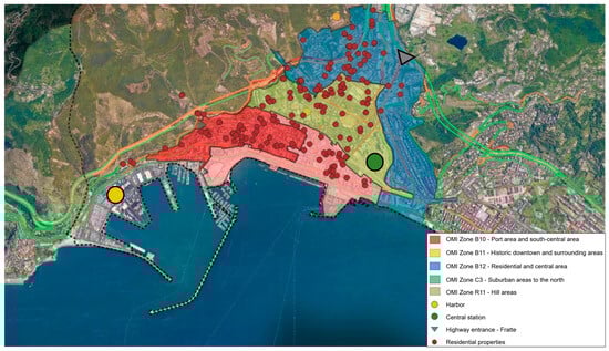
Figure 1.
Geolocation of real estate data and key services and attractions.
4.2. Preliminary Feature Analysis and Data Normalization
Correlation analysis yielded the following key results:
- The variable SUR (commercial surface) exhibits a strong positive correlation with the price (coefficient = 0.841);
- The presence of an elevator (LIFT) is moderately and positively correlated with the price (0.336), indicating that this feature significantly contributes to property value;
- The variable FLOOR shows a weak correlation with the price (0.231), while CONS (state of conservation) presents an almost null correlation (−0.039). Nevertheless, both these characteristics are considered relevant from an appraisal perspective and were therefore retained in analysis;
- The variables T1, T2, and T3—travel times to the railway station, the commercial port, and the main highway entrance, respectively, exhibit moderately negative correlations with price (T1 = −0.549; T2 = −0.127; and T3 = −0.310).
- Moderate correlations were also observed among some of the independent variables, specifically between T2 and T1 (0.466), and between T3 and T2 (0.645). These relationships warrant caution during modeling to avoid multicollinearity issues.
In summary, the confirms the presence of expected relationships between the price and certain explanatory variables, while also highlighting the importance of adopting methods capable of capturing nonlinear effects and variable interactions. Table 2 shows the correlation analysis.
Table 2.
Correlation analysis.
Feature normalization is a fundamental step in certain machine learning algorithms, as it ensures comparability among variables expressed on different scales.
In particular, both the k-Nearest Neighbors (k-NN) and Multilayer Perceptron (MLP) neural networks require normalization. The former relies on Euclidean distance metrics, where variables on different scales can distort distance calculations [75]. The latter employs numerical optimization methods such as gradient descent, which are sensitive to the scale of input data [76].
In contrast, tree-based algorithms such as Random Forest do not require normalization, since the tree-splitting criteria depend solely on the ordering of values rather than their absolute magnitudes [54].
Accordingly, in the preprocessing phase, feature normalization was applied to the k-NN and MLP models, but not to Random Forest.
This study adopts a standardization procedure (zero-mean and unit-variance scaling) for both the k-NN and MLP models. As discussed by James et al. [77], standardization preserves the original distribution of the data, reduces the influence of outliers, and improves numerical stability during model training. This approach also enables the more accurate interpretation of the weights learned by the neural network and the more equitable assessment of distances in similarity-based models.
4.3. Parameter Tuning and Implementation of ML Algorithms
For the prediction of real estate prices, three machine learning models were implemented, k-Nearest Neighbors (kNN), Random Forest, and Multilayer Perceptron (MLP), using the Orange platform. The parameters of the models were iteratively optimized to maximize the predictive performance, specifically the coefficient of determination (R2).
In the kNN model, the number of neighbors was set to five using Euclidean distance and uniform weights, which resulted in a good balance between complexity and generalization ability. For the Random Forest model, the number of trees was set to 100, a choice that ensured sufficient stability in predictions without excessively compromising training time; the depth of the trees was limited to three levels to avoid overfitting. Finally, the neural network was configured with two hidden layers, each containing 132 neurons, ReLU activation, and the Adam optimizer. A regularization term with α = 10 was applied to improve generalization, and the maximum number of iterations was set to 5000 to ensure the adequate convergence of the model.
The choice of these parameters was driven by an empirical tuning process aimed at comparing the different configurations, and therefore selecting those that offer the best performance with the considered dataset.
The results indicate that in most cases, the prices estimated by the three models are close to the actual observed values, suggesting the ability of each model to capture the relationship between the characteristics of the properties and their market price. However, in some cases, significant discrepancies were observed, with visible deviations between the actual value and the predicted ones. These deviations may be due to the presence of outliers (properties with atypical characteristics) or the models’ difficulty in generalizing correctly on certain portions of the dataset. The predicted values for each property by each model are reported in Appendix A.
4.4. Analysis and Validation of Results
To evaluate the performance of the real estate price prediction models, both a cross-validation approach (20-fold) and the direct assessment of the training data were implemented. Cross-validation estimates the models’ generalization ability, while the evaluation on the training data helps detect potential overfitting. Given the relatively small dataset size, a comparison between the metrics obtained from these two methods is particularly relevant.
The results are presented in Table 3 and Table 4, which show the evaluation metrics for the three models using cross-validation and training data tests, respectively. The analyses reveal, first and foremost, that the Random Forest achieves a superior performance compared to those of the other models, with an R2 of 0.956 and a Mean Absolute Percentage Error (MAPE) of 0.110 on the training data, indicating a very prominent predictive ability. However, it was observed that Random Forest tends to overfit the training data, as evidenced by the discrepancy in the metrics between training and cross-validation (R2 = 0.842, MAPE = 0.205).
Table 3.
Evaluation metrics (cross-validation with k = 20).
Table 4.
Evaluation metrics (test on training data).
In contrast, the kNN and Neural Network models achieve R2 values of 0.843 and 0.819 on the training data, respectively, while in cross-validation, their R2 values decrease to 0.715 and 0.758. The kNN model exhibits the largest variation between training and validation, while the neural network shows a more limited difference, indicating a more balanced trade-off between bias and variance and less overfitting. However, both these models are less accurate in absolute terms compared to Random Forest, but demonstrate greater stability between training and validation.
It is important to note that neural networks, due to their high flexibility and large number of trainable parameters, are particularly sensitive to overfitting when trained on limited datasets. In such conditions, the model may learn specific patterns and noise from the training set rather than general trends, reducing its ability to generalize to new data. This behavior reinforces the need for rigorous validation strategies such as cross-validation, and possibly for regularization techniques. While in this case the neural network did not overfit severely, its performance reflects the typical vulnerability of complex models to data scarcity.
In summary, the kNN and Neural Network models exhibit less overfitting compared to what was observed in Random Forest. However, the latter remains the model with the best overall performance during the training phase. In general terms, these results confirm the validity of the tuning procedure adopted and the effectiveness of the selected models for predicting property values. Indeed, in a context with limited data, a certain degree of overfitting can be considered acceptable, especially when (i) the gap between training and validation is not excessive; and (ii) the metrics in cross-validation (CV) remain high [78]. The results are, therefore, in line with what has been specified in the relevant literature. Authors such as Hastie, Tibshirani, and Friedman [79] emphasize that with smaller datasets, more flexible models—such as Random Forest and the ANN—tend to overfit the data, but if the performance in validation remains good, overfitting can be tolerated.
Thus, considering both the absolute metrics and the generalization ability, Random Forest emerges as the best model among those analyzed. Despite exhibiting moderate overfitting, its performance in validation remains superior to the other approaches, making it the most effective choice for predicting real estate values in this context.
4.5. Model Explainability and Feature Importance
This study on feature importance and the explainability of results was specifically implemented for the Random Forest model, as it provided the best overall performance across all the evaluation metrics (MSE, RMSE, MAE, MAPE, and R2).
Figure 2 presents a beeswarm plot based on SHapley Additive exPlanation (SHAP) values, an interpretability method derived from Shapley’s game theory. The SHAP values highlight the contribution of each variable to the model’s prediction. Each point represents an observation, colored according to the variable’s value (blue = low; red = high), while the position on the horizontal axis shows the impact of the variable on the predicted value.

Figure 2.
Beeswarm plot based on SHAP values for Random Forest model.
Figure 3 shows the importance of the input variables according to the Permutation Feature Importance method, which measures the reduction in predictive performance (specifically R2) when the value of a variable is randomly permuted. A greater reduction indicates the increased relevance of the predictor.
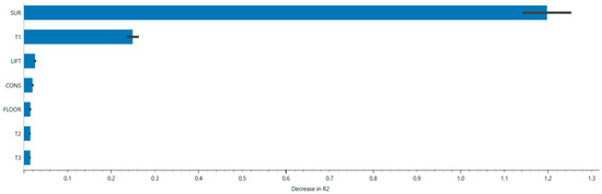
Figure 3.
Permutation feature importance for Random Forest model.
To assess the statistical significance of the key variables SUR and T1, we performed a permutation test. This involved randomly shuffling the values of each variable multiple times to break their association with the target variable and measuring the resulting decrease in model performance (R2). By comparing the observed decrease to the distribution of decreases obtained under random permutations, we confirmed that the impact of SUR and T1 on the model is statistically significant (p < 0.01). This confirms the robustness of their contribution to property value prediction.
Both the approaches converge in identifying the variables SUR (commercial surface) and T1 (distance to the station) as the most influential in determining the predicted value of the model. In particular, SUR shows a very marked and consistent impact in both analyses, confirming its centrality in estimating property values. Other variables, such as CONS (conservation state), T2 (time to highway entrance), LIFT (elevator presence), and T3 (time to the port), exert progressively more marginal influences.
5. Discussion
For the prediction of real estate prices, three models were implemented and compared: k-Nearest Neighbors (kNN), Random Forest, and the Multi-Layer Artificial Neural Network. These models were evaluated using both 20-fold cross-validation and a test conducted on the same training set to detect any potential overfitting in a dataset of limited size [77]. In cross-validation, Random Forest achieved a coefficient of determination (R2) of 0.842, while on the training set, its R2 increased to 0.956, suggesting a slight, but contained overfitting due to the ensemble mechanism [54]. The kNN, configured with k = 5 and Euclidean distance, recorded an R2 value of 0.715 in cross-validation and 0.843 on the training set, reflecting its sensitivity to noise, but also an ability to generalize [72]. The Neural Network, equipped with two hidden layers of 132 neurons each, the ReLU activation function, and the Adam optimizer, showed R2 = 0.758 in cross-validation and R2 = 0.819 on the training set, confirming that greater complexity can still provide a good performance if supported by proper regularization [76].
To deepen the understanding of the Random Forest model, interpretability analyses were conducted using SHAP (SHapley Additive exPlanations) and Permutation Feature Importance (PFI). The SHAP values helped identify the property area (SUR) and the distance from the station (T1) as the main drivers of the predicted value. The beeswarm plots show that an increase in SUP tends to positively influence the predicted price, while a greater distance from the station has a negative impact. PFI analysis confirms these results; the random permutation of SUP and T1 values leads to a significant deterioration in predictive performance (in terms of R2), further confirming their centrality in the model.
Furthermore, a statistical significance assessment using permutation tests was performed on SUR and T1. By repeatedly shuffling the values of each variable and measuring the impact on model performance, the test confirmed that SUR and T1 are statistically significant (p < 0.01). This additional analysis reinforces the robustness of the conclusions regarding these key predictors in property value estimation.
Overall, all three models are suitable for the proposed application. The Random Forest model offers the best overall performance, while providing good interpretability through feature importance analysis. The kNN and Neural Network models represent valid alternatives, particularly robust in terms of generalization.
While the current dataset has generated meaningful insights into model behavior, some limitations remain due to its relatively small size. Future developments could benefit from the construction of a larger and more diverse dataset, which would strengthen the statistical robustness of the evaluation metrics reported in Table 3 and Table 4. This would also enable more reliable training–test splits and better generalization assessments.
6. Conclusions
This study highlights the potential of machine learning techniques for predicting urban real estate values, even when the initial dataset consist of only a few hundred data points. Specifically, it proposes an integrated approach, combining predictive accuracy evaluations with model interpretability tools. The results show that Random Forest is particularly well-suited for this task due to its ability to handle complex relationships between variables. Compared to the kNN and ANN models, Random Forest achieves a superior performance in terms of R2, MSE, RMSE, MAE, and MAPE, confirming the robustness of ensemble learning in complex regression scenarios.
In summary, Random Forest outperformed the other models in all the metrics (R2, MSE, RMSE, MAE, and MAPE), while kNN and the ANN offered acceptable generalization performances. All the models showed some degree of overfitting, reinforcing the importance of cross-validation when working with small datasets. Specifically, the models performed better on the training data than during cross-validation, confirming the risk of overfitting in limited sample contexts.
The adoption of interpretability techniques, such as SHAP and Permutation Feature Importance, helps to overcome, at least partially, the “black box” problem by identifying the real estate characteristics most influential on prices. In particular, the commercial surface (SUR) and the distance from the train station (T1) emerged as the key determinants, showing how the property price is strongly influenced by both intrinsic and extrinsic variables. This type of analysis not only provides greater transparency for the models, but also offers valuable insights for decision-making strategies by investors, real estate developers, and public administrations.
From a professional perspective, these findings offer actionable guidance; Random Forest can be applied as a reliable and interpretable tool for real estate valuation in urban contexts, particularly when working with heterogeneous and limited data. Identifying key drivers such as surface area and accessibility helps inform investment strategies, urban planning decisions, and policy development by public authorities.
Despite the promising results, this study also points out some limitations related to the relatively small size of the dataset and the potential variability in results across different real estate markets. Future research could expand the proposed approach to larger and more diverse datasets, incorporate additional explainability techniques, and explore the effectiveness of more advanced ML models—such as Gradient Boosting Machines and deep neural networks—with the aim of further enhancing both predictive accuracy and model interpretability.
Author Contributions
Conceptualization, G.M. and A.N.; methodology, G.M. and A.N.; software, G.M. and A.N.; validation, G.M. and A.N.; formal analysis, G.M. and A.N.; investigation, G.M. and A.N.; resources, G.M. and A.N.; data curation, G.M. and A.N.; writing—original draft preparation, G.M.; writing—review and editing, G.M. and A.N.; visualization, G.M. and A.N.; supervision, G.M. and A.N.; project administration, A.N.; funding acquisition, A.N. All authors have read and agreed to the published version of the manuscript.
Funding
This research received no external funding.
Institutional Review Board Statement
Not applicable.
Informed Consent Statement
Not applicable.
Data Availability Statement
The raw data supporting the conclusions of this article will be made available by the authors on request.
Conflicts of Interest
The authors declare no conflicts of interest.
Abbreviations
The following abbreviations are used in this manuscript:
| ANN | Artificial Neural Network |
| MLP | Multilayer Perceptron |
| K-NN | k-Nearest Neighbors (k-NN) |
| RF | Random Forest |
Appendix A
Table A1.
Previsione dei prezzi degli immobili con i tre modelli: ANN, RF, and k-NN.
Table A1.
Previsione dei prezzi degli immobili con i tre modelli: ANN, RF, and k-NN.
| PRICE [EUR] | FORECAST kNN [EUR] | Δ [%] | FORECAST ANN [EUR] | Δ [%] | FORECAST RF [EUR] | Δ [%] |
|---|---|---|---|---|---|---|
| 80,000 | 108,400 | 35.50% | 93,948 | 17.44% | 85,161 | 6.45% |
| 108,700 | 114,740 | 5.56% | 114,291 | 5.14% | 104,010 | −4.31% |
| 80,000 | 73,400 | −8.25% | 74,558 | −6.80% | 78,567 | −1.79% |
| 70,000 | 99,000 | 41.43% | 68,098 | −2.72% | 89,727 | 28.18% |
| 80,000 | 83,600 | 4.50% | 72,398 | −9.50% | 80,943 | 1.18% |
| 60,000 | 114,000 | 90.00% | 121,909 | 103.18% | 81,179 | 35.30% |
| 80,000 | 104,000 | 30.00% | 110,597 | 38.25% | 76,775 | −4.03% |
| 145,000 | 114,000 | −21.38% | 130,780 | −9.81% | 132,235 | −8.80% |
| 145,000 | 114,000 | −21.38% | 130,780 | −9.81% | 132,235 | −8.80% |
| 145,000 | 140,400 | −3.17% | 149,164 | 2.87% | 144,391 | −0.42% |
| 85,000 | 114,740 | 34.99% | 118,509 | 39.42% | 99,207 | 16.71% |
| 210,000 | 239,000 | 13.81% | 215,798 | 2.76% | 220,497 | 5.00% |
| 110,000 | 114,740 | 4.31% | 135,883 | 23.53% | 130,908 | 19.01% |
| 130,000 | 114,000 | −12.31% | 140,584 | 8.14% | 142,197 | 9.38% |
| 90,000 | 114,000 | 26.67% | 117,826 | 30.92% | 87,102 | −3.22% |
| 110,000 | 139,400 | 26.73% | 150,960 | 37.24% | 121,085 | 10.08% |
| 190,000 | 204,400 | 7.58% | 205,386 | 8.10% | 194,307 | 2.27% |
| 110,000 | 131,200 | 19.27% | 95,357 | −13.31% | 116,554 | 5.96% |
| 60,000 | 90,400 | 50.67% | 67,953.9 | 13.26% | 63,920 | 6.53% |
| 160,000 | 167,000 | 4.38% | 168,224 | 5.14% | 157,929 | −1.29% |
| 200,000 | 132,600 | −33.70% | 143,976 | −28.01% | 180,599 | −9.70% |
| 270,000 | 219,000 | −18.89% | 275,874 | 2.18% | 272,889 | 1.07% |
| 180,000 | 202,200 | 12.33% | 206,213 | 14.56% | 193,001 | 7.22% |
| 250,000 | 188,000 | −24.80% | 259,065 | 3.63% | 249,730 | −0.11% |
| 250,000 | 202,200 | −19.12% | 232,110 | −7.16% | 250,650 | 0.26% |
| 70,000 | 150,400 | 114.86% | 150,457 | 114.94% | 98,869.2 | 41.24% |
| 110,000 | 105,140 | −4.42% | 111,140 | 1.04% | 100,374 | −8.75% |
| 150,000 | 140,400 | −6.40% | 151,924 | 1.28% | 151,441 | 0.96% |
| 130,000 | 179,000 | 37.69% | 146,059 | 12.35% | 126,966 | −2.33% |
| 60,000 | 90,400 | 50.67% | 67,953.9 | 13.26% | 63,919.6 | 6.53% |
| 300,000 | 266,000 | −11.33% | 281,678 | −6.11% | 263,758 | −12.08% |
| 250,000 | 273,000 | 9.20% | 322,411 | 28.96% | 267,973 | 7.19% |
| 630,000 | 570,000 | −9.52% | 565,441 | −10.25% | 583,548 | −7.37% |
| 195,000 | 183,000 | −6.15% | 160,885 | −17.49% | 179,937 | −7.72% |
| 137,000 | 142,200 | 3.80% | 154,629 | 12.87% | 140,712 | 2.71% |
| 145,000 | 142,200 | −1.93% | 150,055 | 3.49% | 140,091 | −3.39% |
| 110,000 | 79,000 | −28.18% | 107,878 | −1.93% | 112,020 | 1.84% |
| 125,000 | 142,200 | 13.76% | 135,305 | 8.24% | 126,165 | 0.93% |
| 270,000 | 157,000 | −41.85% | 227,086 | −15.89% | 270,670 | 0.25% |
| 140,000 | 142,200 | 1.57% | 164,891 | 17.78% | 163,739 | 16.96% |
| 360,000 | 390,000 | 8.33% | 339,014 | −5.83% | 368,093 | 2.25% |
| 370,000 | 297,600 | −19.57% | 319,229 | −13.72% | 321,956 | −12.98% |
| 210,000 | 241,400 | 14.95% | 179,669 | −14.44% | 234,027 | 11.44% |
| 170,000 | 183,000 | 7.65% | 160,885 | −5.36% | 179,937 | 5.85% |
| 300,000 | 301,000 | 0.33% | 343,257 | 14.42% | 313,243 | 4.41% |
| 350,000 | 253,000 | −27.71% | 223,853 | −36.04% | 273,276 | −21.92% |
| 285,000 | 301,000 | 5.61% | 331,194 | 16.21% | 308,260 | 8.16% |
| 205,000 | 253,000 | 23.41% | 288,726 | 40.84% | 241,015 | 17.57% |
| 310,000 | 468,000 | 50.97% | 378,547 | 22.11% | 317,115 | 2.30% |
| 297,000 | 313,400 | 5.52% | 385,094 | 29.66% | 322,606 | 8.62% |
| 630,000 | 548,000 | −13.02% | 579,595 | −8.00% | 572,921 | −9.06% |
| 225,000 | 334,000 | 48.44% | 236,428 | 5.08% | 220,256 | −2.11% |
| 485,000 | 501,000 | 3.30% | 503,263 | 3.77% | 529,233 | 9.12% |
| 395,000 | 311,000 | −21.27% | 406,059 | 2.80% | 437,196 | 10.68% |
| 395,000 | 329,400 | −16.61% | 432,239 | 9.43% | 444,044 | 12.42% |
| 190,000 | 242,400 | 27.58% | 277,559 | 46.08% | 220,896 | 16.26% |
| 280,000 | 273,000 | −2.50% | 322,411 | 15.15% | 267,973 | −4.30% |
| 510,000 | 395,000 | −22.55% | 360,804 | −29.25% | 468,166 | −8.20% |
| 540,000 | 468,000 | −13.33% | 485,700 | −10.06% | 514,953 | −4.64% |
| 253,000 | 297,600 | 17.63% | 311,723 | 23.21% | 268,299 | 6.05% |
| 550,000 | 467,000 | −15.09% | 554,914 | 0.89% | 578,320 | 5.15% |
| 540,000 | 409,400 | −24.19% | 385,101 | −28.69% | 476,620 | −11.74% |
| 595,000 | 546,000 | −8.24% | 592,184 | −0.47% | 592,950 | −0.34% |
| 600,000 | 468,000 | −22.00% | 484,904 | −19.18% | 545,309 | −9.12% |
| 247,000 | 234,400 | −5.10% | 200,373 | −18.88% | 224,812 | −8.98% |
| 83,000 | 86,800 | 4.58% | 92,811 | 11.82% | 74,813.4 | −9.86% |
| 245,000 | 202,200 | −17.47% | 275,292 | 12.36% | 308,441 | 25.89% |
| 310,000 | 278,000 | −10.32% | 286,696 | −7.52% | 294,794 | −4.91% |
| 440,000 | 346,000 | −21.36% | 367,109 | −16.57% | 434,041 | −1.35% |
| 210,000 | 208,000 | −0.95% | 194,739 | −7.27% | 218,565 | 4.08% |
| 255,000 | 239,000 | −6.27% | 243,428 | −4.54% | 272,906 | 7.02% |
| 430,000 | 294,000 | −31.63% | 279,290 | −35.05% | 369,038 | −14.18% |
| 430,000 | 365,400 | −15.02% | 316,203 | −26.46% | 410,311 | −4.58% |
| 130,000 | 147,000 | 13.08% | 109,564 | −15.72% | 141,632 | 8.95% |
| 400,000 | 370,000 | −7.50% | 361,857 | −9.54% | 425,829 | 6.46% |
| 130,000 | 147,000 | 13.08% | 101,520 | −21.91% | 137,736 | 5.95% |
| 480,000 | 468,000 | −2.50% | 399,573 | −16.76% | 442,715 | −7.77% |
| 410,000 | 399,600 | −2.54% | 347,779 | −15.18% | 373,773 | −8.84% |
| 620,000 | 494,000 | −20.32% | 530,554 | −14.43% | 529,780 | −14.55% |
| 200,000 | 200,000 | 0.00% | 218,388 | 9.19% | 176,664 | −11.67% |
| 75,000 | 85,400 | 13.87% | 82,062.5 | 9.42% | 81,926.1 | 9.23% |
| 135,000 | 145,200 | 7.56% | 225,320 | 66.90% | 141,406 | 4.75% |
| 152,000 | 147,200 | −3.16% | 146,660 | −3.51% | 138,750 | −8.72% |
| 125,000 | 107,800 | −13.76% | 120,831 | −3.34% | 119,518 | −4.39% |
| 152,000 | 147,200 | −3.16% | 154,788 | 1.83% | 138,559 | −8.84% |
| 123,000 | 107,800 | −12.36% | 114,077 | −7.25% | 102,653 | −16.54% |
| 108,000 | 107,800 | −0.19% | 114,077 | 5.63% | 102,653 | −4.95% |
| 68,000 | 107,800 | 58.53% | 114,077 | 67.76% | 102,653 | 50.96% |
| 79,000 | 98,600 | 24.81% | 107,588 | 36.19% | 90,856.7 | 15.01% |
| 175,000 | 154,000 | −12.00% | 168,157 | −3.91% | 163,857 | −6.37% |
| 86,000 | 123,800 | 43.95% | 96,747.7 | 12.50% | 125,917 | 46.42% |
| 125,000 | 109,800 | −12.16% | 104,898 | −16.08% | 111,679 | −10.66% |
| 125,000 | 136,800 | 9.44% | 94,589.4 | −24.33% | 127,295 | 1.84% |
| 150,000 | 147,200 | −1.87% | 163,353 | 8.90% | 151,596 | 1.06% |
| 30,000 | 81,600 | 172.00% | 96,067.3 | 220.22% | 72,353.9 | 141.18% |
| 200,000 | 150,600 | −24.70% | 181,959 | −9.02% | 175,931 | −12.03% |
| 50,000 | 157,000 | 214.00% | 202,763 | 305.53% | 134,384 | 168.77% |
| 125,000 | 109,800 | −12.16% | 128,623 | 2.90% | 119,008 | −4.79% |
| 395,000 | 372,000 | −5.82% | 376,240 | −4.75% | 423,526 | 7.22% |
| 200,000 | 166,600 | −16.70% | 154,306 | −22.85% | 171,777 | −14.11% |
| 350,000 | 295,800 | −15.49% | 259,384 | −25.89% | 341,387 | −2.46% |
| 180,000 | 179,600 | −0.22% | 190,652 | 5.92% | 177,848 | −1.20% |
| 340,000 | 362,000 | 6.47% | 340,046 | 0.01% | 366,164 | 7.70% |
| 115,000 | 107,800 | −6.26% | 114,077 | −0.80% | 102,653 | −10.74% |
| 180,000 | 147,000 | −18.33% | 130,446 | −27.53% | 165,857 | −7.86% |
| 145,000 | 86,000 | −40.69% | 67,207.2 | −53.65% | 120,231 | −17.08% |
| 430,000 | 252,000 | −41.40% | 244,341 | −43.18% | 368,123 | −14.39% |
| 48,000 | 75,600 | 57.50% | 73,468.2 | 53.06% | 69,561.5 | 44.92% |
| 112,000 | 98,000 | −12.50% | 127,750 | 14.06% | 105,960 | −5.39% |
| 48,000 | 100,600 | 109.58% | 103,889 | 116.44% | 96,305 | 100.64% |
| 112,000 | 100,600 | −10.18% | 103,889 | −7.24% | 96,305 | −14.01% |
| 108,000 | 100,600 | −6.85% | 79,238.1 | −26.63% | 96,606.4 | −10.55% |
| 290,000 | 249,000 | −14.14% | 232,599 | −19.79% | 262,379 | −9.52% |
| 265,000 | 278,000 | 4.91% | 284,160 | 7.23% | 291,125 | 9.86% |
| 130,000 | 170,600 | 31.23% | 122,418 | −5.83% | 133,624 | 2.79% |
| 175,000 | 228,600 | 30.63% | 149,479 | −14.58% | 166,048 | −5.12% |
| 440,000 | 303,000 | −31.14% | 372,791 | −15.27% | 402,736 | −8.47% |
| 260,000 | 249,000 | −4.23% | 257,127 | −1.11% | 262,753 | 1.06% |
| 180,000 | 230,000 | 27.78% | 225,035 | 25.02% | 196,373 | 9.10% |
| 400,000 | 252,600 | −36.85% | 345,968 | −13.51% | 400,122 | 0.03% |
| 365,000 | 388,000 | 6.30% | 319,215 | −12.54% | 376,104 | 3.04% |
| 230,000 | 239,000 | 3.91% | 215,798 | −6.17% | 220,497 | −4.13% |
| 190,000 | 183,600 | −3.37% | 149,998 | −21.05% | 178,201 | −6.21% |
| 365,000 | 490,000 | 34.25% | 595,442 | 63.13% | 402,845 | 10.37% |
| 128,000 | 183,600 | 43.44% | 155,804 | 21.72% | 141,131 | 10.26% |
| 165,000 | 156,600 | −5.09% | 167,773 | 1.68% | 164,117 | −0.54% |
| 510,000 | 471,000 | −7.65% | 451,773 | −11.42% | 489,513 | −4.02% |
| 240,000 | 164,000 | −31.67% | 213,914 | −10.87% | 234,672 | −2.22% |
| 265,000 | 259,000 | −2.26% | 308,548 | 16.43% | 296,873 | 12.03% |
| 295,000 | 277,000 | −6.10% | 271,813 | −7.86% | 284,468 | −3.57% |
| 370,000 | 349,000 | −5.68% | 341,544 | −7.69% | 384,913 | 4.03% |
| 190,000 | 212,000 | 11.58% | 202,866 | 6.77% | 188,883 | −0.59% |
| 195,000 | 184,800 | −5.23% | 232,662 | 19.31% | 208,129 | 6.73% |
| 318,000 | 277,000 | −12.89% | 293,566 | −7.68% | 285,970 | −10.07% |
| 310,000 | 211,000 | −31.94% | 224,759 | −27.50% | 252,785 | −18.46% |
| 155,000 | 212,000 | 36.77% | 202,866 | 30.88% | 188,883 | 21.86% |
| 287,000 | 245,600 | −14.43% | 288,061 | 0.37% | 281,287 | −1.99% |
| 205,000 | 162,600 | −20.68% | 173,991 | −15.13% | 173,089 | −15.57% |
| 280,000 | 297,600 | 6.29% | 274,027 | −2.13% | 269,788 | −3.65% |
| 235,000 | 213,600 | −9.11% | 244,730 | 4.14% | 253,566 | 7.90% |
| 185,000 | 183,600 | −0.76% | 168,846 | −8.73% | 180,342 | −2.52% |
| 340,000 | 390,000 | 14.71% | 324,033 | −4.70% | 341,663 | 0.49% |
| 300,000 | 313,400 | 4.47% | 372,721 | 24.24% | 320,394 | 6.80% |
| 355,000 | 380,000 | 7.04% | 324,211 | −8.67% | 352,435 | −0.72% |
| 360,000 | 492,000 | 36.67% | 604,035 | 67.79% | 410,109 | 13.92% |
| 475,000 | 367,000 | −22.74% | 296,567 | −37.56% | 375,071 | −21.04% |
| 510,000 | 382,000 | −25.10% | 405,353 | −20.52% | 443,347 | −13.07% |
| 155,000 | 172,600 | 11.35% | 186,949 | 20.61% | 174,945 | 12.87% |
| 250,000 | 269,000 | 7.60% | 203,961 | −18.42% | 220,705 | −11.72% |
| 385,000 | 313,400 | −18.60% | 398,255 | 3.44% | 388,454 | 0.90% |
| 235,000 | 320,000 | 36.17% | 306,768 | 30.54% | 264,733 | 12.65% |
| 265,000 | 333,000 | 25.66% | 284,255 | 7.27% | 274,050 | 3.42% |
| 290,000 | 284,000 | −2.07% | 276,003 | −4.83% | 306,745 | 5.77% |
| 320,000 | 259,000 | −19.06% | 253,019 | −20.93% | 288,196 | −9.94% |
| 270,000 | 237,000 | −12.22% | 287,343 | 6.42% | 302,835 | 12.16% |
| 330,000 | 308,000 | −6.67% | 273,537 | −17.11% | 333,998 | 1.21% |
| 400,000 | 343,000 | −14.25% | 366,496 | −8.38% | 371,821 | −7.04% |
| 72,000 | 155,400 | 115.83% | 171,571 | 138.29% | 119,336 | 65.74% |
| 315,000 | 311,000 | −1.27% | 332,584 | 5.58% | 343,384 | 9.01% |
| 220,000 | 202,200 | −8.09% | 215,845 | −1.89% | 235,689 | 7.13% |
| 180,000 | 205,800 | 14.33% | 189,072 | 5.04% | 183,068 | 1.70% |
| 200,000 | 271,600 | 35.80% | 228,722 | 14.36% | 225,348 | 12.67% |
| 185,000 | 198,200 | 7.14% | 180,203 | −2.59% | 191,663 | 3.60% |
| 211,000 | 202,200 | −4.17% | 193,725 | −8.19% | 209,698 | −0.62% |
| 205,000 | 192,200 | −6.24% | 165,315 | −19.36% | 179,311 | −12.53% |
| 100,000 | 121,800 | 21.80% | 122,806 | 22.81% | 104,667 | 4.67% |
| 150,000 | 139,400 | −7.07% | 187,059 | 24.71% | 158,523 | 5.68% |
| 138,000 | 156,600 | 13.48% | 171,584 | 24.34% | 167,499 | 21.38% |
| 230,000 | 204,400 | −11.13% | 235,953 | 2.59% | 210,482 | −8.49% |
| 245,000 | 210,200 | −14.20% | 250,530 | 2.26% | 243,335 | −0.68% |
| 162,000 | 158,400 | −2.22% | 160,649 | −0.83% | 169,060 | 4.36% |
| 215,000 | 202,200 | −5.95% | 193,725 | −9.90% | 209,698 | −2.47% |
| 170,000 | 177,200 | 4.24% | 147,202 | −13.41% | 164,124 | −3.46% |
| 155,000 | 184,800 | 19.23% | 209,621 | 35.24% | 173,062 | 11.65% |
| 148,000 | 183,600 | 24.05% | 149,998 | 1.35% | 178,201 | 20.41% |
| 93,000 | 105,600 | 13.55% | 101,117 | 8.73% | 103,268 | 11.04% |
| 198,000 | 204,400 | 3.23% | 217,022 | 9.61% | 199,339 | 0.68% |
| 155,000 | 167,000 | 7.74% | 129,120 | −16.70% | 143,436 | −7.46% |
| 210,000 | 209,000 | −0.48% | 180,954 | −13.83% | 194,266 | −7.49% |
| 180,000 | 146,600 | −18.56% | 200,751 | 11.53% | 172,703 | −4.05% |
| 185,000 | 197,800 | 6.92% | 167,753 | −9.32% | 194,191 | 4.97% |
| 219,000 | 197,800 | −9.68% | 167,753 | −23.40% | 194,191 | −11.33% |
| 250,000 | 251,000 | 0.40% | 283,838 | 13.54% | 255,581 | 2.23% |
| 255,000 | 278,000 | 9.02% | 287,472 | 12.73% | 269,080 | 5.52% |
| 103,000 | 153,200 | 48.74% | 87,375.8 | −15.17% | 104,464 | 1.42% |
| 160,000 | 192,200 | 20.13% | 171,734 | 7.33% | 175,957 | 9.97% |
| 173,000 | 168,000 | −2.89% | 190,662 | 10.21% | 197,573 | 14.20% |
| 200,000 | 216,000 | 8.00% | 210,063 | 5.03% | 207,980 | 3.99% |
| 79,000 | 90,400 | 14.43% | 101,242 | 28.15% | 86,532.3 | 9.53% |
| 170,000 | 185,600 | 9.18% | 171,829 | 1.08% | 184,808 | 8.71% |
| 215,000 | 205,800 | −4.28% | 158,143 | −26.45% | 203,172 | −5.50% |
| 140,000 | 139,400 | −0.43% | 147,353 | 5.25% | 128,503 | −8.21% |
| 228,000 | 184,800 | −18.95% | 202,459 | −11.20% | 194,297 | −14.78% |
| 225,000 | 183,600 | −18.40% | 143,773 | −36.10% | 194,221 | −13.68% |
| 257,000 | 255,000 | −0.78% | 271,941 | 5.81% | 254,217 | −1.08% |
| 250,000 | 273,000 | 9.20% | 318,855 | 27.54% | 286,832 | 14.73% |
| 160,000 | 148,400 | −7.25% | 166,747 | 4.22% | 168,562 | 5.35% |
| 160,000 | 139,400 | −12.88% | 175,116 | 9.45% | 164,855 | 3.03% |
| 140,000 | 177,200 | 26.57% | 136,236 | −2.69% | 120,739 | −13.76% |
| 120,000 | 184,800 | 54.00% | 222,355 | 85.30% | 181,361 | 51.13% |
| 200,000 | 237,000 | 18.50% | 212,267 | 6.13% | 188,809 | −5.60% |
| 137,000 | 139,400 | 1.75% | 162,321 | 18.48% | 133,924 | −2.25% |
| 220,000 | 212,000 | −3.64% | 202,866 | −7.79% | 188,883 | −14.14% |
| 98,000 | 121,800 | 24.29% | 95,713.7 | −2.33% | 108,659 | 10.88% |
| 226,000 | 196,600 | −13.01% | 276,406 | 22.30% | 264,440 | 17.01% |
| 267,000 | 308,000 | 15.36% | 266,698 | −0.11% | 298,585 | 11.83% |
| 107,000 | 132,600 | 23.93% | 112,913 | 5.53% | 131,791 | 23.17% |
| 178,000 | 158,000 | −11.24% | 161,970 | −9.01% | 183,769 | 3.24% |
| 207,000 | 171,400 | −17.20% | 175,270 | −15.33% | 206,890 | −0.05% |
| 225,000 | 205,400 | −8.71% | 135,559 | −39.75% | 190,210 | −15.46% |
References
- Abidoye, R.B.; Chan, A.P.C. Artificial neural network in property valuation: Application framework and research trend. Prop. Manag. 2017, 35, 554–571. [Google Scholar] [CrossRef]
- Rico-Juan, J.R.; de La Paz, P.T. Machine learning with explainability or spatial hedonics tools? An analysis of the asking prices in the housing market in Alicante, Spain. Expert Syst. Appl. 2021, 171, 114590. [Google Scholar] [CrossRef]
- Hefferan, M.J.; Boyd, T. Property taxation and mass appraisal valuations in Australia—Adapting to a new environment. Prop. Manag. 2010, 28, 149–162. [Google Scholar] [CrossRef]
- Muzaffer, C.I. An explainable model for the mass appraisal of residences: The application of tree-based Machine Learning algorithms and interpretation of value determinants. Habitat Int. 2022, 128, 102660. [Google Scholar] [CrossRef]
- Lam, C.H.-L.; Hui, E.C.-M. How does investor sentiment predict the future real estate returns of residential property in Hong Kong? Habitat Int. 2018, 75, 1–11. [Google Scholar] [CrossRef]
- Li, X.; Hui, E.C.M.; Shen, J. The consequences of Chinese outward real estate investment: Evidence from Hong Kong land market. Habitat Int. 2020, 98, 102151. [Google Scholar] [CrossRef]
- Goh, K.C.; Seow, T.W.; Goh, H.H. Challenges of implementing sustainability in Malaysian housing industry. In Proceedings of the International Conference on Sustainable Built Environment for Now and the Future (SBE2013), Hanoi, Vietnam, 26–27 March 2013. [Google Scholar]
- Zhang, B.; Xie, G.; Xia, B.; Zhang, C. The effects of public green spaces on residential property value in Beijing. J. Resour. Ecol. 2012, 2, 243–252. [Google Scholar] [CrossRef]
- RICS. RICS Valuation—Global Standards (January 2024 Edition); Royal Institution of Chartered Surveyors: London, UK, 2024; Available online: https://www.rics.org/profession-standards/rics-standards-and-guidance/sector-standards/valuation-standards/red-book/red-book-global (accessed on 29 April 2025).
- Zhao, Q.; Hastie, T. Causal interpretations of black-box models. J. Bus. Econ. Stat. 2019, 39, 272–281. [Google Scholar] [CrossRef] [PubMed]
- Lorenz, F.; Willwersch, J.; Cajias, M.; Fuerst, F. Interpretable machine learning for real estate market analysis. Real Estate Econ. 2023, 51, 1178–1208. [Google Scholar] [CrossRef]
- Lundberg, S.M.; Lee, S.I. A unified approach to interpreting model predictions. Adv. Neural Inf. Process. Syst. 2017, 30, 1–10. [Google Scholar]
- Court, A.T. Hedonic price indexes with automotive examples. In The Dynamics of Automobile Demand; General Motors Corporation: New York, NY, USA, 1939; pp. 99–117. [Google Scholar]
- Lancaster, K.J. A new approach to consumer theory. J. Political Econ. 1966, 74, 132–157. [Google Scholar] [CrossRef]
- Rosen, S. Hedonic prices and implicit markets: Product differentiation in pure competition. J. Political Econ. 1974, 82, 34–55. [Google Scholar] [CrossRef]
- Sheppard, S. Hedonic analysis of housing markets. In Handbook of Regional and Urban Economics; Volume 3: Applied Urban Economics; Cheshire, P., Mills, E.S., Eds.; Elsevier: Amsterdam, The Netherlands, 1999; pp. 1595–1635. [Google Scholar]
- Malpezzi, S. Hedonic pricing models: A selective and applied review. In Housing Economics and Public Policy; O’Sullivan, T., Gibb, K., Eds.; Blackwell Science Ltd.: Oxford, UK, 2002; pp. 67–89. [Google Scholar]
- Sirmans, S.; Macpherson, D.; Zietz, E. The composition of hedonic pricing models. J. Real Estate Lit. 2005, 13, 1–44. [Google Scholar] [CrossRef]
- Dubin, R.A. Estimation of regression coefficients in the presence of spatially autocorrelated error terms. Rev. Econ. Stat. 1988, 70, 466–474. [Google Scholar] [CrossRef]
- Maselli, G.; Nesticò, A.; Sica, S.I. Artificial neural networks and impact of the environmental quality on urban real estate values. AIP Conf. Proc. 2024, 2928, 140007. [Google Scholar] [CrossRef]
- Des Rosiers, F.; Dubé, J.; Thériault, M. Do peer effects shape property values? J. Prop. Invest. Financ. 2011, 29, 510–528. [Google Scholar] [CrossRef]
- Haider, M.; Miller, E.J. Effects of transportation infrastructure and location on residential real estate values: Application of spatial autoregressive techniques. Transp. Res. Rec. 2000, 1722, 1–8. [Google Scholar] [CrossRef]
- Stamou, M.; Mimis, A.; Rovolis, A. House price determinants in Athens: A spatial econometric approach. J. Prop. Res. 2017, 34, 269–284. [Google Scholar] [CrossRef]
- Ki, C.; Jayantha, W. The effects of urban redevelopment on neighbourhood housing prices. Int. J. Urban Sci. 2010, 14, 276–294. [Google Scholar] [CrossRef]
- Dumm, R.E.; Sirmans, G.S.; Smersh, G.T. Price variation in waterfront properties over the economic cycle. J. Real Estate Res. 2016, 38, 1–26. [Google Scholar] [CrossRef]
- Rouwendal, J.; Levkovich, O.; van Marwijk, R. Estimating the value of proximity to water, when ceteris really is paribus. Real Estate Econ. 2017, 45, 829–860. [Google Scholar] [CrossRef]
- Jauregui, A.; Allen, M.T.; Weeks, H.S. A spatial analysis of the impact of float distance on the values of canal-front houses. J. Real Estate Res. 2019, 41, 285–318. [Google Scholar] [CrossRef]
- Conway, D.; Li, C.Q.; Wolch, J.; Kahle, C.; Jerrett, M. A spatial autocorrelation approach for examining the effects of urban greenspace on residential property values. J. Real Estate Financ. Econ. 2010, 41, 150–169. [Google Scholar] [CrossRef]
- Fernández-Avilés, G.; Minguez, R.; Montero, J.-M. Geostatistical air pollution indexes in spatial hedonic models: The case of Madrid, Spain. J. Real Estate Res. 2012, 34, 243–274. [Google Scholar] [CrossRef]
- Maselli, G.; Esposito, V.; Bencardino, M.; Gabrielli, L.; Nesticò, A. An Artificial Neural Network Based Model for Urban Residential Property Price Forecasting. In Networks, Markets & People; Calabrò, F., Madureira, L., Morabito, F.C., Piñeira Mantiñán, M.J., Eds.; NMP 2024, Lecture Notes in Networks and Systems; Springer: Cham, Switzerland, 2024; Volume 1186. [Google Scholar] [CrossRef]
- Jim, C.Y.; Chen, W.Y. External effects of neighbourhood parks and landscape elements on high-rise residential value. Land Use Policy 2010, 27, 662–670. [Google Scholar] [CrossRef]
- Chiarazzo, V.; dell’Olio, L.; Ibeas, A.; Ottomanelli, M. Modeling the effects of environmental impacts and accessibility on real estate prices in industrial cities. Procedia Soc. Behav. Sci. 2014, 111, 460–469. [Google Scholar] [CrossRef]
- Nesticò, A.; La Marca, M. Urban real estate values and ecosystem disservices: An estimate model based on regression analysis. Sustainability 2020, 12, 6304. [Google Scholar] [CrossRef]
- Zhang, L.; Zheng, H. Public and Private Provision of Clean Air: Evidence from Housing Prices and Air Quality in China. SSRN, 8 November 2019. Available online: https://ssrn.com/abstract=3214297 (accessed on 20 March 2025). [CrossRef]
- Hoen, B.; Brown, J.P.; Jackson, T.; Thayer, M.A.; Wiser, R.; Cappers, P. Spatial hedonic analysis of the effects of US wind energy facilities on surrounding property values. J. Real Estate Financ. Econ. 2015, 51, 22–51. [Google Scholar] [CrossRef]
- Hoen, B.; Atkinson-Palombo, C. Wind turbines, amenities and disamenities: A study of home value impacts in densely populated Massachusetts. J. Real Estate Res. 2016, 38, 473–504. [Google Scholar] [CrossRef]
- Wyman, D.; Mothorpe, C. The pricing of power lines: A geospatial approach to measuring residential property values. J. Real Estate Res. 2018, 40, 121–154. [Google Scholar] [CrossRef]
- Chernobai, E.; Reibel, M.; Carney, M. Nonlinear spatial and temporal effects of highway construction on house prices. J. Real Estate Financ. Econ. 2011, 42, 348–370. [Google Scholar] [CrossRef]
- Li, T. The value of access to rail transit in a congested city: Evidence from housing prices in Beijing. Real Estate Econ. 2020, 48, 556–598. [Google Scholar] [CrossRef]
- Chin, S.; Kahn, M.E.; Moon, H.R. Estimating the gains from new rail transit investment: A machine learning tree approach. Real Estate Econ. 2020, 48, 886–914. [Google Scholar] [CrossRef]
- Chakrabarti, S.; Kushari, T.; Mazumder, T. Does transportation network centrality determine housing price? J. Transp. Geogr. 2022, 103, 103397. [Google Scholar] [CrossRef]
- Bilgilioğlu, S.S.; Yılmaz, H.M. Comparison of different machine learning models for mass appraisal of real estate. Surv. Rev. 2021, 55, 32–43. [Google Scholar] [CrossRef]
- Pérez-Rave, J.I.; Correa-Morales, J.C.; González-Echavarría, F. A machine learning approach to big data regression analysis of real estate prices for inferential and predictive purposes. J. Prop. Res. 2019, 36, 59–96. [Google Scholar] [CrossRef]
- Xu, X.; Zhang, Y. House price forecasting with neural networks. Intell. Syst. Appl. 2021, 12, 200052. [Google Scholar] [CrossRef]
- Chollet, F. Deep Learning with Python; Simon and Schuster: New York, NY, USA, 2021. [Google Scholar]
- Sagi, A.; Gal, A.; Czamanski, D.; Broitman, D. Uncovering the shape of neighborhoods: Harnessing data analytics for a smart governance of urban areas. J. Urban Manag. 2022, 11, 178–187. [Google Scholar] [CrossRef]
- Rampini, L.; Cecconi, F.R. Artificial intelligence algorithms to predict Italian real estate market prices. J. Prop. Invest. Financ. 2021, 40, 588–611. [Google Scholar] [CrossRef]
- Ho, W.K.; Tang, B.-S.; Wong, S.W. Predicting property prices with machine learning algorithms. J. Prop. Res. 2021, 38, 48–70. [Google Scholar] [CrossRef]
- Karasu, S.; Altan, A.; Saraç, Z.; Hacıoğlu, R. Estimation of fast varied wind speed based on NARX neural network by using curve fitting. Int. J. Energy Appl. Technol. 2017, 4, 137–146. [Google Scholar]
- Karasu, S.; Altan, A.; Saraç, Z.; Hacıoğlu, R. Prediction of wind speed with non-linear autoregressive (NAR) neural networks. In Proceedings of the 2017 25th Signal Processing and Communications Applications Conference (SIU), Antalya, Turkey, 15–18 May 2017; IEEE: Çanakkale, Turkey, 2017; pp. 1–4. [Google Scholar]
- Wang, T.; Yang, J. Nonlinearity and intraday efficiency tests on energy futures markets. Energy Econ. 2010, 32, 496–503. [Google Scholar] [CrossRef]
- Wegener, C.; von Spreckelsen, C.; Basse, T.; von Mettenheim, H.-J. Forecasting government bond yields with neural networks considering cointegration. J. Forecast. 2016, 35, 86–92. [Google Scholar] [CrossRef]
- Friedman, J.H. Greedy function approximation: A gradient boosting machine. Ann. Stat. 2001, 29, 1189–1232. [Google Scholar] [CrossRef]
- Breiman, L. Random Forests. Mach. Learn. 2001, 45, 5–32. [Google Scholar] [CrossRef]
- Smola, A.J.; Schölkopf, B. A tutorial on support vector regression. Stat. Comput. 2004, 14, 199–222. [Google Scholar] [CrossRef]
- Yoo, S.; Im, J.; Wagner, J.E. Variable selection for hedonic model using machine learning approaches: A case study in Onondaga County, NY. Landsc. Urban Plan. 2012, 107, 293–306. [Google Scholar] [CrossRef]
- Antipov, E.A.; Pokryshevskaya, E.B. Mass appraisal of residential apartments: An application of random forest for valuation and a CART-based approach for model diagnostics. Expert Syst. Appl. 2012, 39, 1772–1778. [Google Scholar] [CrossRef]
- Yao, Y.; Zhang, J.; Hong, Y.; Liang, H.; He, J. Mapping fine-scale urban housing prices by fusing remotely sensed imagery and social media data. Trans. GIS 2018, 22, 561–591. [Google Scholar] [CrossRef]
- Lam, K.C.; Yu, C.Y.; Lam, C.K. Support vector machine and entropy based decision support system for property valuation. J. Prop. Res. 2009, 26, 213–233. [Google Scholar] [CrossRef]
- Kontrimas, V.; Verikas, A. The mass appraisal of the real estate by computational intelligence. Appl. Soft Comput. 2011, 11, 443–448. [Google Scholar] [CrossRef]
- van Wezel, M.; Kagie, M.M.; Potharst, R.R. Boosting the Accuracy of Hedonic Pricing Models; Econometric Institute, Erasmus University Rotterdam: Rotterdam, The Netherlands, 2005; Available online: http://hdl.handle.net/1765/7145 (accessed on 15 April 2025).
- Kok, N.; Koponen, E.-L.; Martínez-Barbosa, C.A. Big data in real estate? From manual appraisal to automated valuation. J. Portf. Manag. 2017, 43, 202–211. [Google Scholar] [CrossRef]
- Zurada, J.; Levitan, A.; Guan, J. A comparison of regression and artificial intelligence methods in a mass appraisal context. J. Real Estate Res. 2011, 33, 349–367. [Google Scholar] [CrossRef]
- Mayer, M.; Bourassa, S.C.; Hoesli, M.; Scognamiglio, D. Estimation and updating methods for hedonic valuation. J. Eur. Real Estate Res. 2019, 12, 134–150. [Google Scholar] [CrossRef]
- Cajias, M.; Willwersch, J.; Lorenz, F.; Schäfers, W. Rental pricing of residential market and portfolio data—A hedonic machine learning approach. Real Estate Financ. 2021, 38, 1–17. [Google Scholar]
- McCluskey, W.J.; Deddis, W.G.; Lamont, I.G.; Borst, R.A. Mass Appraisal for Property Taxation: An International Review of Valuation Methods. J. Prop. Tax Assess. Adm. 2013, 10, 5–31. [Google Scholar]
- Salih, A.; Raisi-Estabragh, Z.; Boscolo Galazzo, I.; Radeva, P.; Petersen, S.E.; Menegaz, G.; Lekadir, K. A perspective on explainable artificial intelligence methods: SHAP and LIME. Adv. Intell. Syst. 2025, 7, 2200304. [Google Scholar] [CrossRef]
- Ghalebikesabi, S.; Ter-Minassian, L.; DiazOrdaz, K.; Holmes, C.C. On locality of local explanation models. In Advances in Neural Information Processing Systems 34; Ranzato, M., Beygelzimer, A., Dauphin, Y., Liang, P.S., Vaughan, J.W., Eds.; Curran Associates, Inc.: Red Hook, NY, USA, 2021; pp. 18395–18407. [Google Scholar]
- Doumard, E.; Aligon, J.; Escriva, E.; Excoffier, J.-B.; Monsarrat, P.; Soule-Dupuy, C. A comparative study of additive local explanation methods based on feature influences. In Proceedings of the 24th International Workshop on Design, Optimization, Languages and Analytical Processing of Big Data (DOLAP 2022), Edinburgh, UK, 29 March 2022; Hal Archives: Lyon, France, 2022; pp. 31–40. [Google Scholar]
- Amparore, E.; Perotti, A.; Bajardi, P. To trust or not to trust an explanation: Using LEAF to evaluate local linear XAI methods. PeerJ Comput. Sci. 2021, 7, e479. [Google Scholar] [CrossRef] [PubMed]
- Hinton, G.E. Connectionist Learning Procedures. Artif. Intell. 1990, 40, 185–234. [Google Scholar] [CrossRef]
- Cover, T.M.; Hart, P.E. Nearest Neighbor Pattern Classification. IEEE Trans. Inf. Theory 1967, 13, 21–27. [Google Scholar] [CrossRef]
- Raina, R.; Madhavan, A.; Ng, A.Y. Large-scale deep unsupervised learning using graphics processors. In Proceedings of the 26th International Conference on Machine Learning (ICML), Montreal, QC, Canada, 14–18 June 2009; pp. 873–880. [Google Scholar]
- LeCun, Y.; Bengio, Y.; Hinton, G. Deep Learning. Nature 2015, 521, 436–444. [Google Scholar] [CrossRef] [PubMed]
- Han, J.; Kamber, M.; Pei, J. Data Mining: Concepts and Techniques, 3rd ed.; Morgan Kaufmann: San Francisco, CA, USA, 2011. [Google Scholar]
- Goodfellow, I.; Bengio, Y.; Courville, A. Deep Learning; MIT Press: Cambridge, MA, USA, 2016. [Google Scholar]
- James, G.; Witten, D.; Hastie, T.; Tibshirani, R. An Introduction to Statistical Learning: With Applications in R; Springer: New York, NY, USA, 2013. [Google Scholar]
- Kuhn, M.; Johnson, K. Applied Predictive Modeling; Springer: New York, NY, USA, 2013. [Google Scholar]
- Hastie, T.; Tibshirani, R.; Friedman, J. The Elements of Statistical Learning: Data Mining, Inference, and Prediction, 2nd ed.; Springer: New York, NY, USA, 2009. [Google Scholar]
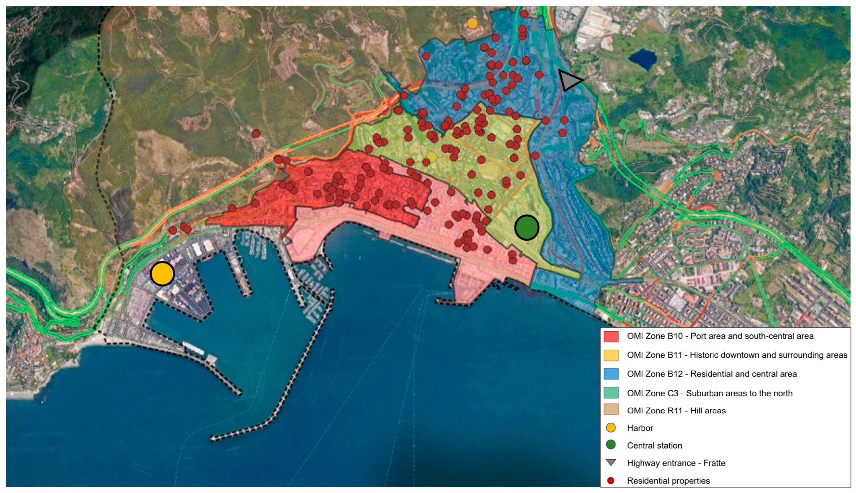
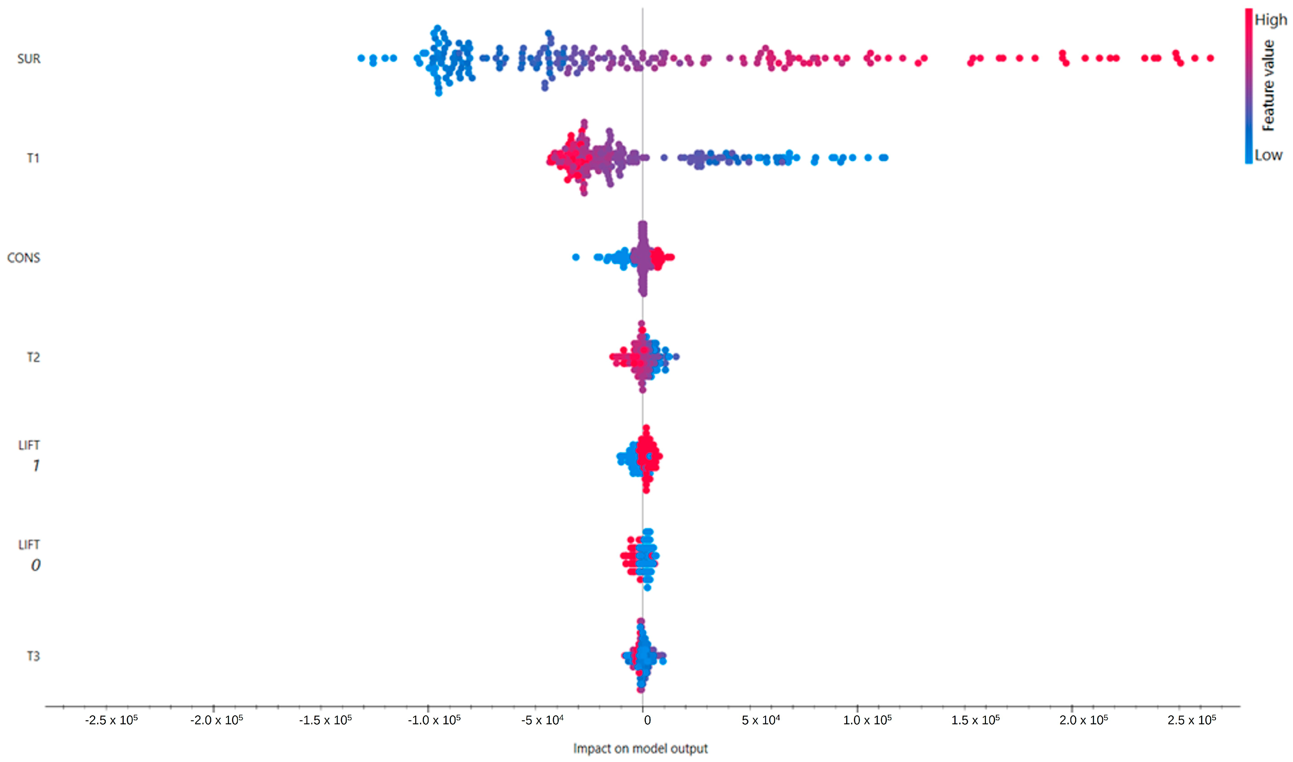
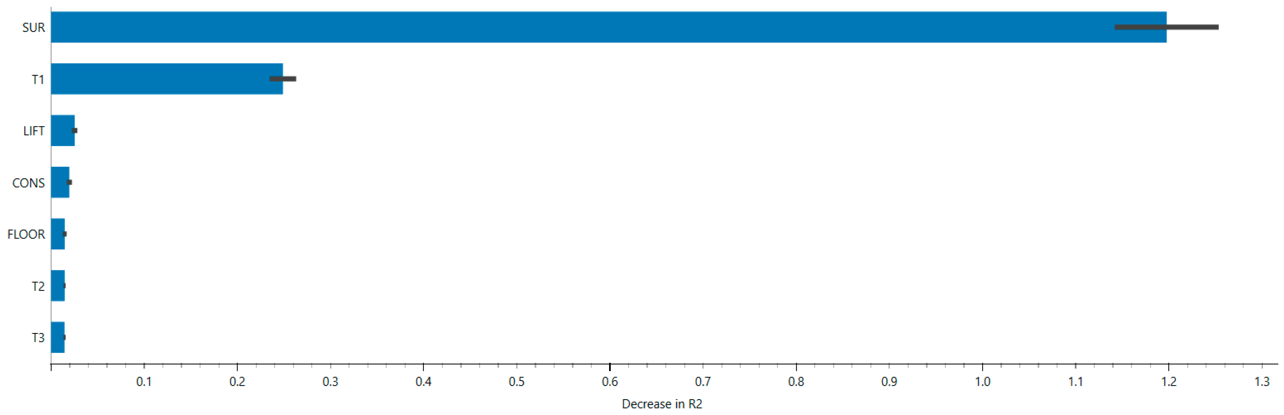
Disclaimer/Publisher’s Note: The statements, opinions and data contained in all publications are solely those of the individual author(s) and contributor(s) and not of MDPI and/or the editor(s). MDPI and/or the editor(s) disclaim responsibility for any injury to people or property resulting from any ideas, methods, instructions or products referred to in the content. |
© 2025 by the authors. Licensee MDPI, Basel, Switzerland. This article is an open access article distributed under the terms and conditions of the Creative Commons Attribution (CC BY) license (https://creativecommons.org/licenses/by/4.0/).