All articles published by MDPI are made immediately available worldwide under an open access license. No special
permission is required to reuse all or part of the article published by MDPI, including figures and tables. For
articles published under an open access Creative Common CC BY license, any part of the article may be reused without
permission provided that the original article is clearly cited. For more information, please refer to
https://www.mdpi.com/openaccess.
Feature papers represent the most advanced research with significant potential for high impact in the field. A Feature
Paper should be a substantial original Article that involves several techniques or approaches, provides an outlook for
future research directions and describes possible research applications.
Feature papers are submitted upon individual invitation or recommendation by the scientific editors and must receive
positive feedback from the reviewers.
Editor’s Choice articles are based on recommendations by the scientific editors of MDPI journals from around the world.
Editors select a small number of articles recently published in the journal that they believe will be particularly
interesting to readers, or important in the respective research area. The aim is to provide a snapshot of some of the
most exciting work published in the various research areas of the journal.
Guido Ferilli is Associate Professor of Economics and Director of the Cultural Industries and at in [...]
Guido Ferilli is Associate Professor of Economics and Director of the Cultural Industries and Complexity Observatory at IULM University in Milan. His research focuses on economics, data science, and European programmes. He conducts international research and consultancy activities in the fields of cultural economics, policy design, and local development. He has extensive experience in coordinating research and policy design projects worldwide.
The TWC Sigma model, part of the Topological Weighted Centroid (TWC) family, is introduced as a spatial framework for source localization in systems where network information is incomplete or unavailable. Its architecture relies on two alternative approaches: one based on nonlinear correlation, capable of capturing complex spatial dependencies among observed signals, and another based on supervised neural networks, which use adaptive learning on a discretized spatial grid to estimate the probability of hidden source localization. In both cases, TWC Sigma provides a robust and consistent mechanism to estimate the probable positions of hidden sources using only spatial coordinates and signal intensity. Applications on both synthetic and real-world datasets—such as those collected by Minna-no Data Site on post-Fukushima radiocesium contamination—confirm the model’s ability to identify both primary and secondary emission zones with strong spatial coherence. These results highlight TWC Sigma as an efficient and interpretable model that can be used both independently and as a complementary tool to more complex network-based frameworks, offering rapid and reliable localization even in the presence of sparse, noisy, or heterogeneous data.
The precise identification of the source of an epidemic, environmental contamination, or propagation phenomenon in complex systems represents a major challenge, where timely and accurate source detection is essential for effective intervention and containment strategies. The accurate and timely identification of the source, commonly referred to as “source detection,” plays a pivotal role in elucidating the underlying propagation mechanisms. Furthermore, it is essential for the proper design of effective containment strategies that also optimize the allocation of the available resources. However, this problem is complicated by several practical and theoretical obstacles: observable data are often partial and noisy, contact networks may be highly complex, dynamic, or completely unknown, and the available information may cover only a fraction of the involved nodes.
The recent literature has proposed a variety of approaches to source localization, each with specific strengths and limitations depending on the scenario. Network-based models are among the most widely studied: the Active Querying Approach dramatically reduces the number of necessary observations using active querying strategies and Bayesian inference, making it well-suited for large and complex networks, but it requires a detailed knowledge of the network structure, which is often unavailable in real-world settings [1]. The PESL algorithm enables source localization in very large networks, exploiting sparse observers and maximum likelihood estimation; it is robust to incomplete and noisy data, but again depends heavily on network topology information [2]. In dynamic networks, where connections between nodes evolve over time, dedicated models can incorporate the temporal sequence of interactions, providing accurate estimates even with partial data, but at the cost of increased computational complexity and the need to trace dynamic connections [3].
Advanced machine learning methods further enrich this landscape. Bayesian generative frameworks with neural networks can probabilistically reconstruct infection trajectories and infer source positions, effectively managing data and parameter uncertainty, but require suitable training and an accurate representation of the underlying network [4]. Graph Neural Networks (GNNs) have shown great power in directly inferring sources from observed data, even in complex and incomplete networks, but are limited by the need for high-quality training data and, at times, by the limited interpretability of results [5]. Topological Data Analysis (TDA) offers a complementary perspective, enabling the description of the global morphology of propagation, identifying clusters and emergent patterns without directly pinpointing the source; its use remains more analytical than predictive [6,7]. Systematic reviews in the field have highlighted the diversity of available approaches—from centrality-based to probabilistic and deep learning methods—emphasizing that the choice of technique should be guided by the nature of the data and the knowledge of the observed system [8].
Despite the sophistication and effectiveness of these approaches, there are still many application contexts where the contact network structure is unknown, inaccessible, or not relevant—as in scenarios dominated by physical distance, spatial geometry, or propagation in open environments. In such cases, many network-based models become difficult to apply or risk introducing unjustified assumptions. To address these needs, the TWC Sigma model is proposed as an alternative framework for source localization in contexts where spatial configuration is the dominant factor. Based solely on spatial data—coordinates of observed points and, when available, signal intensity—TWC Sigma employs correlation algorithms and supervised neural networks to estimate the probability of source localization, discretizing space into a grid and assigning each cell a probability score.
Designed to operate independently of the application domain—be it epidemiological, environmental, or geophysical—TWC Sigma provides a general methodology adaptable to heterogeneous datasets and diverse propagation phenomena. The model’s architecture and validation on real-world data further demonstrate its practical robustness and its capacity to extract meaningful insights even in the absence of detailed structural information.
2. Materials and Methods
2.1. The Topological Weighted Centroid
The approach proposed in this paper, TWC Sigma, belongs to the Topological Weighted Centroid (TWC) family [9], specifically developed for the analysis of bidimensional point distributions. Within this framework, each point may optionally include additional attributes that complement its spatial coordinates (see Equations (1) and (2)).
where
;
;
;
.
where
;
;
.
TWC Sigma is designed to analyze scenarios in which each point, in addition to its spatial position, incorporates an additional variable V that quantifies the intensity of the signal received from a source located at an unknown position within the same domain (see Equation (2)).
where
;
;
;
;
;
.
In the proposed approach, the estimation of unknown source locations is achieved by analyzing the coordinates of observed points and the strength of the signal they receive. Since in a bidimensional space the power of a signal decays as a function of the distance between sender and receiver, when only one source is active, detecting its position using the locations of the observed points is relatively straightforward. However, as the number of unknown sources increases, the problem becomes increasingly complex, requiring advanced methods capable of resolving multiple overlapping propagation patterns.
2.2. The Algorithm
To estimate the proximity of each grid point () to one or more hidden sources, the nonlinear correlation approach adopted by TWC Sigma is articulated in two main steps.
The first step, Nonlinear Transformation, reorganizes the spatial and signal data to reveal complex, nonlinear dependencies between distance and the received signal strength.
The second step, Grid Point Activation, applies analytical or neural computation methods to evaluate, for each grid point, a numerical activation value that expresses its likelihood of being close to a hidden source.
Together, these two steps transform the original spatial distribution of observations into a probabilistic activation map, where high values indicate areas with the highest estimated source influence.
2.2.1. Step a: Nonlinear Transformation
In this phase, the method performs a nonlinear transformation of the distances between each grid point () and all the observed points (), each associated with a signal value .
For each grid point, the Euclidean distances between and all are computed and then ranked, producing the ordered sequence , which represents the spatial arrangement of the observed points relative to .
In parallel, the signal strength values are reordered according to the same ranking, generating a corresponding sequence .
This dual transformation establishes a nonlinear correspondence between distance and signal power, describing how each grid point “perceives” the distribution of signals in its surroundings.
An inverse transformation can also be applied by sorting the signal strengths and reordering the distances accordingly, resulting in and , to obtain a complementary representation based on signal intensity.
Overall, this step constructs a transformed dataset that captures the nonlinear relationships between the spatial structure and signal strength, enabling the identification of complex propagation patterns that cannot be detected by simple linear correlations.
2.2.2. Step b1: Grid Point Activation—Analytical Methods
The purpose of the Grid Point Activation step is to assign each grid point () an activation value, representing the probability or intensity of its proximity to one or more unknown sources.
This step can be implemented using analytical methods—such as the Linear Correlation (LC) and Prior Probability Algorithm (PPA)—which correlate the nonlinear functions derived in Step a (, , , and ) as expressed in Equations (4)–(6).
Linear Correlation:
Master Equation:
Prior Probability Algorithm:
2.2.3. Step b2: Grid Point Activation—ANN
Alternatively, the same process can be carried out using Artificial Neural Networks (ANNs), which generalize and extend the activation computation. In this case, the data generated in Step a are reorganized into a structure suitable for supervised learning: spatial coordinates and signal intensity values serve as inputs, while the target corresponds to the estimated proximity to the hidden source.
During the training phase, the ANN learns the nonlinear relationships among distance, position, and signal strength. In the inference phase, it autonomously computes the activation value for each grid point, effectively replacing the classical correlation equations. This adaptive and flexible approach enables the identification of complex propagation patterns and allows the network to distinguish multiple overlapping source areas with higher precision.
The data points described in the previous section can be reformulated in a format specifically suited for training a supervised Artificial Neural Network (ANN). In particular, the structure of the assigned data, previously illustrated in Equation (3), can be reorganized as follows:
The resulting data structure, as shown in Equation (8), is now appropriate for supervised ANN training.
where
;
;
.
To minimize the loss function during training, we experimented with and compared several types of ANNs: a traditional Multilayer Perceptron (MLP), a Supervised Contractive Map (SVCm), and a BiModal ANN (BM).
The SVCm network employed the following architecture: four input units and one output unit (as specified in Equation (8)), two hidden layers with 24 units each, a learning coefficient (LCoef) of 0.01, and weights initialized within the range . The Multilayer Perceptron (MLP) used the same architecture () with a learning rate of 0.01 and standard sigmoid activation. Each ANN was trained with more than 12 million patterns per epoch.
Additionally, we implemented a novel network topology, the BiModal ANN (BM). In this configuration, the output target is defined by both the intensity of the first input point and its spatial coordinates in a two-dimensional space.
Equation (10) presents how the data structure is adapted for training with this new ANN topology.
where
;
.
After training, the recall (or inference) phase of an ANN exhibits distinctive characteristics. Specifically, the activation value for each grid point is determined through N recall operations, where N is the number of assigned points, according to the following schema.
= the input combination between the k-th coordinates of the grid point and the first of the assigned points, and the output of the k-th grid point.
For each grid point, its activation is computed as either the average or the maximum output value across all possible input combinations. For example, if the mapped area consists of grid points (arranged in 600 rows and 600 columns), and there are assigned points, the recall phase requires 50 evaluations per grid point, resulting in a total of recall operations to process the entire map.
2.2.4. Analytical Foundation of ANN-Based Source Inference
This section provides an analytical explanation of why the ANN architectures used in the TWC Sigma framework are able to infer hidden signal sources from spatial observations and why the recall phase produces highly precise spatial localization. The explanation relies on the mathematical structure of the signal field, the ranking-based feature transformation applied during preprocessing, and the computational structure of the recall phase.
Consider a spatial observation set composed of N measurement points associated with signal intensities . Assume that the signal field is generated by M hidden sources with strength .
Under very general physical conditions, the received intensity can be approximated by a power law attenuation model:
where is the attenuation exponent and represents measurement noise. This equation defines a nonlinear mapping between the hidden source coordinates and observed signals. Although the mapping is not analytically invertible, it preserves a strong topological property: the signal intensity decreases monotonically with distance from each source.
For the special case of a single dominant source S, the signal field becomes . Let be a candidate grid point; if approaches the real source location (), then the distances and therefore . This implies the following:
In other words, the ordering of the distances from the candidate source becomes consistent with the inverse ordering of signal intensities. The preprocessing stage used in the TWC Sigma framework exploits exactly this property. For each candidate grid point , the distances to all the observation points are computed and sorted. The signal intensities are then rearranged according to the same ranking, converting the spatial field into a ranked vector representation . When coincides with a real source, the pair exhibits a highly structured relationship that is absent for most other grid locations. This structure becomes a stable signature that neural networks can learn.
In the presence of multiple sources, the monotonic ordering is partially broken because different observations may be dominated by different sources. However, the ranking patterns still contain piecewise monotonic structures corresponding to the domains of influence of each source. The ANN learns to recognize these nonlinear patterns, approximating a function where represents the likelihood that the candidate location corresponds to a hidden source.
The BM (BiModal) architecture introduces an additional stabilization mechanism. In each training pattern, one input point is used as a pivot reference whose coordinates and intensity are embedded in the target representation. This effectively expresses the spatial configuration in relative coordinates (, ), removing global translation ambiguity and forcing the network to learn relationships that depend only on the internal geometry of the signal field.
2.2.5. Theoretical Analysis: Limitations of Alternative Methods and Advantages of Ranking-Based Representations
This section analyzes alternative computational systems that could theoretically be used to infer hidden signal sources from spatial observations and explains analytically why their performance is generally more limited than the ANN architectures used in the TWC Sigma framework.
Linear regression, correlation models, kernel density estimators, Gaussian processes, and optimization-based inverse models all attempt to reconstruct the signal field through global functional approximations. However, when multiple hidden sources are present, the signal becomes a nonlinear superposition of attenuation functions (Equation (13)), which breaks the global monotonic relationships between signal intensity and distance from any single point.
Theorem 1
(Failure of Global Monotonic Estimators).For a signal field generated by two or more sources with attenuation law , no estimator based on a single global monotonic relation between intensity and distance can uniquely recover all source coordinates.
Proof.
Consider two sources and . For observation points located closer to , the signal is dominated by , while for points closer to the signal is dominated by . The resulting ordering of intensities changes across space. Therefore, no single monotonic function exists such that for any global S. Global estimators thus collapse toward compromise solutions such as centroids or extended maxima. □
Theorem 2
(Consistency of Ranking-Based Nonlinear Estimators).Let the signal field be generated by attenuation functions of the form with bounded noise. Then the ranked representation preserves sufficient topological information to distinguish candidate points near true sources from points far from sources.
Proof.
As approaches a source , the distance vector converges to the true source distances. Because the attenuation function is monotonic in distance, the ranking of intensities becomes increasingly aligned with the ranking of inverse distances. This alignment generates a stable pattern in . Nonlinear estimators such as neural networks can learn to recognize this pattern. As the number of observation points N increases, the ranking structure becomes more stable and the estimator converges toward the true source location. □
Theorem 3
(Multi-Source Separability via MAX Aggregation in Recall).Assume a multi-source field and a recall procedure that, for each candidate grid point , constructs multiple feature vectors by choosing different pivot points p in the observation set, and then aggregates ANN outputs via MAX pooling: . Under mild conditions (bounded noise; each source has a non-empty domain of influence producing pivots whose ranked signatures are dominated by that source), exhibits distinct local maxima in neighborhoods of each true source , enabling the separability of multiple sources even when global rank monotonicity is violated.
Proof.
For each source , define the subset of pivots consisting of observation points whose received signal is dominated (in relative contribution) by source m. For any pivot , the ranked feature construction is locally (for near ) close to the single-source signature induced by ; hence, it matches the patterns seen during training for that source. Therefore is high for in a neighborhood of and low away from it. Taking the maximum over pivots selects, for each , the pivot yields the strongest source-consistent explanation. Consequently, for each m there exists a neighborhood around where is dominated by pivots in and forms a local maximum near . In contrast, mean aggregation averages across incompatible pivots from different sources, producing smoother maps and potentially merging peaks. Thus MAX aggregation acts as a mixture-of-experts selector that preserves multiple sharp maxima corresponding to distinct hidden sources. □
Practical implication. MAX aggregation behaves as a deterministic latent assignment (hard gating) mechanism, akin to max pooling in deep networks, selecting the pivot/source-consistent “expert” for each grid location. This is precisely why recall can separate multiple sources while global estimators (LC/PP) collapse toward compromise solutions.
2.2.6. Computational Complexity and Parallel Recall
For a grid containing G candidate pixels and N observations, computing ranked distances requires approximately operations per pixel. The ANN forward pass requires operations, where W is the number of network weights.
The total sequential recall complexity is therefore as follows:
A crucial property of the algorithm is that each candidate location is evaluated independently of all the other locations—there are no dependencies between evaluations. This means the recall stage can be fully parallelized. If processing units are available (CPU cores, GPU threads, or distributed nodes), the candidate grid can be partitioned into subsets, each evaluated independently:
In GPU implementations, thousands of candidate pixels can be evaluated simultaneously because all forward passes use identical network weights but different input vectors. This architecture therefore scales almost linearly with the number of available processing units. The independence of pixel evaluations makes the algorithm particularly suitable for massively parallel hardware such as modern GPU architectures, facilitating the reconstruction of high-resolution maps of hidden signal sources without prohibitive computational cost.
2.2.7. The Experiments
In this study, two complementary types of experiments were conducted: synthetic data experiments and real-world data experiments. The synthetic benchmarks comprise five experiments grouped into three progressively complex levels: two single-source configurations, two two-source configurations, and one three-source configuration, which differ in terms of the number of hidden signal sources and the density of the observation points (Table A1, Table A2, Table A3, Table A4, Table A5, Table A6, Table A7, Table A8 and Table A9; Figure A1, Figure A2, Figure A3, Figure A4, Figure A5, Figure A6, Figure A7, Figure A8 and Figure A9). These controlled scenarios allow us to evaluate the behaviour and scalability of the algorithms as the spatial configuration becomes increasingly challenging, without providing detailed descriptions of each individual setup.
In parallel, a second set of experiments was carried out using real environmental radiation data from the Minna-no Data Site (MDS) project [10]. This dataset, collected across eastern Japan after the Fukushima Daiichi accident, enables us to test the TWC Sigma framework under realistic conditions, where measurement noise, irregular sampling, and heterogeneous spatial patterns naturally occur.
2.2.8. Synthetic Data Generation
We designed a series of experiments using synthetic data to evaluate the accuracy of the algorithms described earlier. Our approach was as follows. First, we generated a set of random points distributed across a two-dimensional plane (referred to as assigned points). To generate the data, the following formula was employed:
where noise = 0.01.
The activation value () of each point () is determined with respect to a set of n sources (, or emitters). A small noise parameter () is introduced to ensure numerical stability and to avoid degenerate solutions. Distances are then normalized by scaling them with respect to the maximum separation observed between points and sources. This normalization provides a consistent reference framework for the computation of activation values, reducing the influence of local spatial irregularities and enabling robust comparisons across the entire point distribution.
Next, we randomly placed one or more hidden sources emitting a signal, and calculated the strength of this signal at each assigned point using the equation presented in (20).
where
;
;
;
;
.
Quality Measure
Finally, we introduce a quality measure, denoted as Q, to evaluate the clustering performance. For each probability band, we consider both the associated probability and the relative spatial coverage in terms of pixels, defined as
where is the probability assigned to band b and is its percentage area. The higher the overlap of sources with bands of elevated probability and spatial quality, the more effective the resulting spatial mapping can be considered.
Real-World Data: Fukushima Radiocesium Dispersion
To extend the evaluation of the TWC Sigma framework beyond controlled synthetic environments, we applied the model to a large real-world dataset describing the spatial distribution of radiocesium contamination following the Fukushima Daiichi nuclear accident.
On 11 March 2011, the Great East Japan Earthquake in the Tohoku region triggered an offshore earthquake, followed by a tsunami and the damage to the Fukushima Daiichi Nuclear Power Plant (FDNPP). As a consequence of this, large quantities of radionuclides, including cesium isotopes, were released into the environment, dispersing across both the land and sea. In the immediate aftermath of the disaster, official assessments relied almost exclusively on aerial monitoring surveys to estimate air dose rates, while ground-based soil sampling remained limited primarily to Fukushima Prefecture. As a result, the contamination status of many regions—particularly in the Kanto area—remained largely uncertain during the early post-accident phase. To fill this gap and to provide a more accurate and transparent understanding of radioactive contamination, citizen-led initiatives, such as Minna-no Data Site (“Everyone’s Data Site”), were established [10,11].
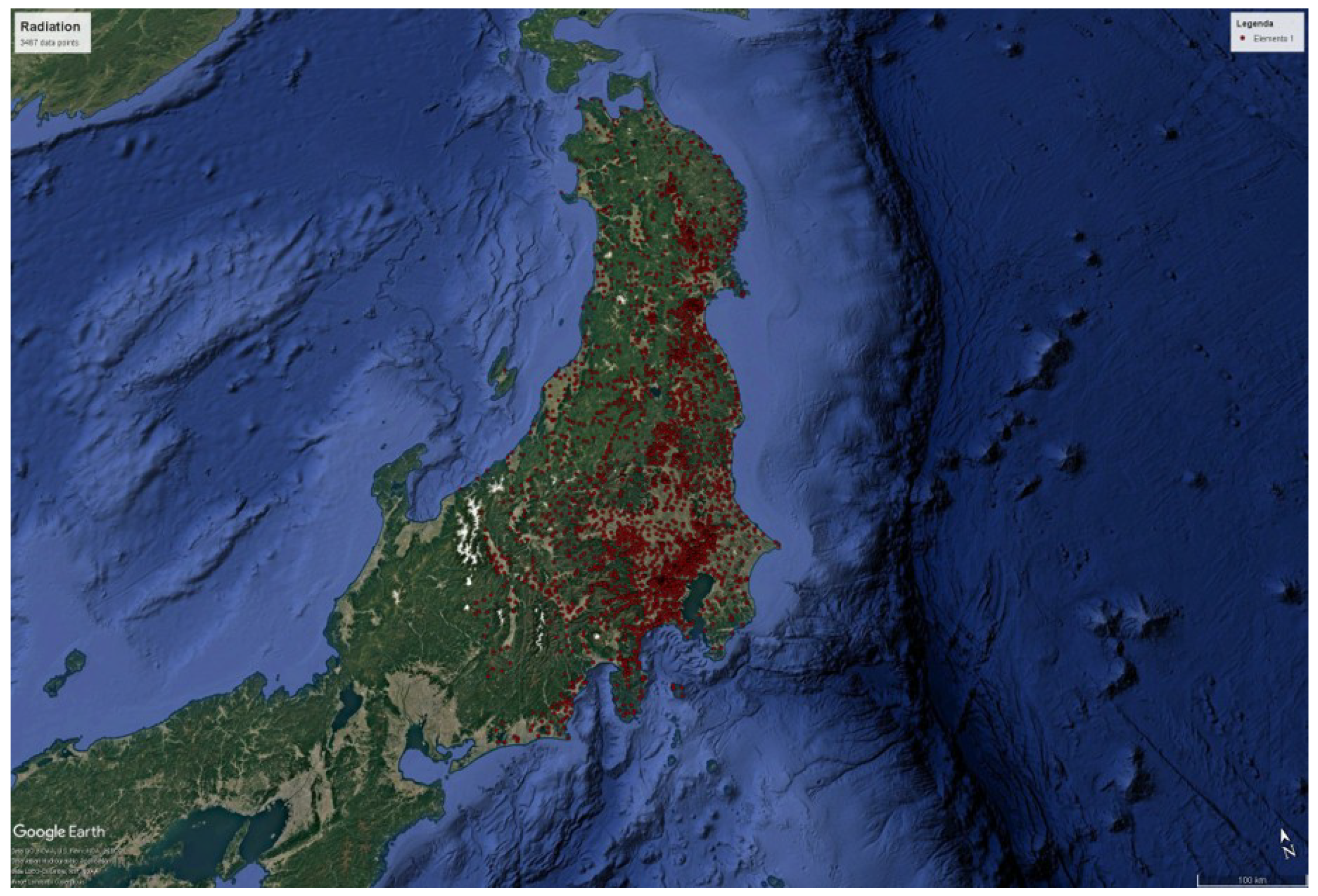
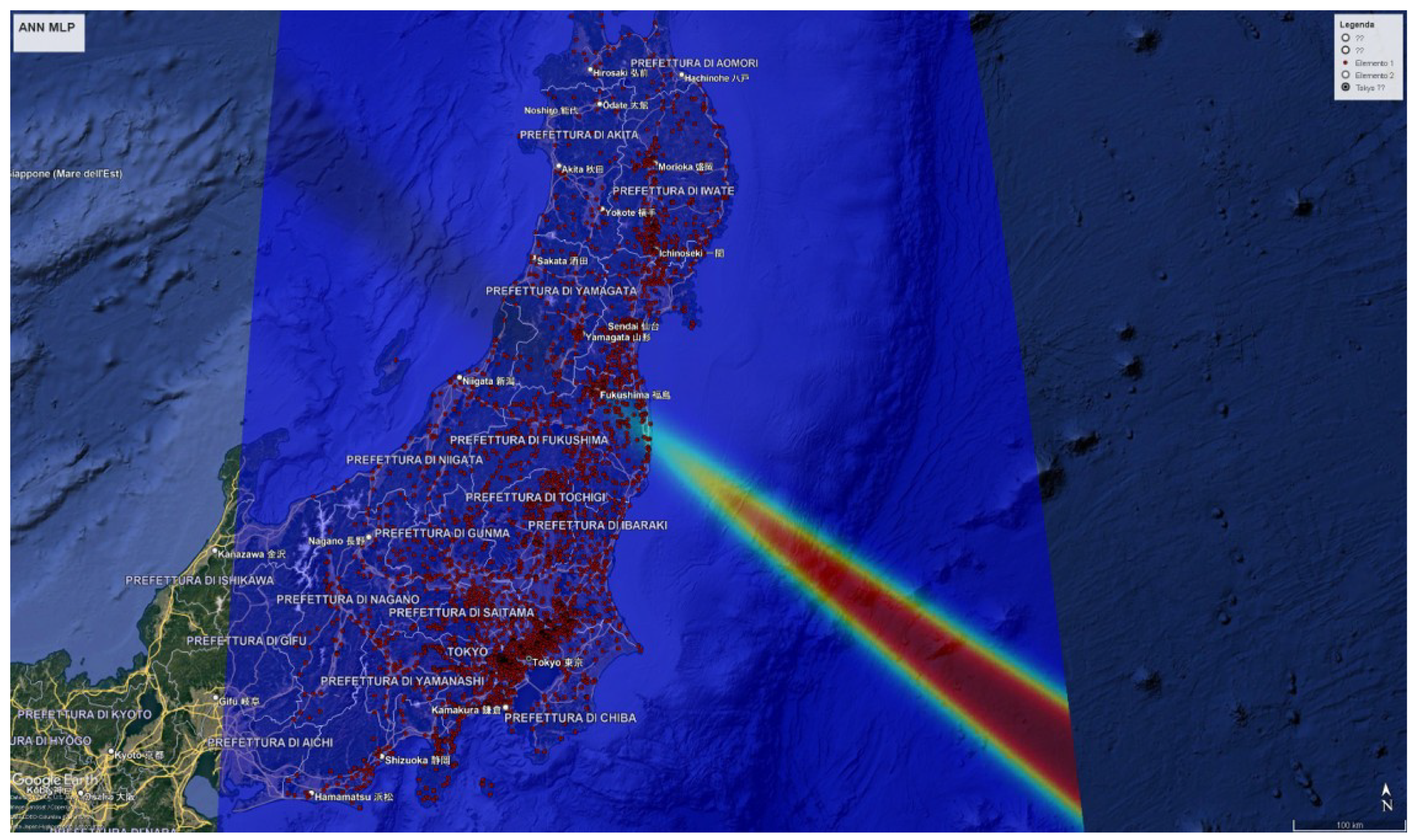
The Minna-no Data Site (MDS) project launched a standardized and large-scale soil sampling campaign covering 17 prefectures of eastern Japan officially designated by the government as radiation-contaminated regions. Between 2014 and 2017, over 30 citizen laboratories collaborated to collect and analyze more than 3000 soil samples under a unified protocol (Figure 1). The sampling sites were selected in non-decontaminated and unplowed areas to best reflect the conditions close to the accident period. Surface soil (0–5 cm depth) was collected, avoiding artificial hotspots such as gutters or drainage areas, and georeferenced via GPS. When possible, air dose rates were measured at both 50 cm and 1 m above ground. The use of NaI scintillation counters and Ge semiconductor detectors—each annually calibrated with standard radioactive sources—ensured consistent measurements expressed in Bq/kg (dry weight). Cross-validation among laboratories and correction methods were implemented to mitigate detector-specific biases and interferences from natural radionuclides such as those of uranium and thorium series.
In this experiment, the dataset collected by the Minna-no Data Site (MDS) project was processed to evaluate the applicability of the TWC Sigma framework to real post-accident environmental data. The MDS dataset, comprising 3467 records, includes precise geographical coordinates for each sampling location and the corresponding quantitative measurements of radioactive cesium concentration in soil, expressed as the total deposition of (Bq/m2). These two variables—the spatial coordinates and the total cesium concentration—were used as the sole inputs for the elaboration. The experiment aimed to reconstruct the probable diffusion patterns and identify the most likely emission sources across the north-central part of Honshu Island, Japan’s largest island.
3. Results
3.1. Synthetic Data Experiments
Across all experimental configurations, the TWC Sigma framework was evaluated using two families of algorithms—nonlinear correlation methods (Linear Correlation, LC; Prior Probability, PP) and supervised Artificial Neural Networks (Multilayer Perceptron, MLP; Supervised Contractive Map, SVCm). The performance was assessed by comparing the scalar probability fields generated by each method against the true location of one or more hidden sources.
3.1.1. Single-Source Scenarios
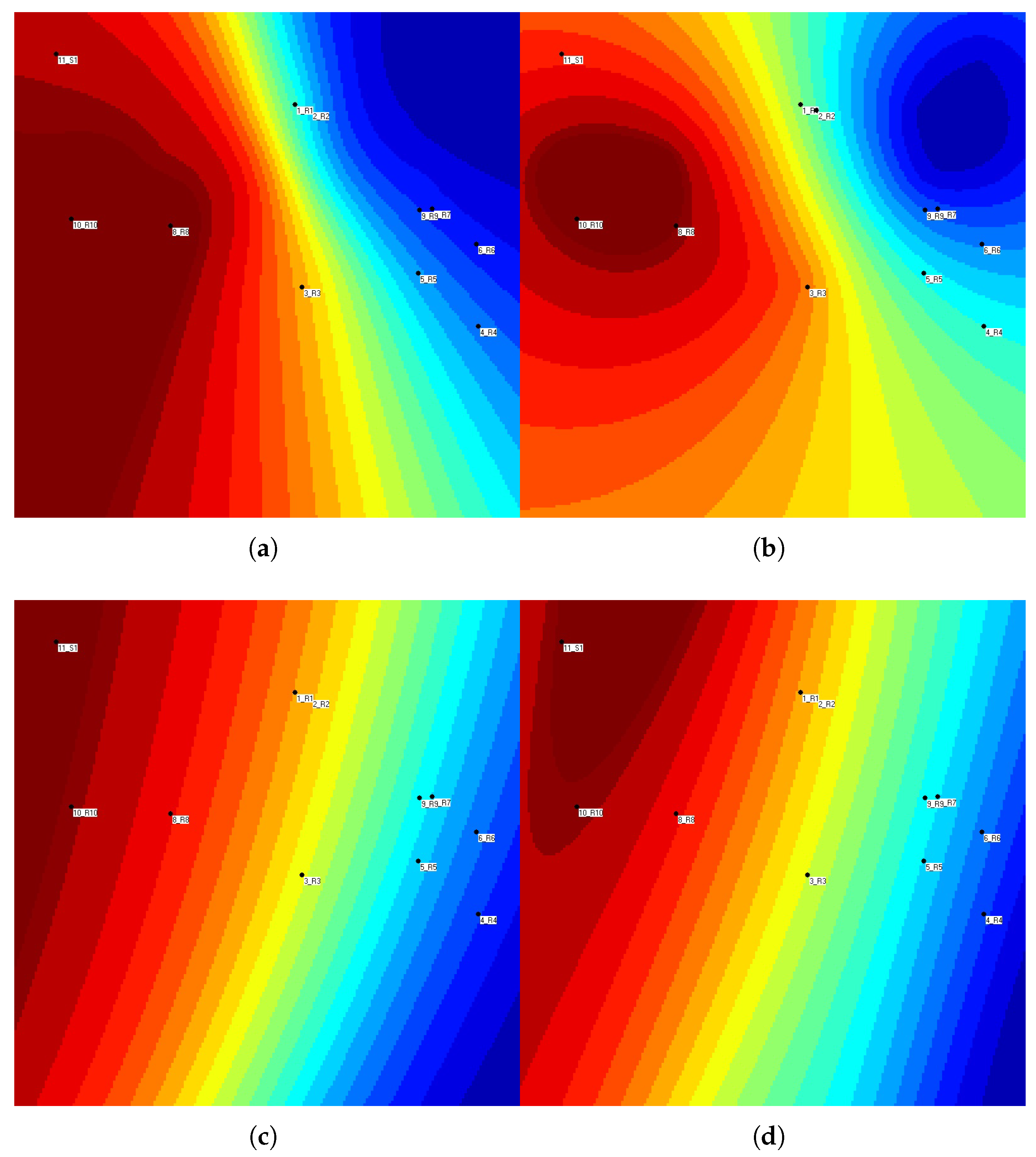
Two initial experiments (Experiment #1 and #2) were designed to assess the performance under minimal complexity, with only one hidden emitter. In both cases—the source outside the convex hull (Exp. #1) and source embedded within it (Exp. #2)—all the algorithms successfully identified the correct emission zone, producing robust and spatially coherent activation maxima.
In Experiment #1 (Figure A2; Table A2), where the source lay outside the observation area, neural models achieved slightly higher precision scores than correlation approaches (e.g., MLP and SVCm vs. LC ; PP ).
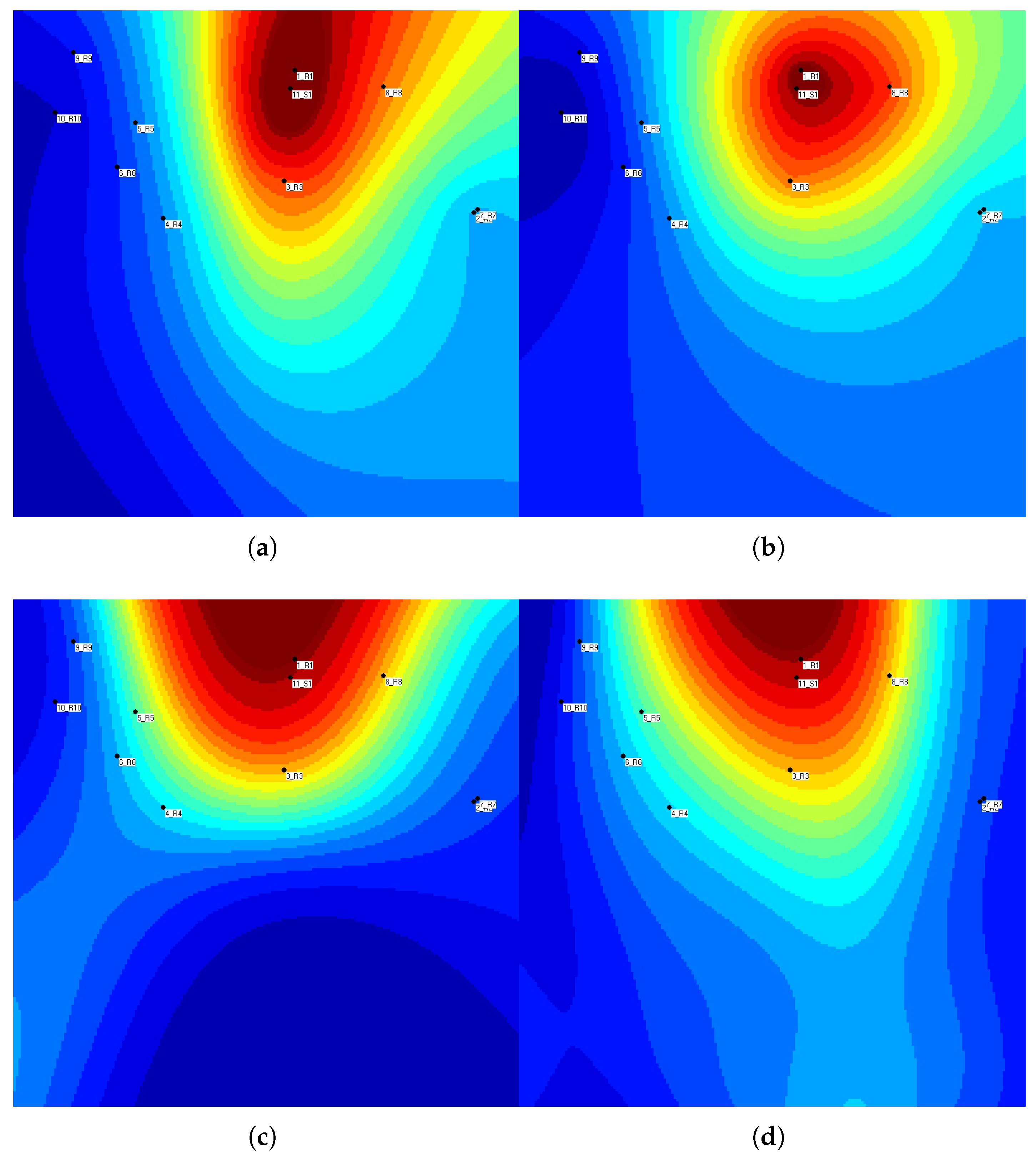
In Experiment #2 (Figure A4; Table A4), the configuration was again well resolved by all methods, although correlation-based algorithms slightly outperformed neural networks (LC ; PP vs. MLP/SVCm ).
Overall, these analyses confirm that when the spatial signal is generated by a single source, TWC Sigma yields stable and consistent results regardless of the algorithmic strategy.
3.1.2. Two-Source Configurations
Increasing the number of hidden sources produced marked differences between the correlation-based and ANN-based methods.
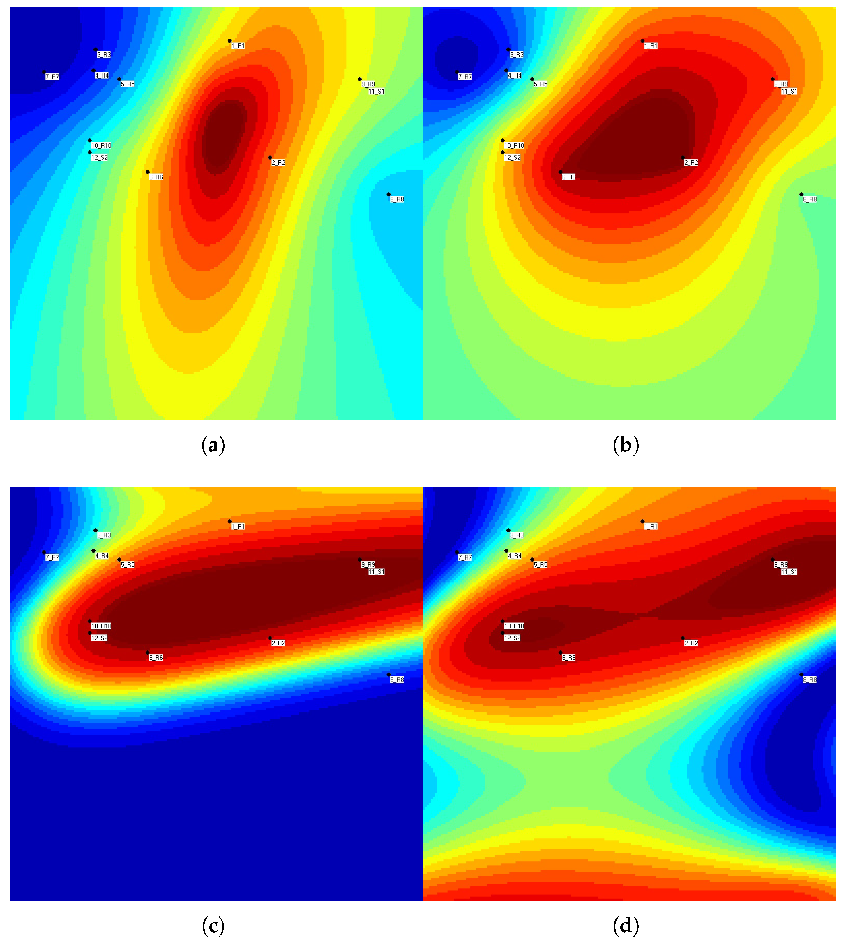
In Experiment #3 (ten receivers and two sources; Figure A6 and Table A6), both LC and PP converged toward an averaged “intermediate” location, failing to resolve the two true emission zones (LC precision window: –; PP: –). By contrast, all the ANN models detected two distinct maxima, with the SVCm and BM networks producing the most localized and symmetric clusters (MLP ; SVCm ).
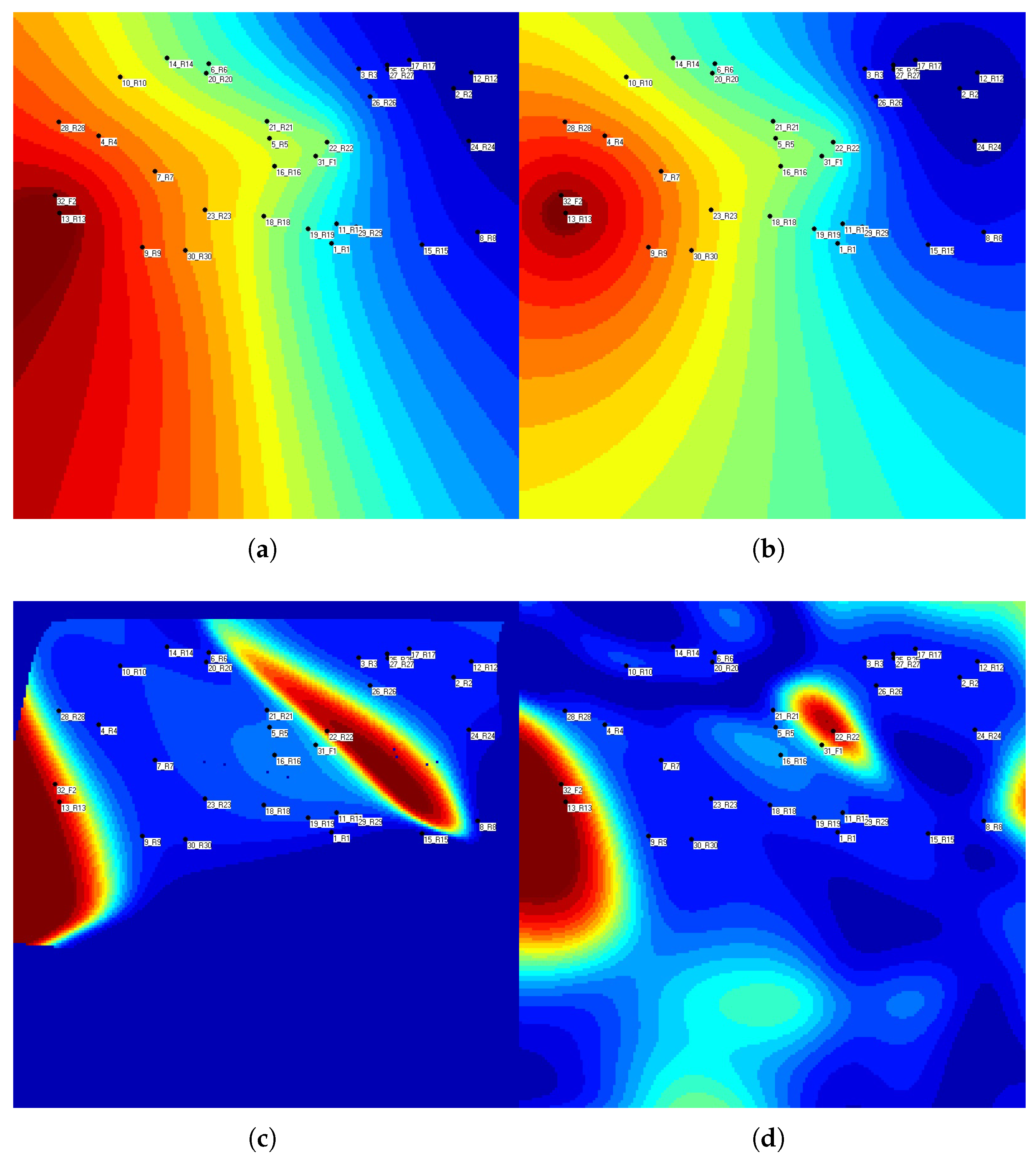
Experiment #4 (thirty receivers and two sources; Figure A8 and Table A8) reproduced these findings in a denser spatial scenario. Correlation algorithms identified only one of the two sources and systematically collapsed probability mass toward the leftmost region of the map. Neural networks correctly isolated both sources: the MLP generated broader hot areas, while SVCm models provided sharply delineated, source-specific peaks with very high precision (SVCm –).
3.1.3. Three-Source Configuration
The most complex synthetic scenario (Experiment #5: forty receivers and three emitters; Figure A10 and Table A10) further amplified performance gaps.
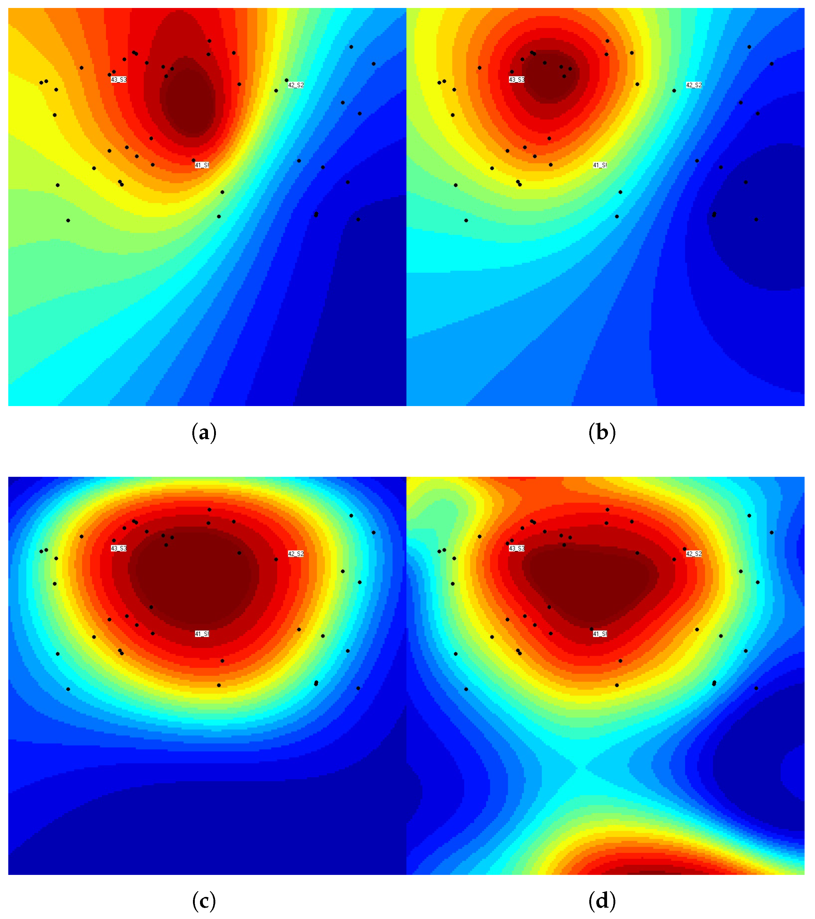
LC and PP located either a single barycentric “virtual” source or only one true emitter. MLP and SVCm networks identified a broad region covering all three real sources, although the SVCm models occasionally produced a secondary false positive cluster in the southern area. Quantitatively, neural networks demonstrated substantially higher precision (MLP –; SVCm –) than correlation-based methods (LC –; PP –).
3.1.4. Overall Trends in Synthetic Data Experiments
Taken together, the synthetic experiments reveal a clear and consistent pattern. When only one source is present, all the algorithms perform reliably, producing stable activation maps and correctly identifying the emission zone with only minor differences in precision. However, as soon as multiple sources are introduced, the behavior of the methods diverges sharply. Correlation-based algorithms tend to merge the effects of different emitters into a single averaged hotspot, losing the ability to distinguish separate sources. In contrast, neural network models—especially the SVCm and BM—maintain distinct activation peaks and accurately resolve each source even in complex or overlapping configurations. Overall, neural approaches scale far better with increasing spatial complexity, whereas correlation methods remain effective primarily in simpler, single-source scenarios.
3.2. Real-World Data Experiments
The dataset contains several thousand ground-based measurements of total cesium deposition recorded across the northern–central region of Honshu. The spatial distribution of these observations is highly heterogeneous, reflecting both the uneven population density of the surveyed areas and the practical constraints of field sampling (Figure 1).
Unlike the synthetic scenarios, where the number, position, and relative intensities of the emission sources are known a priori, the Fukushima dataset represents a complex and environmentally mediated diffusion process influenced by multiple physical mechanisms. Atmospheric dispersion, turbulent transport, precipitation-driven washout, topography, and post-depositional hydrological redistribution all contribute to the observed spatial variability. This makes source localization considerably more challenging and provides a stringent test for the robustness of TWC Sigma.
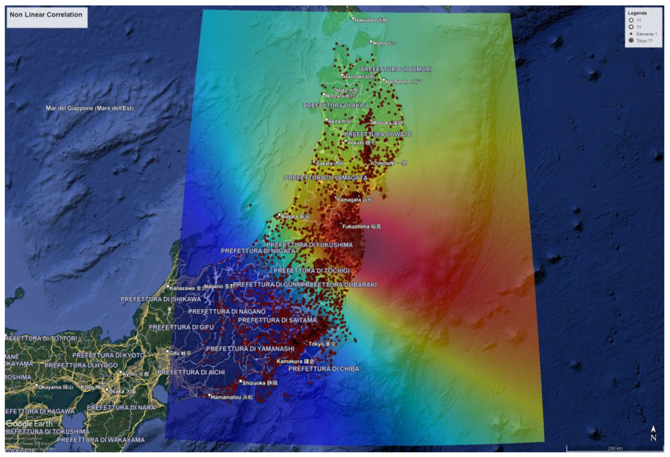
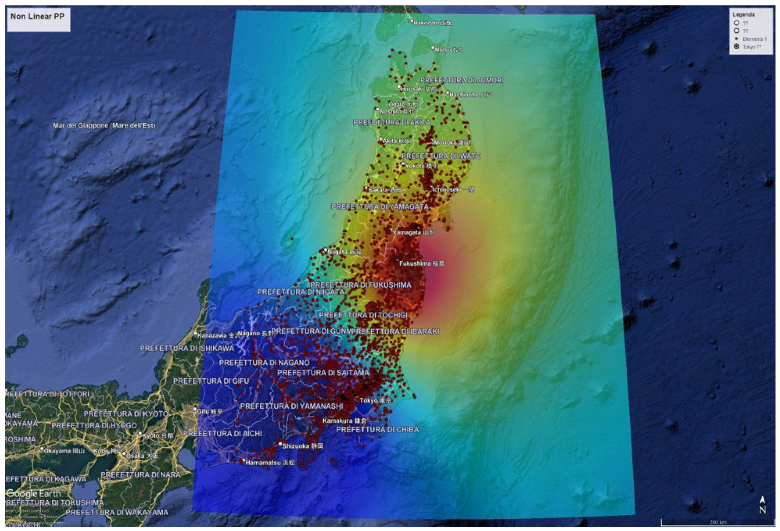
Despite these complexities, all algorithmic variants consistently identified the Fukushima coastline—coincident with the reactor complex—as the region of highest activation probability (Figure 2 and Figure 3). Both correlation-based methods (LC and PP) generated smooth and coherent activation fields, each forming a broad hotspot tightly concentrated around the primary release area. These results align with the well-established understanding that the majority of initial cesium deposition originated directly from atmospheric releases during the early phases of the accident.
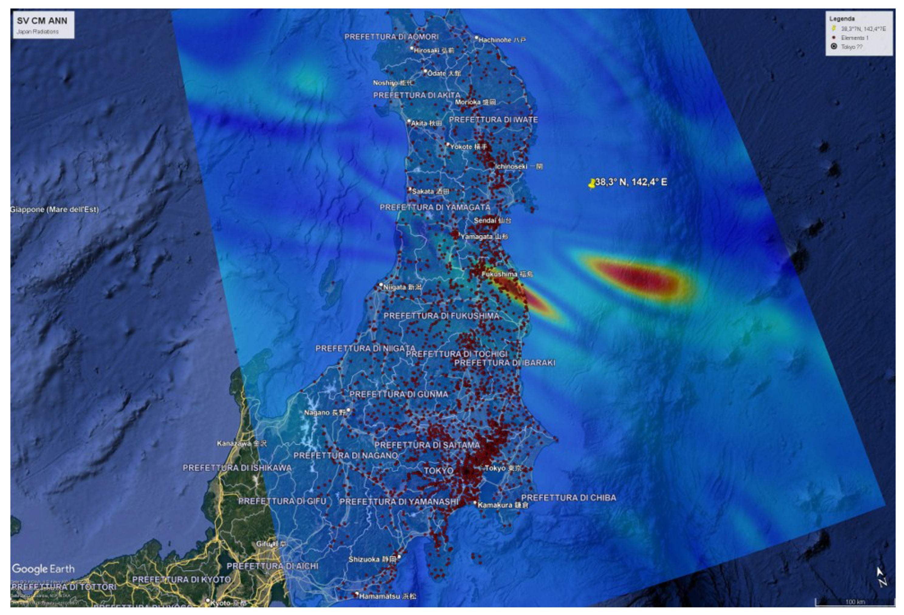
Neural models delivered a more articulated and nuanced representation of the underlying spatial morphology. The MLP and SVCm networks, in addition to resolving the primary coastal hotspot, revealed a secondary activation ridge extending eastward over the marine area (Figure 4 and Figure 5). The morphology of this secondary structure is consistent with hydrodynamic processes that may have redistributed part of the radionuclide load through coastal currents in the months following the accident.
Although this structure does not reflect a secondary emission source, it is consistent with known hydrodynamic processes that redistributed part of the radionuclide load through coastal currents in the months following the accident [12,13,14]. The capacity of the neural variants to detect such secondary spatial gradients suggests that TWC Sigma, when combined with ANN-based inference, can capture not only source proximity but also downstream environmental signatures embedded within the spatial data.
4. Discussion
The experimental evidence, obtained from both synthetic and real-world datasets, demonstrates that TWC Sigma is capable of delivering reliable and consistent results even when data are limited or incomplete. This property is especially valuable when compared with other advanced source localization approaches, which often depend on the availability of rich structural or temporal data.
For instance, Active Querying strategies have been designed to minimize the number of required observations by leveraging active search and Bayesian inference; however, their applicability in practice is limited, as they require a complete and detailed knowledge of the underlying network structure—an assumption that frequently does not hold in real-world cases where network data is incomplete or unavailable [1]. Similarly, the PESL algorithm, although robust to noise and partial observations, still fundamentally relies on having access to the topological information of the contact network, and is therefore often unfeasible in scenarios lacking such data [2].
Models specifically developed for dynamic networks provide the ability to reconstruct the temporal sequence of interactions, thus improving localization performance in evolving contexts. Nevertheless, these methods rapidly become computationally demanding and require detailed temporal datasets, which are rarely available at the required granularity in operational contexts [3].
Probabilistic and generative methods based on neural networks, such as Bayesian frameworks, have been shown to effectively handle uncertainty and to probabilistically infer source positions within a network. However, the effectiveness of these models is closely tied to the accuracy and completeness of both the data and the network representation used during training [4].
TWC Sigma overcomes these barriers by relying solely on spatial coordinates (and optionally signal strength), without the need for any knowledge of the underlying network or large, high-quality training sets. This makes TWC Sigma especially advantageous in public health or environmental scenarios where only sparse or irregular data is available.
In contrast, advanced deep learning solutions like Graph Neural Networks (GNNs) require large, well-annotated datasets for training, and even when sufficient data is present, they may function as “black boxes,” making the interpretation of their results less accessible to practitioners [5]. Topological Data Analysis (TDA) methods provide valuable insights into the overall structure and clustering of the propagation process, but do not directly pinpoint the origin of the spreading event, thus offering analytical rather than predictive value in source localization [7].
Moreover, more traditional approaches—including centrality, probabilistic, or general deep learning models—are often highly sensitive to missing or low-quality data, with their reliability and precision quickly deteriorating when the dataset is incomplete or noisy [8].
5. Conclusions
The results suggest that the TWC Sigma model may represent a promising approach for source localization in contexts dominated by spatial dynamics and characterized by incomplete or heterogeneous data. The model exhibits good computational efficiency and can serve as a complementary tool to more complex methods, particularly in cases where information about contact networks is unavailable or of limited relevance.
The application of the proposed method to real-world data, such as the Minna-no Data Site dataset, highlights its potential as an effective analytical framework for complex spatial phenomena. In this context, the model not only enables the rapid identification of potential origin areas of propagation, but also reveals subtle and non-trivial spatial structures that are often difficult to detect with conventional approaches. This capability is particularly relevant in scenarios where direct measurements or detailed network information is limited or unavailable, as it allows analysts to infer meaningful spatial dynamics from minimal data while maintaining computational efficiency.
Regarding future developments, extending the model to dynamic data (such as a time series of observations) would be necessary to more accurately represent real-world phenomena in which sources vary over time or interact with each other. Furthermore, integrating heterogeneous data sources (such as sociodemographic, clinical, or environmental information) would improve the model’s predictive capabilities and practical usefulness, providing support for both the early identification of sources and the planning of interventions. These directions respond to the growing need for tools capable of adapting to complex and variable scenarios, supporting more informed and effective decisions in health, environmental, and other contexts.
Author Contributions
Conceptualization, P.M.B.; methodology, P.M.B., M.B., R.P. and G.M.; software P.M.B. and G.M.; validation, P.M.B. and G.M.; formal analysis, P.M.B.; investigation, P.M.B., M.B., R.P. and G.M.; resources, G.F., P.M.B. and G.M.; data curation, P.M.B., G.M., G.F., M.B. and R.P.; writing—original draft preparation, P.M.B., G.M., M.B. and R.P.; writing—review and editing, P.M.B., M.B., R.P. and G.F.; visualization, P.M.B., G.M., M.B. and R.P.; supervision, P.M.B., G.M., M.B. and R.P.; project administration, P.M.B., M.B. and R.P.; and funding, P.M.B. All authors have read and agreed to the published version of the manuscript.
Funding
This research received no external funding.
Data Availability Statement
This study uses two types of data. The synthetic datasets were generated by the authors for benchmarking purposes and are fully reproducible from the procedures described in the manuscript. The real-world dataset used for the Fukushima case study was provided by Minna-no Data Site (MDS) under a confidentiality agreement for research purposes only. This dataset may not be redistributed by the authors. Requests for access to the MDS data should be directed to the data provider (https://en.minnanods.net).
Acknowledgments
The authors thank Minna-no Data Site for providing the dataset used in this study. These data were used solely for research purposes under the terms defined by the data provider. The usual disclaimer applies.
Conflicts of Interest
The authors declare no conflicts of interest.
Abbreviations
The following abbreviations are used in this manuscript:
ANN
Artificial Neural Network
BM
BiModal Neural Network
LC
Linear Correlation
MLP
Multilayer Perceptron
MDS
Minna-no Data Site
PPA
Prior Probability Algorithm
PP
Prior Probability (used in text as shorthand for PPA)
Precis.
Precision
Q
Quality Measure
SVCm
Supervised Contractive Map
TDA
Topological Data Analysis
TWC
Topological Weighted Centroid
TWC Sigma
Topological Weighted Centroid Sigma Model
Vi
Received Signal Strength at point i
Pk
k-th Grid Point (in discretized spatial domain)
Pi
i-th Assigned Point (receiver)
MaxD
Maximum Distance in the Map
Appendix A
Appendix A.1. Experiments with One Hidden Source
Appendix A.1.1. Experiment 1—Source Located Separately from the Entities
Figure A1.
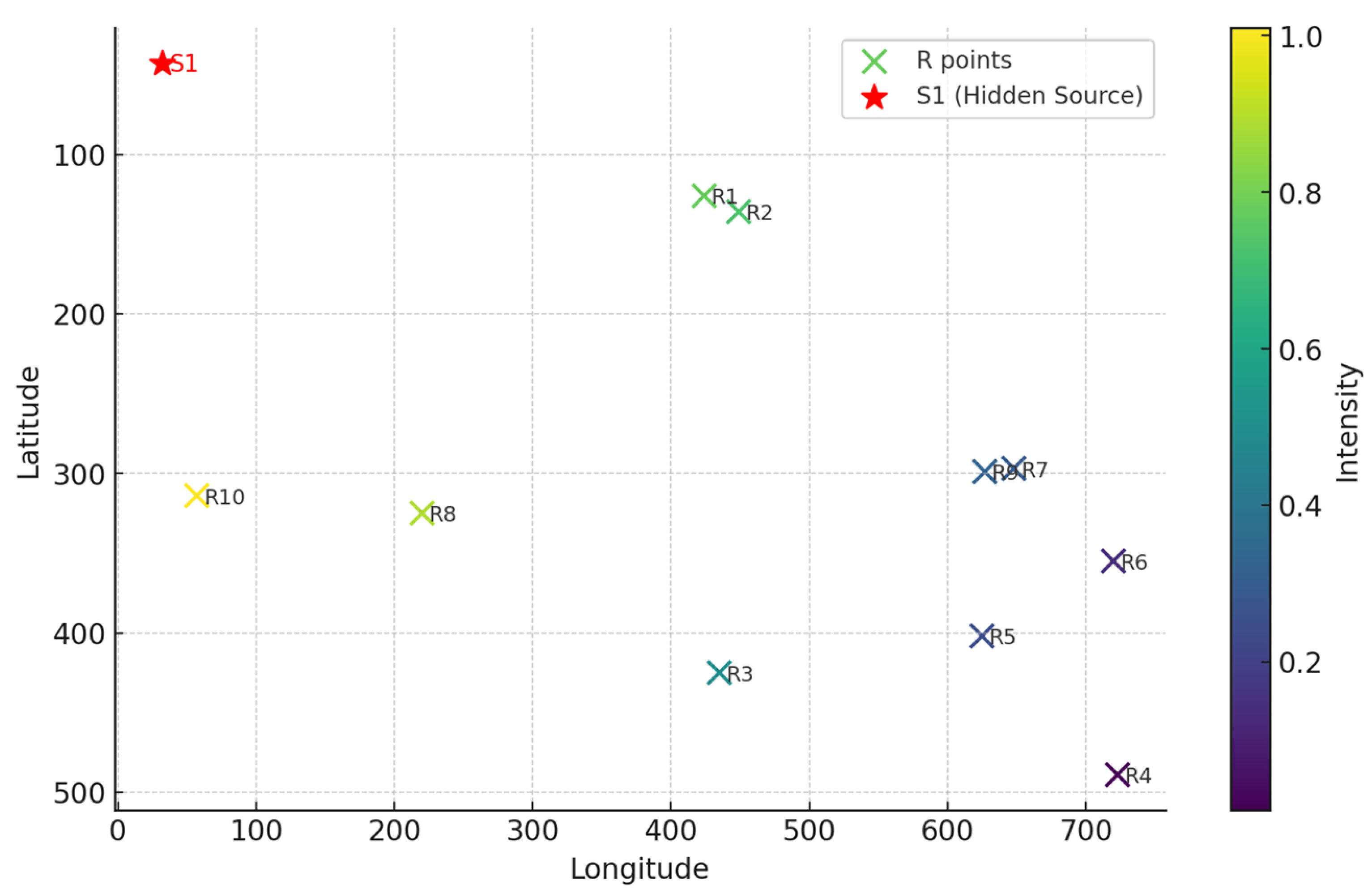
The map representing the data of Table A1. The red color shows the position of the hidden source transmitting the signal.
Figure A1.
The map representing the data of Table A1. The red color shows the position of the hidden source transmitting the signal.
Table A1.
Experiment 1—Position of the points (receivers and source). The last row reports the coordinates of the hidden signal source, which is unknown to the algorithms under evaluation.
Table A1.
Experiment 1—Position of the points (receivers and source). The last row reports the coordinates of the hidden signal source, which is unknown to the algorithms under evaluation.
Type
Entity
Longitude
Latitude
Intensity
Data
R1
424
126
0.7764
Data
R2
449
136
0.7282
Data
R3
435
425
0.4955
Data
R4
723
489
0.0100
Data
R5
625
402
0.2448
Data
R6
720
355
0.1317
Data
R7
648
297
0.2937
Data
R8
220
325
0.8887
Data
R9
627
299
0.3275
Data
R10
57
314
1.0100
Hidden Source
S1
32
43
-
Figure A2.
Experiment 1—Scalar probability field computed by the algorithms. Color gradients in the heat map indicate values from maximum (deep red) to minimum (deep blue). From left to right and from top to bottom: (a) Linear Correlation; (b) Prior Probability; (c) Multilayer Perceptron; and (d) Supervised Contractive Map.
Figure A2.
Experiment 1—Scalar probability field computed by the algorithms. Color gradients in the heat map indicate values from maximum (deep red) to minimum (deep blue). From left to right and from top to bottom: (a) Linear Correlation; (b) Prior Probability; (c) Multilayer Perceptron; and (d) Supervised Contractive Map.
Table A2.
Quality measures for Experiment 1. The table shows, for each algorithm, the probability range in which the source is located (in bold), the fraction of area covered by the probability zone, and the corresponding quality score (corresponding to the bold entries).
Table A2.
Quality measures for Experiment 1. The table shows, for each algorithm, the probability range in which the source is located (in bold), the fraction of area covered by the probability zone, and the corresponding quality score (corresponding to the bold entries).
Bin Min
Bin Max
Mean
LC Extent
LC Precis.
PProb Extent
PProb Precis.
MLP Extent
MLP Precis.
SVCm Extent
SVCm Precis.
0.00
0.05
0.025
0.08050
0.02299
0.03735
0.02407
0.01988
0.02450
0.02035
0.02449
0.05
0.10
0.075
0.04110
0.07192
0.03290
0.07253
0.02710
0.07297
0.02060
0.07346
0.10
0.15
0.125
0.03443
0.12070
0.02855
0.12143
0.03280
0.12090
0.02463
0.12192
0.15
0.20
0.175
0.03008
0.16974
0.02180
0.17119
0.03745
0.16845
0.03045
0.16967
0.20
0.25
0.225
0.02900
0.21848
0.02165
0.22013
0.04270
0.21539
0.03875
0.21628
0.25
0.30
0.275
0.03028
0.26667
0.02295
0.26869
0.04563
0.26245
0.04580
0.26241
0.30
0.35
0.325
0.03295
0.31429
0.02553
0.31670
0.04300
0.31103
0.04720
0.30966
0.35
0.40
0.375
0.03150
0.36319
0.02938
0.36398
0.04125
0.35953
0.04873
0.35673
0.40
0.45
0.425
0.02883
0.41275
0.03625
0.40959
0.04033
0.40786
0.04955
0.40394
0.45
0.50
0.475
0.02750
0.46194
0.05108
0.45074
0.04023
0.45589
0.04858
0.45193
0.50
0.55
0.525
0.02670
0.51098
0.05530
0.49597
0.04070
0.50363
0.04725
0.50019
0.55
0.60
0.575
0.02708
0.55943
0.04958
0.54649
0.04190
0.55091
0.04620
0.54844
0.60
0.65
0.625
0.02818
0.60739
0.04963
0.59398
0.04395
0.59753
0.04610
0.59619
0.65
0.70
0.675
0.03010
0.65468
0.05413
0.63847
0.04715
0.64317
0.04675
0.64344
0.70
0.75
0.725
0.03265
0.70133
0.07363
0.67162
0.05163
0.68757
0.04860
0.68977
0.75
0.80
0.775
0.03660
0.74664
0.10558
0.69318
0.05845
0.72970
0.05253
0.73429
0.80
0.85
0.825
0.04278
0.78971
0.09198
0.74912
0.06868
0.76834
0.05985
0.77562
0.85
0.90
0.875
0.05943
0.82300
0.07868
0.80616
0.08553
0.80017
0.07803
0.80673
0.90
0.95
0.925
0.11555
0.81812
0.07263
0.85782
0.10920
0.82399
0.12125
0.81284
0.95
1.00
0.975
0.23980
0.74120
0.06648
0.91019
0.08748
0.88971
0.08383
0.89327
Appendix A.1.2. Experiment 2—Source Located Between the Entities
Figure A3.
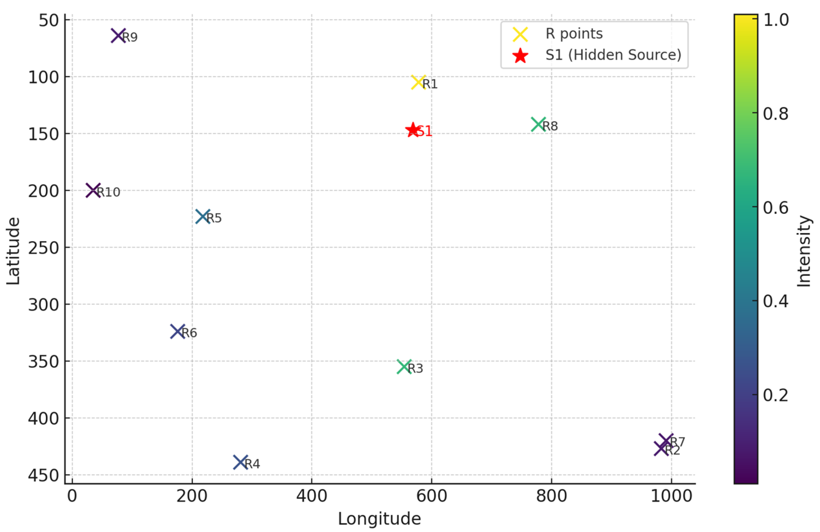
The map representing the data of Table A3. The red color shows the position of the hidden source transmitting the signal.
Figure A3.
The map representing the data of Table A3. The red color shows the position of the hidden source transmitting the signal.
Figure A4.
Experiment 2—Scalar probability field computed by the algorithms. Color gradients in the heat map indicate values from maximum (deep red) to minimum (deep blue). From left to right and from top to bottom: (a) Linear Correlation; (b) Prior Probability; (c) Multilayer Perceptron; and (d) Supervised Contractive Map.
Figure A4.
Experiment 2—Scalar probability field computed by the algorithms. Color gradients in the heat map indicate values from maximum (deep red) to minimum (deep blue). From left to right and from top to bottom: (a) Linear Correlation; (b) Prior Probability; (c) Multilayer Perceptron; and (d) Supervised Contractive Map.
Table A3.
Experiment 2—Position of the points (receivers and source). The last row reports the coordinates of the hidden signal source, which is unknown to the algorithms under evaluation.
Table A3.
Experiment 2—Position of the points (receivers and source). The last row reports the coordinates of the hidden signal source, which is unknown to the algorithms under evaluation.
Type
Entity
Longitude
Latitude
Intensity
Data
R1
578
105
1.0100
Data
R2
983
427
0.0811
Data
R3
554
355
0.6743
Data
R4
281
439
0.2663
Data
R5
218
223
0.3704
Data
R6
176
324
0.2243
Data
R7
991
420
0.0754
Data
R8
778
142
0.6711
Data
R9
77
64
0.0865
Data
R10
35
200
0.0100
Hidden Source
S1
568
147
-
Table A4.
Quality measures for Experiment 2. The table shows, for each algorithm, the probability range in which the source is located (in bold), the fraction of area covered by the probability zone, and the corresponding quality score (corresponding to the bold entries).
Table A4.
Quality measures for Experiment 2. The table shows, for each algorithm, the probability range in which the source is located (in bold), the fraction of area covered by the probability zone, and the corresponding quality score (corresponding to the bold entries).
Bin Min
Bin Max
Mean
LC Extent
LC Precis.
PProb Extent
PProb Precis.
MLP Extent
MLP Precis.
SVCm Extent
SVCm Precis.
0.00
0.05
0.025
0.04278
0.02393
0.07703
0.02307
0.23000
0.01925
0.02473
0.02438
0.05
0.10
0.075
0.06223
0.07033
0.11423
0.06643
0.11075
0.06669
0.08163
0.06888
0.10
0.15
0.125
0.13468
0.10817
0.07390
0.11576
0.10308
0.11212
0.14233
0.10721
0.15
0.20
0.175
0.14768
0.14916
0.06110
0.16431
0.11933
0.15412
0.14883
0.14896
0.20
0.25
0.225
0.16013
0.18897
0.11075
0.20008
0.10773
0.20076
0.14855
0.19158
0.25
0.30
0.275
0.08918
0.25048
0.13830
0.23697
0.04170
0.26353
0.11823
0.24249
0.30
0.35
0.325
0.05120
0.30836
0.06768
0.30301
0.03258
0.31441
0.05058
0.30856
0.35
0.40
0.375
0.04065
0.35976
0.04853
0.35680
0.02640
0.36510
0.03845
0.36058
0.40
0.45
0.425
0.03953
0.40820
0.04000
0.40800
0.02208
0.41562
0.03130
0.41170
0.45
0.50
0.475
0.03775
0.45707
0.03540
0.45819
0.01980
0.46560
0.02683
0.46226
0.50
0.55
0.525
0.03145
0.50849
0.03358
0.50737
0.01798
0.51556
0.02390
0.51245
0.55
0.60
0.575
0.02725
0.55933
0.03133
0.55699
0.01700
0.56523
0.02143
0.56268
0.60
0.65
0.625
0.02410
0.60994
0.02713
0.60805
0.01643
0.61473
0.02025
0.61234
0.65
0.70
0.675
0.02213
0.66007
0.02433
0.65858
0.01595
0.66423
0.01875
0.66234
0.70
0.75
0.725
0.02303
0.70831
0.02225
0.70887
0.01640
0.71311
0.01813
0.71186
0.75
0.80
0.775
0.02163
0.75824
0.01978
0.75967
0.01673
0.76204
0.01780
0.76121
0.80
0.85
0.825
0.01908
0.80926
0.01773
0.81038
0.01810
0.81007
0.01790
0.81023
0.85
0.90
0.875
0.01508
0.86181
0.01713
0.86002
0.02048
0.85708
0.01813
0.85914
0.90
0.95
0.925
0.01073
0.91508
0.01863
0.90777
0.02440
0.90243
0.01900
0.90743
0.95
1.00
0.975
0.00478
0.97034
0.02625
0.94941
0.02815
0.94755
0.01830
0.95716
Appendix A.1.3. Experiment 3—Two Sources with Ten Entities
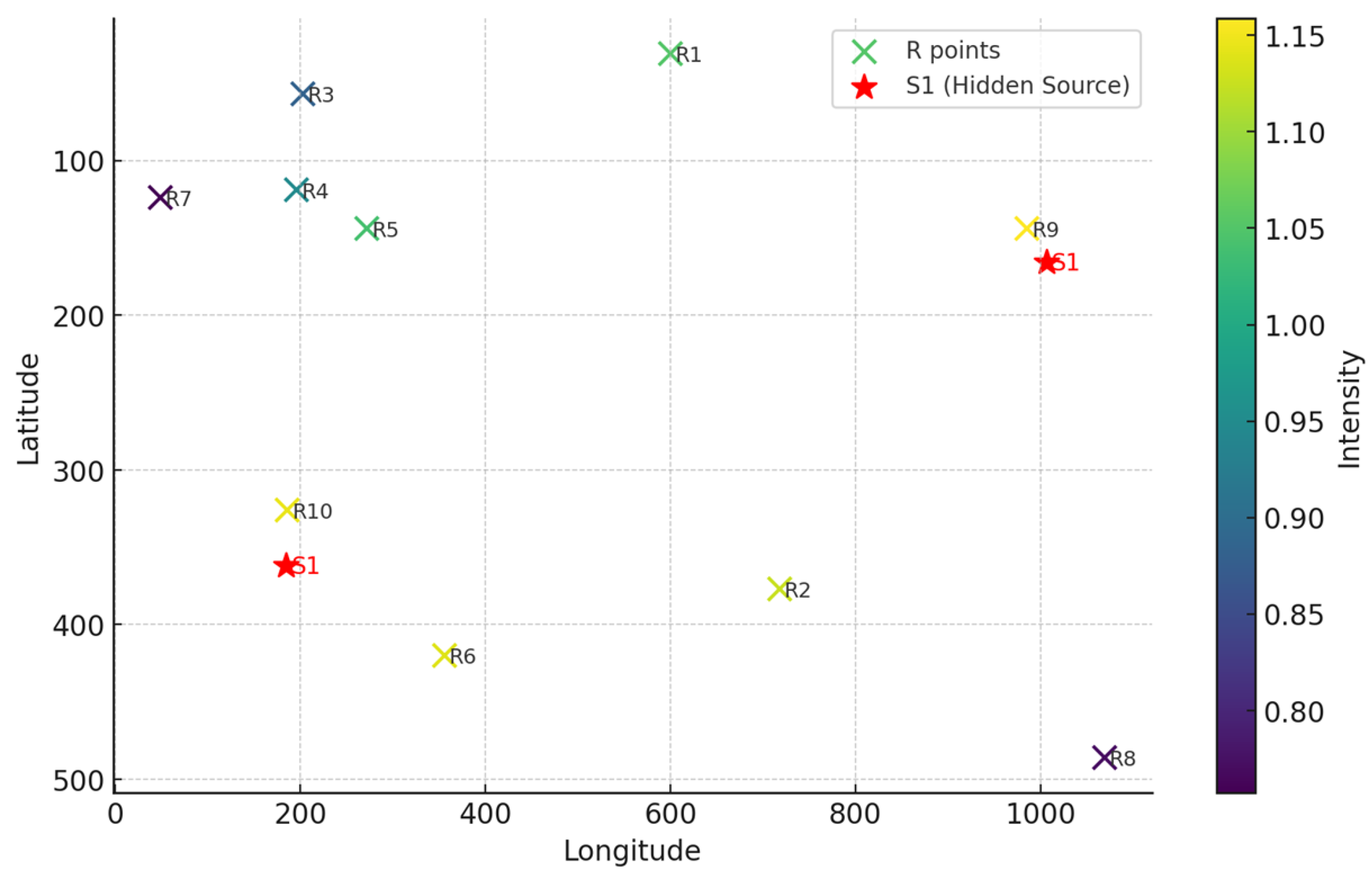
Figure A5.
The map representing the data of Table A5. The red color shows the position of the hidden sources transmitting the signal.
Figure A5.
The map representing the data of Table A5. The red color shows the position of the hidden sources transmitting the signal.
Figure A6.
Experiment 3—Scalar probability field computed by the algorithms. Color gradients in the heat map indicate values from maximum (deep red) to minimum (deep blue). From left to right and from top to bottom: (a) Linear Correlation; (b) Prior Probability; (c) Multilayer Perceptron; and (d) Supervised Contractive Map.
Figure A6.
Experiment 3—Scalar probability field computed by the algorithms. Color gradients in the heat map indicate values from maximum (deep red) to minimum (deep blue). From left to right and from top to bottom: (a) Linear Correlation; (b) Prior Probability; (c) Multilayer Perceptron; and (d) Supervised Contractive Map.
Table A5.
Experiment 3—Position of the points (receivers and sources). The two last rows report the coordinates of the two hidden signal sources, which are unknown to the algorithms under evaluation.
Table A5.
Experiment 3—Position of the points (receivers and sources). The two last rows report the coordinates of the two hidden signal sources, which are unknown to the algorithms under evaluation.
Type
Entity
Longitude
Latitude
Intensity
Data
R1
600
31
1.0520
Data
R2
718
377
1.1258
Data
R3
203
57
0.8825
Data
R4
196
119
0.9485
Data
R5
272
144
1.0408
Data
R6
356
420
1.1385
Data
R7
49
124
0.7572
Data
R8
1069
486
0.7715
Data
R9
985
144
1.1588
Data
R10
186
326
1.1460
Hidden Source
S1
1006
166
-
Hidden Source
S2
185
362
-
Table A6.
Quality measures for Experiment 3. The table shows, for each algorithm, the probability range in which the source is located (in bold), the fraction of area covered by the probability zone, and the corresponding quality score (corresponding to the bold entries).
Table A6.
Quality measures for Experiment 3. The table shows, for each algorithm, the probability range in which the source is located (in bold), the fraction of area covered by the probability zone, and the corresponding quality score (corresponding to the bold entries).
Bin Min
Bin Max
Mean
LC Extent
LC Precis.
PProb Extent
PProb Precis.
MLP Extent
MLP Precis.
SVCm Extent
SVCm Precis.
0.00
0.05
0.025
0.03778
0.02406
0.01525
0.02462
0.44308
0.01392
0.05778
0.02356
0.05
0.10
0.075
0.01695
0.07373
0.02125
0.07341
0.03753
0.07219
0.02900
0.07283
0.10
0.15
0.125
0.01580
0.12303
0.01070
0.12366
0.02470
0.12191
0.02103
0.12237
0.15
0.20
0.175
0.01648
0.17212
0.00863
0.17349
0.01973
0.17155
0.01753
0.17193
0.20
0.25
0.225
0.01875
0.22078
0.00828
0.22314
0.01668
0.22125
0.01763
0.22103
0.25
0.30
0.275
0.03340
0.26582
0.00870
0.27261
0.01570
0.27068
0.01923
0.26971
0.30
0.35
0.325
0.07438
0.30083
0.00968
0.32186
0.01530
0.32003
0.02660
0.31636
0.35
0.40
0.375
0.10965
0.33388
0.01145
0.37071
0.01465
0.36951
0.03465
0.36201
0.40
0.45
0.425
0.09203
0.38589
0.03433
0.41041
0.01428
0.41893
0.04583
0.40552
0.45
0.50
0.475
0.08863
0.43290
0.19428
0.38272
0.01440
0.46816
0.07445
0.43964
0.50
0.55
0.525
0.09415
0.47557
0.14578
0.44847
0.01565
0.51678
0.06110
0.49292
0.55
0.60
0.575
0.10023
0.51737
0.09073
0.52283
0.01693
0.56527
0.05150
0.54539
0.60
0.65
0.625
0.08080
0.57450
0.07533
0.57792
0.02238
0.61102
0.05050
0.59344
0.65
0.70
0.675
0.06653
0.63010
0.06730
0.62957
0.04360
0.64557
0.05480
0.63801
0.70
0.75
0.725
0.04960
0.68904
0.06270
0.67954
0.03020
0.70311
0.06508
0.67782
0.75
0.80
0.775
0.03583
0.74724
0.05663
0.73112
0.02970
0.75198
0.07798
0.71457
0.80
0.85
0.825
0.02680
0.80289
0.05360
0.78078
0.03213
0.79850
0.08068
0.75844
0.85
0.90
0.875
0.02030
0.85724
0.04655
0.83427
0.03840
0.84140
0.06540
0.81778
0.90
0.95
0.925
0.01523
0.91092
0.04155
0.88657
0.05478
0.87433
0.10135
0.83125
0.95
1.00
0.975
0.01173
0.96357
0.04233
0.93373
0.10523
0.87241
0.05293
0.92340
Appendix A.1.4. Experiment 4—Two Sources with 30 Entities
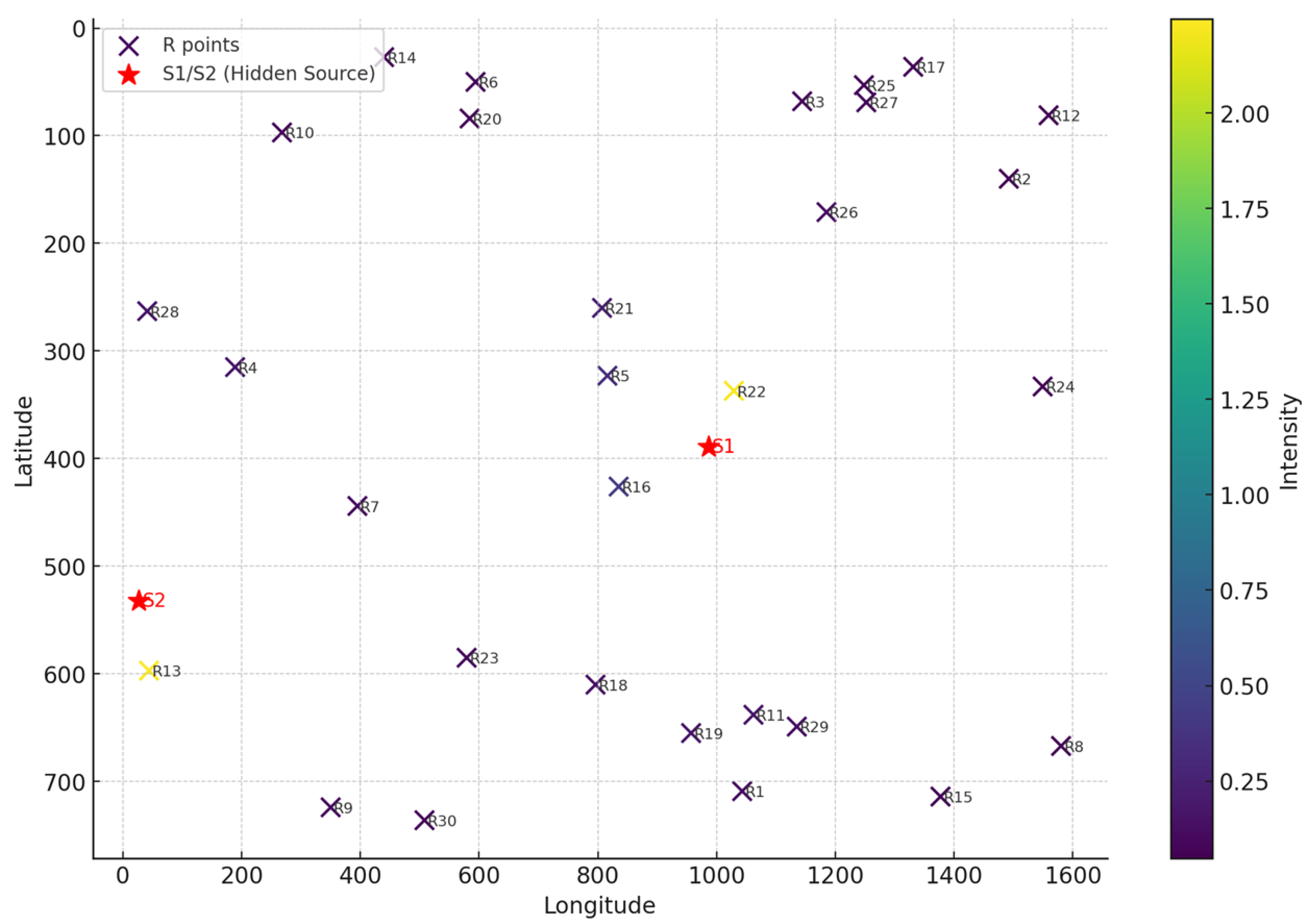
Figure A7.
The map representing the data of Table A7. The red color shows the position of the hidden source transmitting the signal.
Figure A7.
The map representing the data of Table A7. The red color shows the position of the hidden source transmitting the signal.
Table A7.
Experiment 4—Position of the points (receivers and sources). The last two rows report the coordinates of the hidden signal source, which is unknown to the algorithms under evaluation.
Table A7.
Experiment 4—Position of the points (receivers and sources). The last two rows report the coordinates of the hidden signal source, which is unknown to the algorithms under evaluation.
Type
Entity
Longitude
Latitude
Intensity
Data
R1
1043
709
0.1241
Data
R2
1492
140
0.0558
Data
R3
1144
68
0.1050
Data
R4
189
315
0.1720
Data
R5
816
323
0.3357
Data
R6
594
50
0.0753
Data
R7
395
444
0.1182
Data
R8
1580
667
0.0474
Data
R9
350
724
0.1102
Data
R10
268
97
0.0771
Data
R11
1062
638
0.1768
Data
R12
1559
81
0.0476
Data
R13
44
597
2.2461
Data
R14
440
27
0.0668
Data
R15
1377
714
0.0641
Data
R16
835
426
0.4488
Data
R17
1331
36
0.0662
Data
R18
796
610
0.1545
Data
R19
957
655
0.1710
Data
R20
584
84
0.0788
Data
R21
807
260
0.2401
Data
R22
1029
337
2.2260
Data
R23
579
585
0.1015
Data
R24
1549
333
0.0555
Data
R25
1248
53
0.0809
Data
R26
1185
171
0.1416
Data
R27
1252
69
0.0836
Data
R28
41
263
0.1688
Data
R29
1135
649
0.1394
Data
R30
508
736
0.0853
Hidden Source
S1
986
389
-
Hidden Source
S2
27
532
-
Table A8.
Quality measures for Experiment 4. The table shows, for each algorithm, the probability range in which the source is located (in bold), the fraction of area covered by the probability zone, and the corresponding quality score (corresponding to the bold entries).
Table A8.
Quality measures for Experiment 4. The table shows, for each algorithm, the probability range in which the source is located (in bold), the fraction of area covered by the probability zone, and the corresponding quality score (corresponding to the bold entries).
Bin Min
Bin Max
Mean
LC Extent
LC Precis.
PProb Extent
PProb Precis.
MLP Extent
MLP Precis.
SVCm Extent
SVCm Precis.
0.00
0.05
0.025
0.06190
0.02345
0.06235
0.02344
0.53893
0.01153
0.14088
0.02148
0.05
0.10
0.075
0.05298
0.07103
0.04705
0.07147
0.03710
0.07222
0.17008
0.06224
0.10
0.15
0.125
0.05205
0.11849
0.03605
0.12049
0.16293
0.10463
0.25598
0.09300
0.15
0.20
0.175
0.05413
0.16553
0.03763
0.16842
0.07450
0.16196
0.10895
0.15593
0.20
0.25
0.225
0.05595
0.21241
0.04540
0.21479
0.03015
0.21822
0.07033
0.20918
0.25
0.30
0.275
0.04775
0.26187
0.05958
0.25862
0.01393
0.27117
0.05118
0.26093
0.30
0.35
0.325
0.04265
0.31114
0.07793
0.29967
0.01050
0.32159
0.05093
0.30845
0.35
0.40
0.375
0.04055
0.35979
0.06845
0.34933
0.00888
0.37167
0.03865
0.36051
0.40
0.45
0.425
0.04058
0.40776
0.06503
0.39736
0.00795
0.42162
0.01860
0.41710
0.45
0.50
0.475
0.04340
0.45439
0.06803
0.44269
0.00723
0.47157
0.00910
0.47068
0.50
0.55
0.525
0.04630
0.50069
0.07103
0.48771
0.00695
0.52135
0.00720
0.52122
0.55
0.60
0.575
0.04850
0.54711
0.08270
0.52745
0.00600
0.57155
0.00668
0.57116
0.60
0.65
0.625
0.05220
0.59238
0.07905
0.57559
0.00633
0.62105
0.00635
0.62103
0.65
0.70
0.675
0.05630
0.63700
0.05743
0.63624
0.00623
0.67080
0.00620
0.67082
0.70
0.75
0.725
0.05540
0.68484
0.04363
0.69337
0.00658
0.72023
0.00605
0.72061
0.75
0.80
0.775
0.05108
0.73542
0.03418
0.74851
0.00703
0.76956
0.00623
0.77018
0.80
0.85
0.825
0.05103
0.78290
0.02698
0.80275
0.00763
0.81871
0.00650
0.81964
0.85
0.90
0.875
0.05965
0.82281
0.02243
0.85538
0.00943
0.86675
0.00755
0.86839
0.90
0.95
0.925
0.06438
0.86545
0.01518
0.91096
0.01383
0.91221
0.00985
0.91589
0.95
1.00
0.975
0.02825
0.94746
0.00498
0.97015
0.04295
0.93312
0.02775
0.94794
Figure A8.
Experiment 4—Scalar probability field computed by the algorithms. Color gradients in the heat map indicate values from maximum (deep red) to minimum (deep blue). From left to right and from top to bottom: (a) Linear Correlation; (b) Prior Probability; (c) Multilayer Perceptron; and (d) Supervised Contractive Map.
Figure A8.
Experiment 4—Scalar probability field computed by the algorithms. Color gradients in the heat map indicate values from maximum (deep red) to minimum (deep blue). From left to right and from top to bottom: (a) Linear Correlation; (b) Prior Probability; (c) Multilayer Perceptron; and (d) Supervised Contractive Map.
Appendix A.1.5. Experiment 5—Three Sources with 40 Entities
Table A9.
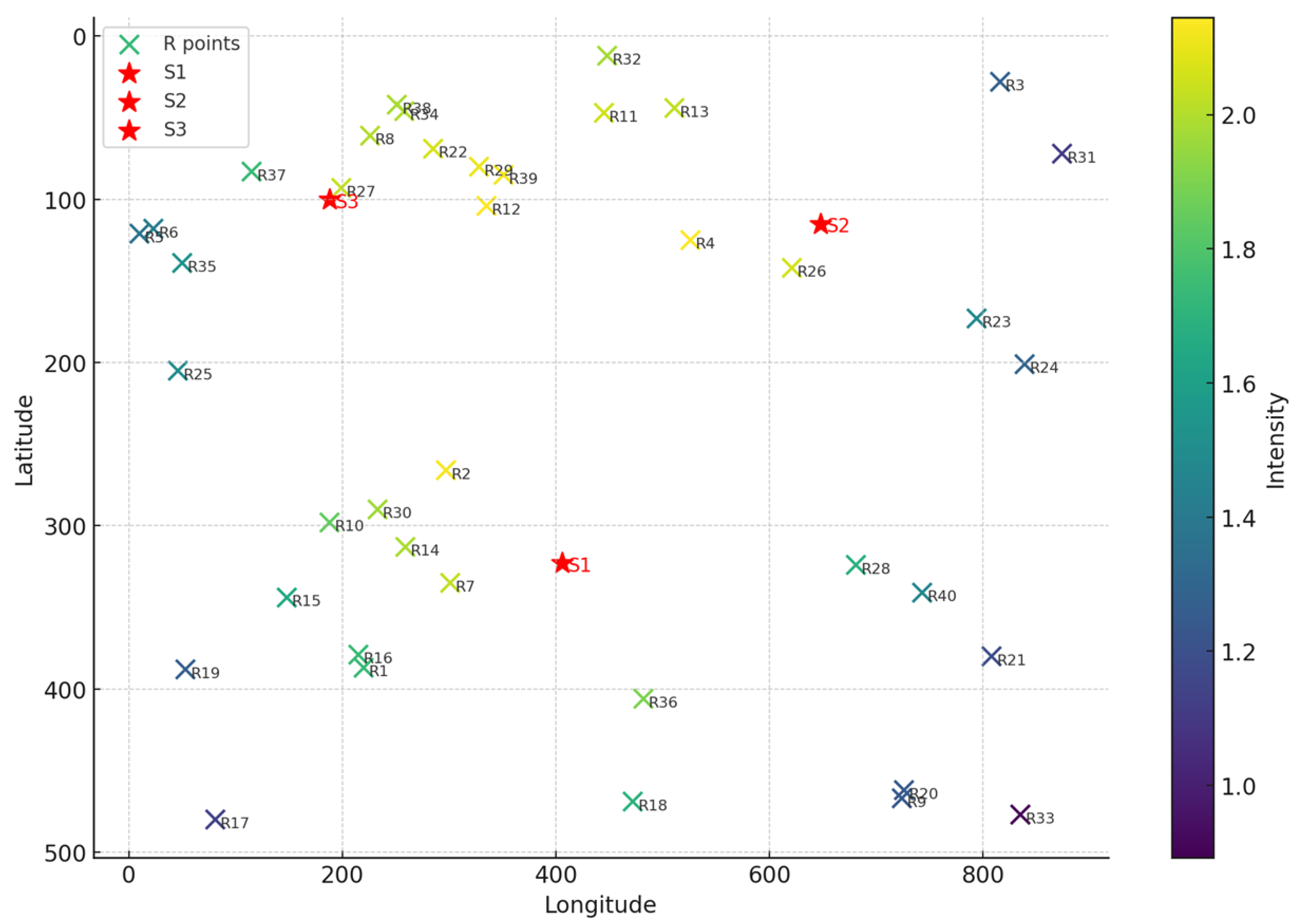
Experiment 5—Position of the points (receivers and sources). The last three rows report the coordinates of the hidden signal source, which is unknown to the algorithms under evaluation.
Table A9.
Experiment 5—Position of the points (receivers and sources). The last three rows report the coordinates of the hidden signal source, which is unknown to the algorithms under evaluation.
Type
Entity
Longitude
Latitude
Intensity
Data
R1
220
387
1.7341
Data
R2
297
266
2.1268
Data
R3
816
28
1.2805
Data
R4
526
125
2.1415
Data
R5
10
121
1.3683
Data
R6
23
118
1.4177
Data
R7
301
335
2.0267
Data
R8
226
61
1.9989
Data
R9
724
467
1.2364
Data
R10
188
298
1.8430
Data
R11
445
47
2.0567
Data
R12
335
104
2.1448
Data
R13
511
44
2.0228
Data
R14
259
313
1.9845
Data
R15
148
344
1.6479
Data
R16
215
379
1.7424
Data
R17
81
480
1.1396
Data
R18
472
469
1.6953
Data
R19
53
388
1.2733
Data
R20
726
462
1.2443
Data
R21
808
380
1.1860
Data
R22
285
69
2.0651
Data
R23
794
173
1.4747
Data
R24
839
201
1.2917
Data
R25
46
205
1.5010
Data
R26
621
142
2.0581
Data
R27
199
93
2.0339
Data
R28
681
324
1.6859
Data
R29
328
80
2.1066
Data
R30
233
290
1.9663
Data
R31
874
72
1.1156
Data
R32
448
12
1.9778
Data
R33
835
477
0.8922
Data
R34
258
46
1.9979
Data
R35
50
139
1.5302
Data
R36
482
406
1.8982
Data
R37
115
83
1.7429
Data
R38
251
42
1.9820
Data
R39
351
85
2.1230
Data
R40
743
341
1.4690
Hidden Source
S1
406
323
-
Hidden Source
S2
648
115
-
Hidden Source
S3
188
100
-
Figure A9.
The map representing the data of Table A9. The red color shows the position of the hidden source transmitting the signal.
Figure A9.
The map representing the data of Table A9. The red color shows the position of the hidden source transmitting the signal.
Table A10.
Quality measures for Experiment 5. The table shows, for each algorithm, the probability range in which the source is located (in bold), the fraction of area covered by the probability zone, and the corresponding quality score (corresponding to the bold entries).
Table A10.
Quality measures for Experiment 5. The table shows, for each algorithm, the probability range in which the source is located (in bold), the fraction of area covered by the probability zone, and the corresponding quality score (corresponding to the bold entries).
Bin Min
Bin Max
Mean
LC Extent
LC Precis.
PProb Extent
PProb Precis.
MLP Extent
MLP Precis.
SVCm Extent
SVCm Precis.
0.00
0.05
0.025
0.11775
0.02206
0.08183
0.02295
0.23705
0.01907
0.06858
0.02329
0.05
0.10
0.075
0.07765
0.06918
0.10823
0.06688
0.08913
0.06832
0.05753
0.07069
0.10
0.15
0.125
0.06113
0.11736
0.09558
0.11305
0.06718
0.11660
0.05423
0.11822
0.15
0.20
0.175
0.05598
0.16520
0.08508
0.16011
0.05518
0.16534
0.06008
0.16449
0.20
0.25
0.225
0.05300
0.21308
0.09545
0.20352
0.04878
0.21403
0.06095
0.21129
0.25
0.30
0.275
0.05070
0.26106
0.09333
0.24934
0.04123
0.26366
0.05958
0.25862
0.30
0.35
0.325
0.05575
0.30688
0.06150
0.30501
0.03495
0.31364
0.06818
0.30284
0.35
0.40
0.375
0.06625
0.35016
0.04643
0.35759
0.03115
0.36332
0.05310
0.35509
0.40
0.45
0.425
0.06240
0.39848
0.03758
0.40903
0.02895
0.41270
0.05060
0.40350
0.45
0.50
0.475
0.05708
0.44789
0.03320
0.45923
0.02813
0.46164
0.04750
0.45244
0.50
0.55
0.525
0.04470
0.50153
0.03303
0.50766
0.02825
0.51017
0.04483
0.50147
0.55
0.60
0.575
0.04510
0.54907
0.04078
0.55155
0.02690
0.55953
0.04210
0.55079
0.60
0.65
0.625
0.04388
0.59758
0.03338
0.60414
0.02768
0.60770
0.03903
0.60061
0.65
0.70
0.675
0.04065
0.64756
0.02905
0.65539
0.02735
0.65654
0.03803
0.64933
0.70
0.75
0.725
0.03333
0.70084
0.02723
0.70526
0.02840
0.70441
0.04038
0.69573
0.75
0.80
0.775
0.02900
0.75253
0.02830
0.75307
0.03008
0.75169
0.04765
0.73807
0.80
0.85
0.825
0.02893
0.80114
0.02488
0.80448
0.03278
0.79796
0.03985
0.79212
0.85
0.90
0.875
0.03423
0.84505
0.02043
0.85713
0.03770
0.84201
0.04145
0.83873
0.90
0.95
0.925
0.02983
0.89741
0.01660
0.90965
0.04463
0.88372
0.04510
0.88328
0.95
1.00
0.975
0.01770
0.95774
0.01318
0.96215
0.05955
0.91694
0.04630
0.92986
Figure A10.
Experiment 5—Scalar probability field computed by the algorithms. Color gradients in the heat map indicate values from maximum (deep red) to minimum (deep blue). From left to right and from top to bottom: (a) Linear Correlation; (b) Prior Probability; (c) Multilayer Perceptron; and (d) Supervised Contractive Map.
Figure A10.
Experiment 5—Scalar probability field computed by the algorithms. Color gradients in the heat map indicate values from maximum (deep red) to minimum (deep blue). From left to right and from top to bottom: (a) Linear Correlation; (b) Prior Probability; (c) Multilayer Perceptron; and (d) Supervised Contractive Map.
Appendix A.2. Analytical Formulation of the Supervised Contractive Map (SV-Cm)
This appendix summarizes the analytical formulation of the Supervised Contractive Map (SV-Cm), a bi-chamber supervised neural network characterized by harmonic activation and contractive learning dynamics.
Appendix A.2.1. Network Architecture
SV-Cm is a multilayer feed-forward neural network where each hidden neuron is composed of two computational chambers:
(i)
A classical chamber computing the weighted input;
(ii)
A contractive chamber measuring the deviation of weights from a structural constant.
The interaction of these chambers produces a harmonically modulated activation.
Appendix A.2.2. Notation
The following notation is adopted throughout this appendix:
l: the layer index;
i: the neuron index;
: the output of neuron i in layer l;
: the weight connecting neuron j (layer ) to neuron i (layer l);
: the number of neurons in layer l.
Appendix A.2.3. Forward Propagation
The classical net input for neuron i in layer l is defined as
The contractive net input is
The bi-chamber activation combines both components through a sinusoidal modulation:
Appendix A.2.4. Loss Function
The supervised training objective is the quadratic prediction error:
where denotes the target value for output neuron i. Although this loss defines the prediction objective, the weight dynamics of SV-Cm cannot be expressed purely as the gradient of this function because of the contractive factor.
Appendix A.2.5. Backward Propagation
The output layer error is
The hidden layer error is
Appendix A.2.6. Contractive Weight Update
The weight update rule incorporates a contractive factor, as follows:
where denotes the learning coefficient. This contractive factor introduces a geometric constraint in weight space, automatically limiting weight growth and stabilizing the learning dynamics.
Appendix A.2.7. Conceptual Implications
SV-Cm combines supervised error minimization with an intrinsic contractive mechanism that regulates weight magnitude. The harmonic modulation induced by the sinusoidal activation enables the network to represent highly nonlinear decision boundaries while maintaining stable learning dynamics. This property makes SV-Cm particularly suitable for the source localization task addressed by the TWC Sigma framework, where the neural network must learn the complex spatial relationships between observation points and hidden sources.
Appendix B
Appendix B.1. Monte Carlo Null Tests for the Spatial Improbability of the SVCm Radiation Map
Appendix B.1.1. Rationale
To assess whether the spatial configuration highlighted by the SVCm recall map could plausibly arise by chance from the empirical dataset, we performed a set of Monte Carlo null model analyses. The purpose of these tests was not to reproduce the full SVCm learning-and-recall procedure pixel by pixel, but rather to address a more fundamental issue: whether the observed relationship between the geographic coordinates of the measurement sites and the recorded radiation intensity values is compatible with a random allocation of the signal over the sampled locations.
The null hypothesis was defined as follows: the set of spatial coordinates remains fixed, whereas the radiation intensity values (Power) are randomly reassigned across the 3467 sampling points. Under this hypothesis, any coherent source-like spatial organization should disappear, and any apparent offshore hotspot should be attributable to chance alone.
Appendix B.1.2. Dataset
The analysis was based on the empirical dataset used in the main study, consisting of 3467 observation points. Each record included four variables: an ID code, longitude, latitude, and radiation intensity (Power). Formally, each observation can be represented as and , where denotes the geographic location of the i-th sampling site, and denotes the associated signal intensity.
The tests were designed to preserve the exact spatial geometry of the sample while destroying any true spatial correspondence between position and signal amplitude.
Appendix B.1.3. Null Model and Monte Carlo Procedure
A Monte Carlo procedure with randomizations was adopted. For each replication, the Power values were randomly permuted across the 3467 fixed geographic locations, thereby generating a surrogate dataset in which the marginal distribution of the observed signal was perfectly preserved, but its spatial organization was removed. This procedure produces a conservative null model because it leaves the following unchanged: (1) the number of sampled points, (2) the exact geometry of the sampled locations, and (3) the full empirical distribution of radiation values. Only the association between location and signal intensity is broken. Three complementary tests were then performed.
Appendix B.1.4. Test 1: Global Search for a Source-Like Spatial Attractor
A grid search was performed over the study area. For each candidate spatial point , the Euclidean distance was computed to every observed site. The relationship between these distances and the observed signal values was quantified by computing . The candidate point yielding the strongest negative association was retained: if a genuine source exists, the signal intensity should decrease with increasing distance from that source. The same procedure was repeated for each of the 100 Monte Carlo randomizations.
In the empirical dataset, the best candidate point was found offshore, east of Japan, consistent with the SVCm recall map. The minimum observed correlation was . Under the null model, the corresponding values were centered near zero (null mean: ; null SD: ; and null range: approximately ). No Monte Carlo replicate approached the empirical value, yielding and a z-score of approximately .
Appendix B.1.5. Test 2: Distance–Signal Association at the Point Highlighted by the SVCm Map
A second test was performed using the specific point emphasized in the SVCm map, approximately located at 38.3° N and 142.4° E. For this fixed point , the statistic was evaluated for the empirical dataset and for all 100 surrogates.
In the real data, the correlation was . Under the null model, the null mean , null SD , and null range . The observed value was well outside the null interval (; ). The offshore point emphasized by the SVCm recall map therefore corresponds to a location from which the empirical field shows a strong and highly significant radial decay pattern, entirely absent in the randomized datasets.
Appendix B.1.6. Test 3: Radial Concentration of Signal Around the Best Source Proxy
All observation points were ranked by their distance from the best source proxy identified in Test 1. The proportion of total signal mass within the closest 1%, 5%, and 10% of points was computed. The empirical dataset showed strong radial concentration: closest 1%: 12.5% of total signal; closest 5%: 40.8%; closest 10%: 54.7%. Under the null model, corresponding values were much lower (1%: ∼1.1%; 5%: ∼5.1%; 10%: ∼10.1%), and the observed concentrations exceeded the entire Monte Carlo null distribution in all cases ().
Appendix B.1.7. Summary and Conclusions
The three null tests converge on the same conclusion. The empirical dataset exhibits a strong and highly non-random spatial organization: (1) there exists an offshore point that maximizes a negative distance–signal relationship far beyond null expectation; (2) the specific point emphasized in the SVCm recall map shows a highly significant radial decay of signal; and (3) the total radiation field is sharply concentrated around the inferred source region in a way incompatible with random signal placement. In all tests, empirical results lay far outside the range generated by 100 Monte Carlo randomizations.
It is important to clarify the inferential scope: these tests do not constitute a full replication of the SVCm training and recall process over the grid. They validate a more basic premise—the empirical dataset contains a highly significant source-like spatial organization incompatible with random redistribution of signal values over the sampled coordinates. A complete null validation of the entire SVCm pipeline would require retraining on each surrogate dataset and comparing recall maps via explicit map-level statistics. However, the present analyses already provide strong evidence that the source-like pattern revealed by the empirical map is highly improbable under a null model of random spatial assignment.
References
Sterchi, M.; Hilfiker, L.; Grütter, R.; Bernstein, A. Active Querying Approach to Epidemic Source Detection on Contact Networks. Sci. Rep.2023, 13, 11363. [Google Scholar] [CrossRef] [PubMed]
Li, X.; Wang, X.; Zhao, C.; Zhang, X.; Yi, D. Locating the Epidemic Source in Complex Networks with Sparse Observers. Appl. Sci.2019, 9, 3644. [Google Scholar] [CrossRef]
Choi, J. Epidemic Source Detection over Dynamic Networks. Electronics2020, 9, 1018. [Google Scholar] [CrossRef]
Biazzo, I.; Braunstein, A.; Dall’Asta, L.; Mazza, F. A Bayesian Generative Neural Network Framework for Epidemic Inference Problems. Sci. Rep.2022, 12, 19673. [Google Scholar] [CrossRef] [PubMed]
Shah, C.; Dehmamy, N.; Perra, N.; Chinazzi, M.; Barabási, A.-L.; Vespignani, A.; Yu, R. Finding Patient Zero: Learning Contagion Source with Graph Neural Networks. arXiv2020, arXiv:2006.11913. [Google Scholar] [CrossRef]
Chen, Y.; Volić, I. Topological Data Analysis Model for the Spread of the Coronavirus. PLoS ONE2021, 16, e0255584. [Google Scholar] [CrossRef] [PubMed]
Taylor, D.; Klimm, F.; Harrington, H.A.; Kramár, M.; Mischaikow, K.; Porter, M.A.; Mucha, P.J. Topological Data Analysis of Contagion Maps for Examining Spreading Processes on Networks. Nat. Commun.2015, 6, 7723. [Google Scholar] [CrossRef] [PubMed]
Tan, C.W.; Yu, P.-D. Contagion Source Detection in Epidemic and Infodemic Outbreaks: Mathematical Analysis and Network Algorithms. Found. Trends Netw.2023, 13, 107–251. [Google Scholar] [CrossRef]
Buscema, M.; Asadi-Zeydabadi, M.; Massini, G.; Lodwick, W.A.; Breda, M.; Petritoli, R.; Newman, F.; Della Torre, F. The Topological Weighted Centroid: A New Vision of Geographic Profiling: Theory and Applications; Springer: Cham, Switzerland, 2023; Volume 1095. [Google Scholar]
Hamaoka, Y. Validating Citizen-Led Radioactivity Measurement: “Minna-No Data Site”; Social Science Research Network: Rochester, NY, USA, 2025. [Google Scholar] [CrossRef]
Minna-No Data Site. Official Website. Minna-No Data Site 2025. Available online: https://en.minnanods.net (accessed on 22 July 2025).
Buesseler, K. Fukushima and Ocean Radioactivity. Oceanography2014, 27, 92–105. [Google Scholar] [CrossRef]
Honda, M.C.; Kawakami, H.; Watanabe, S.; Saino, T. Concentration and Vertical Flux of Fukushima-Derived Radiocesium in Sinking Particles from Two Sites in the Northwestern Pacific Ocean. Biogeosciences2013, 10, 3525–3534. [Google Scholar] [CrossRef]
Kaeriyama, H. 134Cs and 137Cs in the Seawater Around Japan and in the North Pacific. In Impacts of the Fukushima Nuclear Accident on Fish and Fishing Grounds; Nakata, K., Sugisaki, H., Eds.; Springer: Tokyo, Japan, 2015; pp. 11–32. [Google Scholar] [CrossRef]
Figure 1.
Geographical map displaying the sites where measurements were conducted; the observation points are marked in red.
Figure 1.
Geographical map displaying the sites where measurements were conducted; the observation points are marked in red.
Figure 2.
Experiment 6a—Scalar probability field computed by TWC Sigma using Linear Correlation. Color gradients in the heat map indicate values from maximum (deep red) to minimum (deep blue).
Figure 2.
Experiment 6a—Scalar probability field computed by TWC Sigma using Linear Correlation. Color gradients in the heat map indicate values from maximum (deep red) to minimum (deep blue).
Figure 3.
Experiment 6b—Scalar probability field computed by TWC Sigma using Prior Probability. Color gradients in the heat map indicate values from maximum (deep red) to minimum (deep blue).
Figure 3.
Experiment 6b—Scalar probability field computed by TWC Sigma using Prior Probability. Color gradients in the heat map indicate values from maximum (deep red) to minimum (deep blue).
Figure 4.
Experiment 6c—Scalar probability field computed by TWC Sigma using Multilayer Perceptron. Color gradients in the heat map indicate values from maximum (deep red) to minimum (deep blue).
Figure 4.
Experiment 6c—Scalar probability field computed by TWC Sigma using Multilayer Perceptron. Color gradients in the heat map indicate values from maximum (deep red) to minimum (deep blue).
Figure 5.
Experiment 6d—Scalar probability field computed by TWC Sigma using Supervised Contractive Map. Color gradients in the heat map indicate values from maximum (deep red) to minimum (deep blue).
Figure 5.
Experiment 6d—Scalar probability field computed by TWC Sigma using Supervised Contractive Map. Color gradients in the heat map indicate values from maximum (deep red) to minimum (deep blue).
Disclaimer/Publisher’s Note: The statements, opinions and data contained in all publications are solely those of the individual author(s) and contributor(s) and not of MDPI and/or the editor(s). MDPI and/or the editor(s) disclaim responsibility for any injury to people or property resulting from any ideas, methods, instructions or products referred to in the content.
Buscema, P.M.; Breda, M.; Petritoli, R.; Massini, G.; Ferilli, G.
The TWC Sigma Model: A Nonlinear Correlation and Neural Network Approach for Spatial Source Detection. J. Exp. Theor. Anal.2026, 4, 16.
https://doi.org/10.3390/jeta4020016
AMA Style
Buscema PM, Breda M, Petritoli R, Massini G, Ferilli G.
The TWC Sigma Model: A Nonlinear Correlation and Neural Network Approach for Spatial Source Detection. Journal of Experimental and Theoretical Analyses. 2026; 4(2):16.
https://doi.org/10.3390/jeta4020016
Chicago/Turabian Style
Buscema, Paolo Massimo, Marco Breda, Riccardo Petritoli, Giulia Massini, and Guido Ferilli.
2026. "The TWC Sigma Model: A Nonlinear Correlation and Neural Network Approach for Spatial Source Detection" Journal of Experimental and Theoretical Analyses 4, no. 2: 16.
https://doi.org/10.3390/jeta4020016
APA Style
Buscema, P. M., Breda, M., Petritoli, R., Massini, G., & Ferilli, G.
(2026). The TWC Sigma Model: A Nonlinear Correlation and Neural Network Approach for Spatial Source Detection. Journal of Experimental and Theoretical Analyses, 4(2), 16.
https://doi.org/10.3390/jeta4020016
Article Metrics
No
No
Article Access Statistics
Multiple requests from the same IP address are counted as one view.
Buscema, P.M.; Breda, M.; Petritoli, R.; Massini, G.; Ferilli, G.
The TWC Sigma Model: A Nonlinear Correlation and Neural Network Approach for Spatial Source Detection. J. Exp. Theor. Anal.2026, 4, 16.
https://doi.org/10.3390/jeta4020016
AMA Style
Buscema PM, Breda M, Petritoli R, Massini G, Ferilli G.
The TWC Sigma Model: A Nonlinear Correlation and Neural Network Approach for Spatial Source Detection. Journal of Experimental and Theoretical Analyses. 2026; 4(2):16.
https://doi.org/10.3390/jeta4020016
Chicago/Turabian Style
Buscema, Paolo Massimo, Marco Breda, Riccardo Petritoli, Giulia Massini, and Guido Ferilli.
2026. "The TWC Sigma Model: A Nonlinear Correlation and Neural Network Approach for Spatial Source Detection" Journal of Experimental and Theoretical Analyses 4, no. 2: 16.
https://doi.org/10.3390/jeta4020016
APA Style
Buscema, P. M., Breda, M., Petritoli, R., Massini, G., & Ferilli, G.
(2026). The TWC Sigma Model: A Nonlinear Correlation and Neural Network Approach for Spatial Source Detection. Journal of Experimental and Theoretical Analyses, 4(2), 16.
https://doi.org/10.3390/jeta4020016





 ,
,