A Hybrid Whale Optimization Approach for Fast-Convergence Global Optimization

Abstract

In this paper, we introduce the Levy Flight-enhanced Whale Optimization Algorithm with Tabu Search elements (LWOATS), an innovative hybrid optimization approach that enhances the standard Whale Optimization Algorithm (WOA) with advanced local search techniques and elite solution management to improve performance on global optimization problems. Techniques from the Tabu Search algorithm are adopted to balance the exploration and exploitation phases, while an elite reintroduction strategy is implemented to retain and refine the best solutions. The efficient optimization of LWOATS is further aided by the utilization of Levy flights and local search based on the Nelder–Mead simplex method. An Orthogonal Experimental Design (OED) analysis was employed to fine-tune the algorithm’s parameters. LWOATS was tested against three different algorithm sets: fundamental algorithms, advanced Differential Evolution (DE) variants, and improved WOA variants. Wilcoxon tests demonstrate the promising performance of LWOATS, showing improvements in convergence speed, accuracy, and robustness compared to traditional WOA and other metaheuristic algorithms. After extensive testing against a challenging set of benchmark functions and engineering optimization problems, we conclude that our proposed method is well suited for tackling high-dimensional optimization tasks and constrained optimization problems, providing substantial computational efficiency gains and improved overall solution quality.

1. Introduction

Modern engineering, computational science, and energy management applications increasingly hinge on solving complex optimization tasks driven by large datasets and sophisticated simulation models [1,2,3]. Classical gradient-based and direct search methods falter when confronted with non-continuous or non-differentiable objectives in high-dimensional spaces. Landscapes are littered with dozens or even hundreds of local optima, in which such methods routinely become trapped [4].

Global optimization instead seeks the absolute best value (the minimum or maximum) of a real-valued function over its entire feasible region, regardless of non-convexity, discontinuities, or complex inequality/equality constraints. The challenge deepens when evaluations come from expensive black box simulations, noisy measurements, or very large parameter vectors, since analytical solutions are unavailable and brute force search is impractical. To overcome these hurdles, metaheuristic algorithms (many inspired by natural processes) combine stochastic exploration with adaptive exploitation to locate near-global optima under tight evaluation budgets [5].

Metaheuristic optimization is typically the method of choice when design spaces are discontinuous, multimodal, or prohibitively costly for gradient-based solvers. Early exemplars, including particle swarm optimization (PSO) [6], Ant Colony Optimization (ACO) [7], and the genetic algorithm (GA) [8,9] borrowed simple behavioral rules from flocking, pheromone foraging, and natural selection to balance exploration and exploitation. Subsequent nature-inspired variants refined that balance through different metaphors: echolocation in the Bat Algorithm (BA) [10], pack hierarchy in Grey Wolf Optimization (GWO) [11], and cross-patch pollination in the flower pollination algorithm (FPA) [12]. In parallel, the Differential Evolution (DE) lineage introduced adaptive parameter control with algorithms such as JaDE [13], SHADE and L-SHADE [14,15], iL-SHADE [16], and the current CEC leader jSO [17], showing that tighter population management can boost robustness across benchmark suites.

A complementary way to strengthen a metaheuristic is to equip it with memory. Tabu Search (TS) records recently visited states, discouraging the algorithm from cycling and encouraging fresh exploration. Modern hybrids demonstrate the versatility of this idea: quantum-assisted TS cracks large asymmetric TSP instances [18], TS combined with network flow optimizers improves multi-objective supply chain design [19], TS with iterated local search yields high-quality sports timetables [20], and TS fused with quantum routines accelerates multi-objective searches [21]. Collectively, these studies indicate that a lightweight tabu layer can sharpen global search without sacrificing the intensification strengths of swarms or evolutionary engines (a principle we adopt in the present work).

The bio-inspired Whale Optimization Algorithm (WOA) [22] models humpback whales’ bubble-net hunting to alternate between global exploration and local exploitation, and has been successfully applied to structural design [23,24], image processing [25], network topology [26,27,28], and scheduling [29,30]. Yet, like many metaheuristics, WOA can converge slowly on flat or narrow ridges and tends to stagnate in multimodal basins. To overcome these limitations, two main trajectory enrichment strategies have emerged. Some studies graft Levy flight perturbations onto WOA (LWOA) to enable occasional long jumps that escape deep local minima [31,32] while others use chaotic map sequences to inject deterministic yet unpredictable fluctuations into the position updates, preserving population diversity and preventing premature convergence [33,34]. These enhancements accelerate convergence on benchmark functions by widening the search radius early on and maintaining exploration pressure as the swarm contracts. A taxonomy of these enhancements and hybridization strategies is illustrated in Figure 1.

Beyond enriching trajectories, hybridization with complementary metaheuristics has been widely explored. Velocity–position rules from PSO have been embedded in WOA to introduce inertia effects and momentum memory [35,36], while Grey Wolf Optimization’s leadership hierarchy has been combined with bubble-net encircling to improve exploitation in high-dimensional spaces [37]. Local search modules (ranging from Nelder–Mead simplices to Tabu Search) provide deterministic intensification around elite solutions, sharpening final convergence [38]. These hybrid frameworks demonstrate robust gains across diverse applications, from optimizing truss structures [23] and gear trains to robotic path planning [39,40], yet each typically addresses only one weakness of WOA. A truly integrated approach that unites long-jump exploration, memory-guided diversification, and deterministic local refinement remains lacking, motivating the design of LWOATS in this work.

In this work, we propose a hybrid Whale Optimization Algorithm (WOA) that integrates components from Levy flights, the Nelder–Mead simplex, and Tabu Search for solving global optimization problems, with a particular focus on engineering applications. Levy flights inject rare long jumps that help escape deep local minima, the Tabu Search memory layer prevents wasted revisits and sustains diversity, and Nelder–Mead local refinement rapidly hones in on the most promising regions. By directly addressing WOA’s weaknesses (premature convergence, cycling, and slow exploitation), LWOATS is designed to converge more quickly, achieve statistically superior optima under a fixed evaluation budget, and generalize robustly to unseen high-dimensional benchmarks and constrained engineering problems. We conducted extensive evaluations using 23 benchmark functions, comparing the performance of our algorithm, LWOATS, against a wide range of algorithms, including fundamental methods like PSO, GWO, DE, and WOA and top-performing algorithms from CEC competitions, such as JaDE, SHADE, iL-SHADE, jSO, as well as enhanced WOA variants. The results demonstrate that LWOATS not only achieves a competitive performance but also outperforms these algorithms in most cases. Wilcoxon statistical tests further validate the superiority of our approach, as evidenced by significantly low p-values. The novelty of LWOATS lies in its use of memory elements, which prevent the algorithm from revisiting poor search areas while guiding it toward more promising regions. This mechanism enables LWOATS to find the global optimum with fewer evaluations compared to other algorithms. Moreover, LWOATS excels in solving difficult problems, such as Shekel’s functions, where many other algorithms struggle. Finally, LWOATS’s exceptional performance extends to engineering optimization problems, where it consistently delivers the best solutions compared to existing approaches in the literature.

The rest of this paper is structured as follows: Section 2 is a brief summarization of all the theory and mathematics that lay behind LWOATS and that are needed to understand its functionality. Section 3 includes the evaluation results of LWOATS on well-known benchmark functions as they are declared in the literature. LWOATS is compared with fundamental algorithms but also with advanced DE variations and with other improved versions of WOA. In Section 4, LWOATS is applied in various constrained engineering problems, and the driven results are compared with the ones from other metaheuristic approaches. Finally, through Section 5, the findings of this work are summarized, and various directions for future work are suggested.

2. Background

2.1. Whale Optimization Algorithm

Inspired by the cooperative hunting of humpback whales, WOA alternates three behaviors: (i) search/exploration, where whales move randomly across the search space to sample diverse regions; (ii) encircling, in which all individuals adaptively contract toward the best solution found so far; and (iii) the bubble-net attack (exploitation), modeled either by a shrinking circle update or by a logarithmic spiral trajectory that tightens around the prey (see Figure 2). Equation (2) models this behavior:

$$\begin{array}{c}\hfill {\overrightarrow{D}}^{\prime }=|{\overrightarrow{X}}^{\ast }\left(t\right)-\overrightarrow{X}\left(t\right)|\end{array}$$

(1)

$$\begin{array}{c}\hfill \overrightarrow{X}(t+1)={\overrightarrow{D}}^{\prime }·e^{b·l}·cos\left(2\pi l\right)+{\overrightarrow{X}}^{\ast }\left(t\right),\end{array}$$

(2)

where b and l follow the original settings of Mirjalili and Lewis [22].

Together, these operators balance global exploration with local intensification and have proved competitive on many continuous optimization tasks. Full derivations of the random search and encircling operators are given in Appendix A.

2.2. Nelder–Mead Simplex

The Nelder–Mead simplex algorithm is a widely used derivative-free optimization method for minimizing a multi-variable function without the need for derivatives. It was first proposed by Nelder and Mead in 1965 [41]. The main idea of this algorithm is that it defines a polyhedron with $n+1$ vertices, $x_0,x_1,\dots ,x_n\in {\mathbb{R}}^n$ (simplex $S\in {\mathbb{R}}^n$) in the n-dimensional search space. These $n+1$ vertices are evaluated on the objective function $f:{\mathbb{R}}^n\to \mathbb{R}$ and sorted based on the result. In each iteration, the algorithm accesses this solution and determines the worst $x_h={max}_j{x}_j$, the second worst $x_s={max}_{j\ne h}{x}_j$, and the best $x_l={min}_{j\ne h}{x}_j$, point. The centroid of this structure is calculated based on the following equation:

$$x_c:={\displaystyle \frac{1}{n}}\sum _{i\ne h}{x}_i$$

(3)

Then, a number of transformations take place until the termination criteria are met (e.g., the simplex size falling below a threshold or reaching a maximum number of iterations) and the optimization process stops. More particularly, at every iteration, the worst vertex is reflected about the simplex centroid and, if beneficial, expanded. Otherwise, the algorithm contracts or shrinks the simplex toward the current best point. These four affine transformations, namely, reflection, expansion, contraction, and shrink, give NM fast convergence on smooth bowls and make it a popular intensification kernel in hybrid metaheuristics. Formal update formulas and the centroid expression are listed in Appendix B.

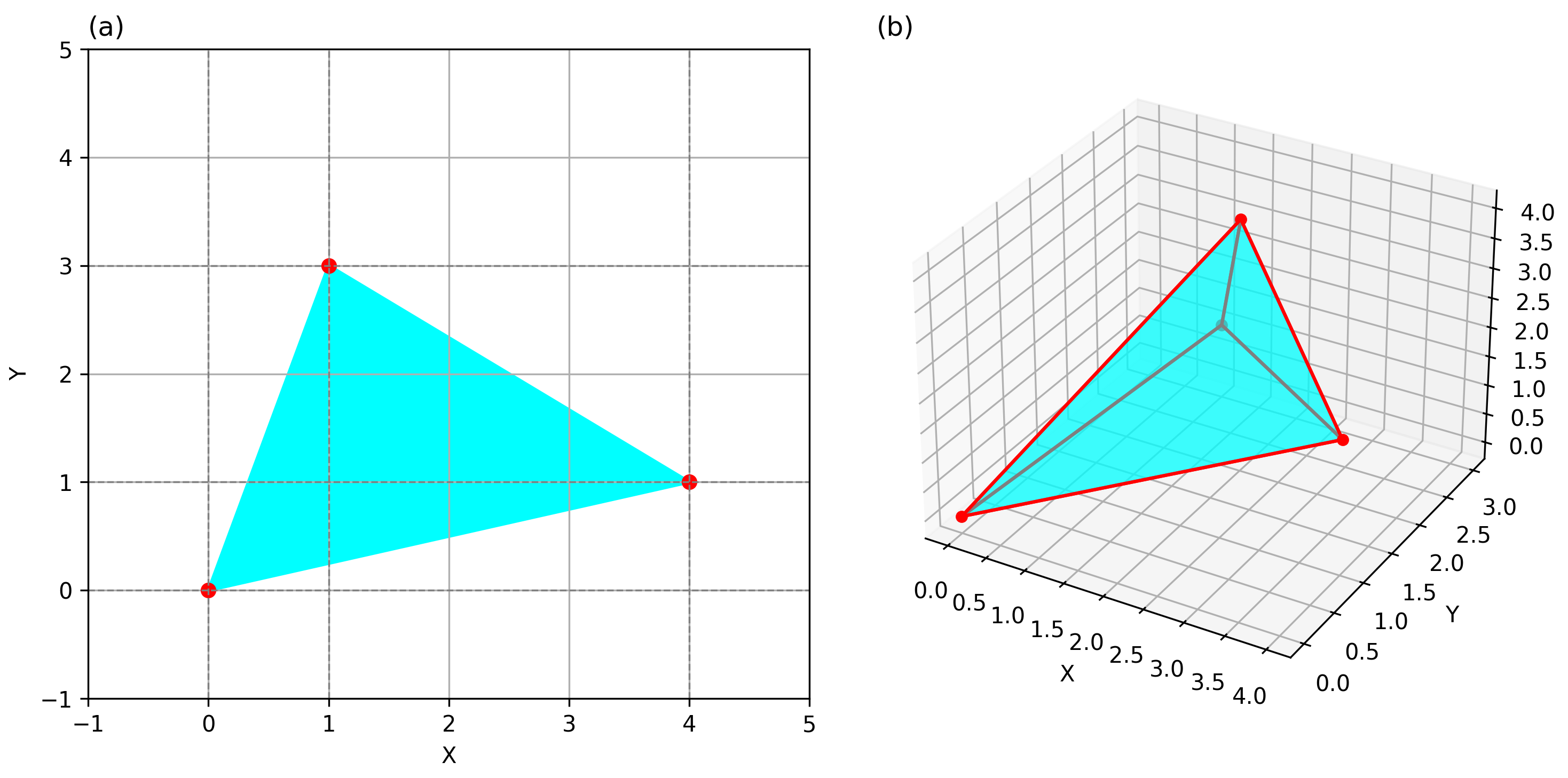
As illustrated in Figure 3, a 2D simplex is represented by a triangle, while a 3D simplex is represented by a tetrahedron, each vertex of which serves as a potential solution in the optimization process.

Numerous studies have showcased the potential of the integration of Nelder–Mead simplex strategies in other metaheuristic algorithms. In [42], a continuous hybrid algorithm (CHA) that strategically combines genetic algorithms (GAs) with the Nelder–Mead simplex search (SS) is proposed. The hybrid algorithm employs GAs for the initial exploratory phase of the optimization process, leveraging their ability to efficiently search large and complex landscapes for promising regions (exploration). Once these regions are identified, the Nelder–Mead takes over to perform a more focused and fine-grained search to accurately determine the optimal values within these regions (exploitation).

The same design philosophy (broad, population-based exploration followed by a sharp deterministic refiner) has proved successful in several recent hybrids. Solaiman et al. [43] fuse Newton’s second-order update with the Sperm Swarm Optimizer, producing the MSSO hybrid that solves eight nonlinear equation systems, including three real-world models in chemistry and neurophysiology, and outperforms SSO, HHO, BOA, ALO, PSO, and EO in terms of stability, final fitness, and convergence speed. In a complementary study, Sarı et al. [44] embed Newton–Raphson updates inside the Harris hawks optimizer to create NHHO, which outperforms HHO, PSO, ALO, BOA, and EO on six benchmark nonlinear systems by achieving smaller equation norms and quicker convergence. Both works underline our design choice in LWOATS: a deterministic second-order (or derivative-free) local search module can substantially boost a swarm’s accuracy and speed, particularly when the objective involves stiff or highly coupled nonlinear relationships.

A similar approach is followed in [45], where a hybrid algorithm HCSNM, that integrates the cuckoo search (CS) with the Nelder–Mead, is introduced. Initially, the standard cuckoo search algorithm is used to perform a global search, characterized by its Levy flights, promoting a broad and diverse exploration of the search space. After several iterations, the best solution found by the CS is then used as a starting point for the Nelder–Mead algorithm. This shift marks a transition to a local search or intensification phase aimed at refining the solution by exploring its immediate neighborhood more thoroughly. This enhances the standard CS by reducing its tendency toward slow convergence and improving its efficiency in finding optimal or near-optimal solutions. Among these, other hybridization strategies include integration with PSO [46,47,48], DE [49,50], SA [51], TS [52], and others.

2.3. Tabu Search Algorithm

The Tabu Search (TS) algorithm is a single-trajectory metaheuristic method initially proposed in [53] that mimics the behavior of human thinking. TS improves a solution by exploring its neighborhood but forbids immediate returns to recently visited states via an adaptive “tabu” memory [53,54]. We embed TS because WOA can revisit the same basins once its population loses diversity. The tabu mechanism breaks such cycles with negligible overhead and almost no extra hyper-parameters. In addition, a long-term elite list retains the best candidates and periodically re-injects them for focused refinement, providing synergy with Nelder–Mead’s local search.

The core principles of TS can be described by two primary types of memory elements:

• Memory tiers.
  • Tabu list (length k): blocks the last k accepted moves, steering exploration into new regions.
  • Elite list (size m): archives the top-m solutions to safeguard global information and guide intensification.

The TS algorithm can be formulated mathematically. Let us denote with $\mathcal{T}$ the tabu list. This list can be represented as

$$\mathcal{T}=\{{\overrightarrow{x}}_1,{\overrightarrow{x}}_2,\dots ,{\overrightarrow{x}}_n\},$$

(4)

where ${\overrightarrow{x}}_i$ is the $i_{th}$ recently visited solution vector. In a typical TS algorithm, there is a move and an aspiration function. The “move” function $\mathcal{M}$ is the way the algorithm moves from one solution vector $\overrightarrow{x}$ to the next one ${\overrightarrow{x}}^{\ast }$. This function creates a new set of possible moves that can be applied to $\overrightarrow{x}$:

$$\mathcal{N}\left(\overrightarrow{x}\right)=\left\{{\overrightarrow{x}}^{\ast }\right|{\overrightarrow{x}}^{\ast }=\mathcal{M}(\overrightarrow{x},\overrightarrow{\delta }),\mathrm{where}\overrightarrow{\delta }\in D\},$$

(5)

where D represents possible solutions. The aspiration function $A({\overrightarrow{x}}^{\ast })$ is a Boolean function that returns true if $f({\overrightarrow{x}}^{\ast })<f({\overrightarrow{x}}^{\prime })$, where f is the objective function and ${\overrightarrow{x}}^{\prime }$ is the best solution so far. Each iteration of TS involves selecting a move from the neighborhood that minimizes the objective function while not being tabu, unless it meets the aspiration criteria:

$${\overrightarrow{x}}_{\mathrm{next}}=arg\underset{{\overrightarrow{x}}^{\ast }\in N(\overrightarrow{x})}{min}\{f({\overrightarrow{x}}^{\ast })\mid {\overrightarrow{x}}^{\ast }\notin \mathcal{T}\mathrm{or}A({\overrightarrow{x}}^{\ast })\mathrm{is}\mathrm{true}\}.$$

(6)

This is repeated until a termination criterion is met, such as a maximum number of iterations or a satisfactory solution quality. Through this approach, the search efficiently explores new areas while using its memory of past solutions in a smart way to avoid already searched solution spaces or less promising paths.

2.4. Levy Flights

Levy flights are essentially random walks that follow the Levy distribution. Even though they were first introduced by the French mathematician Levy, they were described more in depth later by Benoit Mandelbrot [55]. Following this distribution, an agent will make small steps until they eventually make larger steps or even a full rotation in their direction. Numerous studies have showcased that Levy flights are highly effective in optimizing stochastic and global optimization algorithms due to their ability to avoid local minima by enabling jumps to remote areas of the search space, enhancing the exploration capabilities of algorithms like PSO [56,57,58], CS [59], and ACO [60,61], among others. The equation for the Levy flights can be formulated as follows:

$$L\left(s\right)\sim u=t^{-\lambda },1<\lambda \le 3$$

(7)

A useful algorithm [4] that can simulate the Levy flights can be described by Equation (8):

$$s={\displaystyle \frac{\mu }{{\left|\nu \right|}^{1/\beta }}},$$

(8)

where $\mu \sim N(0,{\sigma }_{\mu }^2)$ and $\nu \sim N(0,{\sigma }_{\nu }^2)$, following the normal distribution, and $\beta =1.5$, ${\sigma }_{\nu }=1$ while ${\sigma }_{\mu }$, can be calculated by Equation (9):

$${\sigma }_{\mu }={\left[{\displaystyle \frac{\mathsf{\Gamma }(1+\beta )sin\left(\frac{\pi \beta }{2}\right)}{\mathsf{\Gamma }\left(\frac{1+\beta }{2}\right)\beta 2^{(\beta -1)/2}}}\right]}^{{\displaystyle \frac{1}{\beta }}}$$

(9)

With $\mathsf{\Gamma }$, we denote the gamma function which is defined by the integral: $\mathsf{\Gamma }\left(z\right)={\int }_0^{\infty }{t}^{z-1}{e}^{-t}dt$, and $z\in \mathbb{C}$, where $\mathcal{R}e\left(z\right)>0$.

2.5. Enhanced Whale Optimization Algorithm with Levy Flight and Tabu Search Features: LWOATS

WOA has showcased some good results in finding the best solution to various optimization problems; however, it has some limitations. The first deals with its susceptibility to premature convergence. This can seriously degrade the performance, especially in finding the global minimum, in highly dimensional, complex, and multimodal landscapes [62]. WOA further presents slow speeds of reaching convergence in some scenarios, complicating the landscape in time-sensitive or computationally intensive environments. Finally, another notable limitation includes the possibility of local optima stagnation, due to the limited exploration of the WOA, i.e., the algorithm’s search may stop if not enough diversity is maintained among the solutions [63].

To face some of these limitations, we propose LWOATS, a hybrid algorithm that enhances the exploitation phase of WOA using the Nelder–Mead simplex for Local Search and memory elements from TS to prevent the re-evaluation of best solutions and the exploration phase by Levy flights. More specifically, the exploration phase adopted by WOA is described by Equations (A1)–(A4). However, in each iteration, the new agent’s position $\overrightarrow{X}(t+1)$ is adapted based on a Levy flight with a specific scaling factor $\mathcal{F}$.

The incorporation of Levy flights in the position update mechanism of the algorithm significantly improves the exploration capabilities, thus allowing it to effectively escape from the probable local minima pitfalls in complex, multimodal fitness landscapes. The use of a small scaling factor with Levy flights tunes to a compromise between making extensive exploratory moves while leaving the current evolutionary trajectory of each agent largely intact. This allows the algorithm to search broadly when needed and be sensitive to the fine variations in the optimization problem. Moreover, such an approach portrays a high level of flexibility and adaptability since the algorithm by itself can dynamically set the intensity of exploration with respect to the outcomes derived from Levy flights. Such adaptability becomes relevant in cases where the objective function’s landscape is dynamic or ill understood, just to ensure the algorithm’s robustness across problem settings:

$$\overrightarrow{X}(t+1)=\overrightarrow{X}(t+1)\times s\times \mathcal{F},$$

(10)

where s is given by Equation (8) and the scaling factor is chosen to be $\mathcal{F}=0.01$ following the choice of [64].

Additionally, in LWOATS, we integrate Tabu Search strategies to increase its potential to escape repetitive and cyclic search, which is a failure in most complex optimization scenarios. WOA acts as the “move” function in our case and is used to determine the next possible moves in the search space (Equation (5)). Using a Tabu list that acts as a memory registering previously investigated solutions (Equation (4)), the algorithm naturally avoids searching these areas, ensuring that each step during the exploration is going to new regions of the solution space (Equation (6)). Thus, LWOATS avoids being trapped in local minima, a critical advantage when solving multimodal problems, while at the same time can cover much space more systematically and effectively due to the enhanced exploratory capabilities gained by the TS methods.

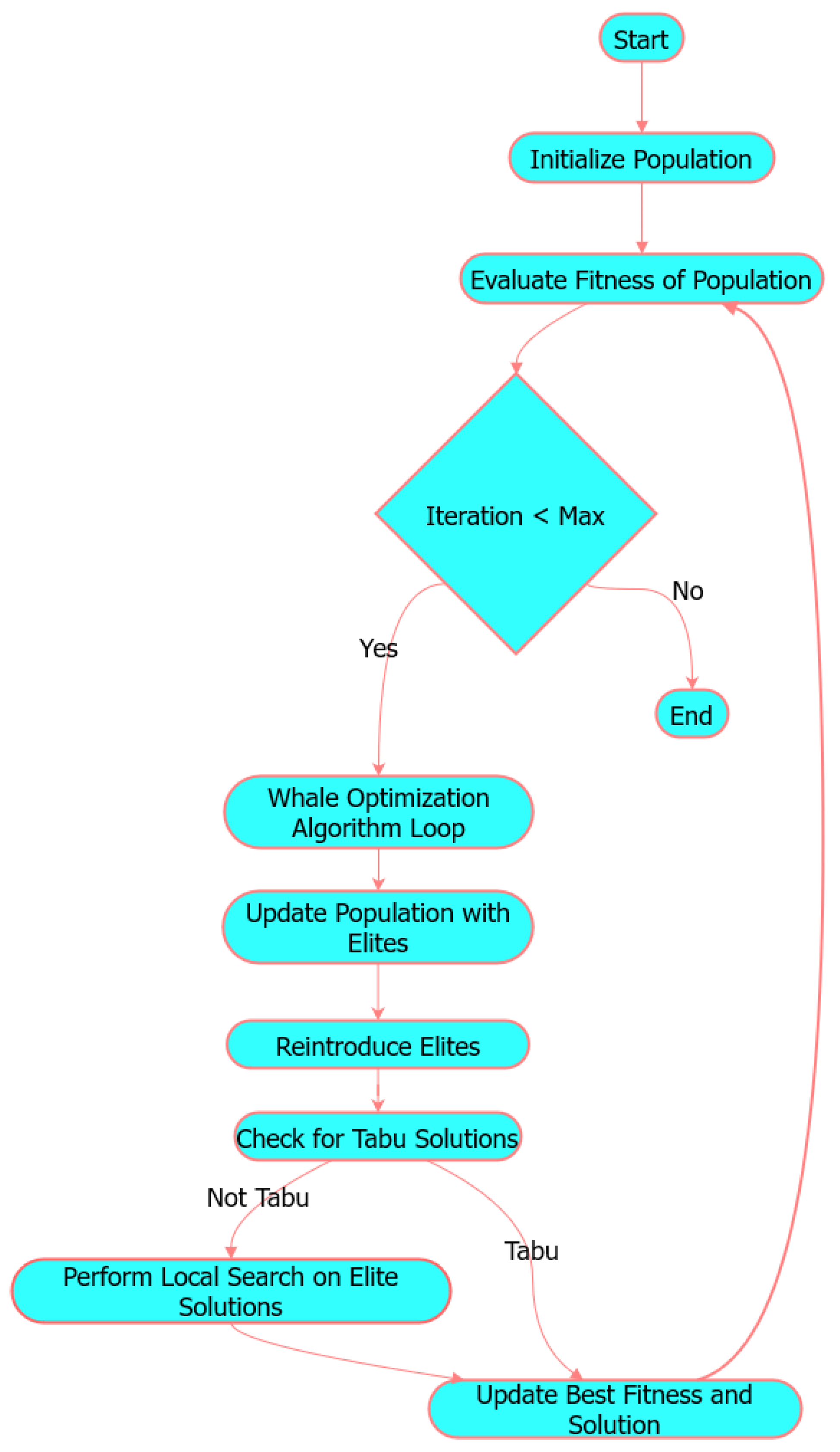
On the other hand, the local search strategy in LWOATS utilized the Nelder–Mead simplex method, addressing the fine-tuning of elite solutions identified from TS methods. This simply means that the algorithm would enhance its capability to closely explore the vicinity of the current best solution through the systematic adjustment of possible ones by simplex vertices, which probe different directions. This means that these areas are exploited to the maximum. The Nelder–Mead simplex further enhances the exploitation phase of the algorithm and contributes much to the general precision and effectiveness of the optimization process, with an assurance that the final solutions obtained are robust and near optimal. Figure 4 illustrates the flowchart diagram for LWOATS, while Algorithm 1 is the pseudocode for LWOATS.

Algorithm 1 LWOATS Optimization Algorithm

1: Initialize the whale population $X_i$, $i=1,2,\dots ,n$.   2: Evaluate the fitness value for the initial population   3: for each iteration do   4:      Update each agent’s position using WOA (Algorithm A1) enhanced by Levy flights   5:      Evaluate the fitness for new solutions   6:      Update elite solutions   7:      for each elite solution not in tabu list do   8:           Apply local search using Nelder–Mead   9:           Update best solution if improved   10:         Add new solution to tabu list   11:      end for   12:      Reintroduce elite solutions into the population   13: end for   14: Return the best solution and its fitness

3. Experimental Results and Discussion

LWOATS’s efficiency is evaluated through its application in 23 different benchmark functions as defined in the literature [65]. The first seven functions F1–F7 are unimodal high-dimensional functions and are presented in

Table A1. Unimodal benchmark functions.

Name	Function	Dim	Range	fmin
Sphere	$F_1\left(\mathbf{x}\right)={\sum }_{i=1}^d{x}_i^2$	30	$[-100,100]$	0
Schwefel2.22	$F_2\left(\mathbf{x}\right)={\sum }_{i=1}^d|x_i|+{\prod }_{i=1}^d\left|x_i\right|$	30	$[-10,10]$	0
Schwefel1.2	$F_3\left(\mathbf{x}\right)={\sum }_{j=1}^d{\left({\sum }_{i=1}^j{x}_i\right)}^2$	30	$[-100,100]$	0
Schwefel2.21	$F_4\left(\mathbf{x}\right)={max}_i\left\{\right|x_i|,1<i<d\}$	30	$[-100,100]$	0
Rosenbrock	$F_5\left(\mathbf{x}\right)={\sum }_{i=1}^{d-1}\left[100{(x_{i+1}-x_i^2)}^2+{(x_i-1)}^2\right]$	30	$[-30,30]$	0
Step	$F_6\left(\mathbf{x}\right)={\sum }_{i=1}^d{\left(\lfloor x_i+0.5\rfloor \right)}^2$	30	$[-100,100]$	0
Quartic	$F_7\left(\mathbf{x}\right)={\sum }_{i=1}^{d}i{x}_i^4+\mathrm{random}(0,1)$	30	$[-1.28,1.28]$	0

, while the next six functions in

Table A2. Multimodal benchmark functions.

Name	Function	Dim	Range	${\mathit{f}}_{\mathbf{min}}$
Zakharov	${\displaystyle F_8\left(\mathbf{x}\right)=\sum _{i=1}^d{x}_i^2+{\left(\sum _{i=1}^{d}0.5i{x}_i\right)}^2+{\left(\sum _{i=1}^{d}0.5i{x}_i\right)}^4}$	30	$[-5,10]$	0
Rastrigin	$F_9\left(\mathbf{x}\right)={\sum }_{i=1}^d\left(x_i^2-10cos\left(2\pi x_i\right)+10\right)$	30	$[-5.12,5.12]$	0
Ackley	$F_{10}\left(\mathbf{x}\right)=-20exp\left(-0.2\sqrt{{\displaystyle \frac{1}{d}}{\sum }_{i=1}^d{x}_i^2}\right)-exp\left({\displaystyle \frac{1}{d}}{\sum }_{i=1}^{d}cos\left(2\pi x_i\right)\right)+20+e$	30	$[-32,32]$	0
Griewank	$F_{11}\left(\mathbf{x}\right)={\displaystyle \frac{1}{4000}}{\sum }_{i=1}^d{x}_i^2-{\prod }_{i=1}^{d}cos\left({\displaystyle \frac{x_i}{\sqrt{i}}}\right)+1$	30	$[-600,600]$	0
Penalized 1	$\begin{array}{c}{F}_{12}\left(\mathbf{x}\right)=\\ {\displaystyle \frac{\pi }{d}}(10{sin}^2\left(\pi y_1\right)+{\sum }_{i=1}^{d-1}{\left(y_i-1\right)}^2\left[1+10{sin}^2\left(\pi y_{i+1}\right)\right]+{(y_d-1)}^2)+{\sum }_{i=1}^{d}U(x_i,10,100,4)\end{array}$
	where $y_i=1+{\displaystyle \frac{x_i+1}{4}}$, $U(x_i,a,k,m)=\left\{\begin{array}{cc}k{(x_i-a)}^m\hfill & \mathrm{if}{x}_i>a\hfill \\ 0\hfill & \mathrm{if}-a<x_i<a\hfill \\ k{(-x_i-a)}^m\hfill & \mathrm{if}{x}_i<-a\hfill \end{array}\right.$	30	$[-50,50]$	0
Penalized 2	$$\begin{array}{cc}\hfill F_{13}\left(\mathbf{x}\right)=& 0.1({sin}^2\left(3\pi x_1\right)+\sum _{i=1}^d{(x_i-1)}^2\left[1+{sin}^2(3\pi x_i+1)\right]\hfill \\ & \hspace{1em}+{(x_d-1)}^2\left[1+{sin}^2\left(2\pi x_d\right)\right])+\sum _{i=1}^{d}U(x_i,5,100,4)\hfill \end{array}$$	30	$[-50,50]$	0

F8–F13 are multimodal high-dimensional functions. Unimodal functions have only one global optimum, while multimodal functions have many local optima, and their complexity increases significantly as the dimensions increase, making them ideal candidate problems to test the exploration capabilities of the algorithm. All high-dimensional functions are tested in 30 dimensions to challenge the algorithms, while the boundaries and the global minimum for each one are represented in the corresponding table. All algorithms (LWOATS and comparisons) were terminated once they reached a fixed budget of $10.000$ objective function evaluations. Functions F14–F23 in

Table A3. Fixed-dimension multimodal benchmark functions.

Name	Function	Dim	Range	${\mathit{f}}_{\mathbf{min}}$
Shekel’s FoxHoles	$F_{14}\left(\mathbf{x}\right)={\left({\displaystyle \frac{1}{500}}+{\sum }_{i=1}^{25}{\displaystyle \frac{1}{i+{\sum }_{j=1}^2{(x_j-a_{ij})}^6}}\right)}^{-1}$	2	$[-65,65]$	1
Kowalik	$F_{15}\left(\mathbf{x}\right)={\sum }_{j=1}^{11}{\left(a_j-{\displaystyle \frac{x_1(b_j^2+b_j{x}_2)}{b_j^2+b_j{x}_3+x_4}}\right)}^2$	4	$[-5,5]$	0.00030
Six-Hump Camel	$F_{16}\left(\mathbf{x}\right)=4x_1^2-2.1x_1^4+{\displaystyle \frac{x_1^6}{3}}+x_1{x}_2-4x_2^2+4x_2^4$	2	$[-5,5]$	$-1.0316$
Drop wave	$F_{17}\left(\mathbf{x}\right)=-{\displaystyle \frac{1+cos\left(12\sqrt{x_1^2+x_2^2}\right)}{0.5(x_1^2+x_2^2)+2}}$	2	$[-5.12,5.12]$	−1
GoldStein Price	$\begin{array}{l}{F}_{18}\left(\mathbf{x}\right)=\left[1+{(x_1+x_2+1)}^2(19-14x_1+3x_1^2-14x_2+6x_1{x}_2+3x_2^2)\right]\times \\ \left[30+{(2x_1-3x_2)}^2(18-32x_1+12x_1^2+48x_2-36x_1{x}_2+27x_2^2)\right]\end{array}$	2	$[-5,5]$	3
Hartmann 3	$F_{19}\left(\mathbf{x}\right)=-{\sum }_{i=1}^4{c}_{i}exp\left(-{\sum }_{j=1}^3{a}_{ij}{(x_j-p_{ij})}^2\right)$	3	$[1,3]$	$-3.86$
Hartmann 6	$F_{20}\left(\mathbf{x}\right)=-{\sum }_{i=1}^4{c}_{i}exp\left(-{\sum }_{j=1}^6{a}_{ij}{(x_j-p_{ij})}^2\right)$	6	$[0,1]$	$-3.32$
Shekel 1	$F_{21}\left(\mathbf{x}\right)=-{\sum }_{i=1}^5{\left(\mathbf{x}-{\mathbf{a}}_i\right)}^{\top }\left(\mathbf{x}-{\mathbf{a}}_i\right)+c_i$	4	$[0,10]$	$-10.1532$
Shekel 2	$F_{22}\left(\mathbf{x}\right)=-{\sum }_{i=1}^7{\left(\mathbf{x}-{\mathbf{a}}_i\right)}^{\top }\left(\mathbf{x}-{\mathbf{a}}_i\right)+c_i$	4	$[0,10]$	$-10.4028$
Shekel 3	$F_{23}\left(\mathbf{x}\right)=-{\sum }_{i=1}^{10}{\left(\mathbf{x}-{\mathbf{a}}_i\right)}^{\top }\left(\mathbf{x}-{\mathbf{a}}_i\right)+c_i$	4	$[0,10]$	$-10.5363$

are fixed-dimension multimodal functions. The 2D representation of some of these functions is illustrated in Figure 5. All simulations were conducted on a laptop equipped with an Intel Core i7-1165G7 processor and 16 GB of RAM, utilizing Python 3.11.

3.1. Comparing LWOATS with Known Fundamental Algorithms

We compare LWOATS with known fundamental algorithms, including PSO, GWO, DE, and WOA. The parameters used in each algorithm are presented in

Table 1. Parameters of various optimization algorithms.

Algorithm	Parameters
WOA	$a\in [0,2]$, $p=\mathrm{rand}[0,1]$, $b=1$, $l\in [-1,1]$
DE	$pCR=0.2$, ${\beta }_{min}=0.2$, ${\beta }_{max}=0.8$
PSO	$w=0.7\to 0.4$, $C_1=2.0,C_2=1.0$
LWOATS	Same parameters with WOA, $\beta =1.5$ for Levy flights

. The Orthogonal Experimental Design (OED) method was followed to examine the algorithm’s various hyper-parameters simultaneously and fine-tune them to select the optimal ones, ensuring a fair comparison.

To guard against over-fitting our OED-derived settings to the full suite, we first ran the tuning on a small subset of six functions (two unimodal, two high-dimensional multimodal, and two fixed-dimension). We then applied exactly the same fixed hyper-parameters to all 23 functions (including those six) and, crucially, to the remaining 17 functions. LWOATS still outperforms or performs competitively in most cases, confirming that our parameters generalize beyond the calibration subset. To quantify each parameter’s impact, we conducted a full factorial design over four factors: population size: $[10,30,50,70,100]$, elite size ratio: $[0.1,0.2,0.3]$, tabu list ratio: $[0.1,0.2,0.3]$, and NM iterations: $[10,30,50,70,100]$. Each configuration ran under a fixed budget of 10.000 fitness evaluations on the training set of six functions, covering unimodal, high-D multimodal, and fixed-D multimodal landscapes, yielding 225 unique parameter combinations.

Results on Unimodal and Multimodal Functions

The OED analysis for LWOATS resulted in a population size of 10, a tabu size ratio and elite size ratio of 0.1, and a maximum number of Nelder–Mead iterations of 10 for all unimodal and multimodal functions. The results obtained from the ANOVA analysis are provided in

Table 2. ANOVA table for unimodal functions.

Source	sum_sq	df	f-Value	p-Value
C(pop_size)	7.3	4	14.7	$8.3\times {10}^{-12}$
C(elite_size_ratio)	5.4	2	21.9	$3.9\times {10}^{-10}$
C(local_search_max_iter)	0.7	4	1.5	$2.0\times {10}^{-10}$
C(tabu_size_ratio)	0.05	2	0.2	$8.1\times {10}^{-1}$

and 

Table 3. ANOVA table for high-dimensional multimodal functions.

Source	sum_sq	df	f-Value	p-Value
C(pop_size)	3.5	4	8.9	$4.2\times {10}^{-7}$
C(elite_size_ratio)	1.6	2	8.2	$3.0\times {10}^{-4}$
C(local_search_max_iter)	0.2	4	0.5	$7.2\times {10}^{-1}$
C(tabu_size_ratio)	0.07	2	0.4	$6.9\times {10}^{-1}$

. These results indicate that the population size and the elite size ratio have a significant impact on the algorithm’s performance since the p-values are smaller than 0.05. The maximum number of iterations for the Nelder–Mead operations and the tabu size ratio do not significantly affect the algorithm’s performance.

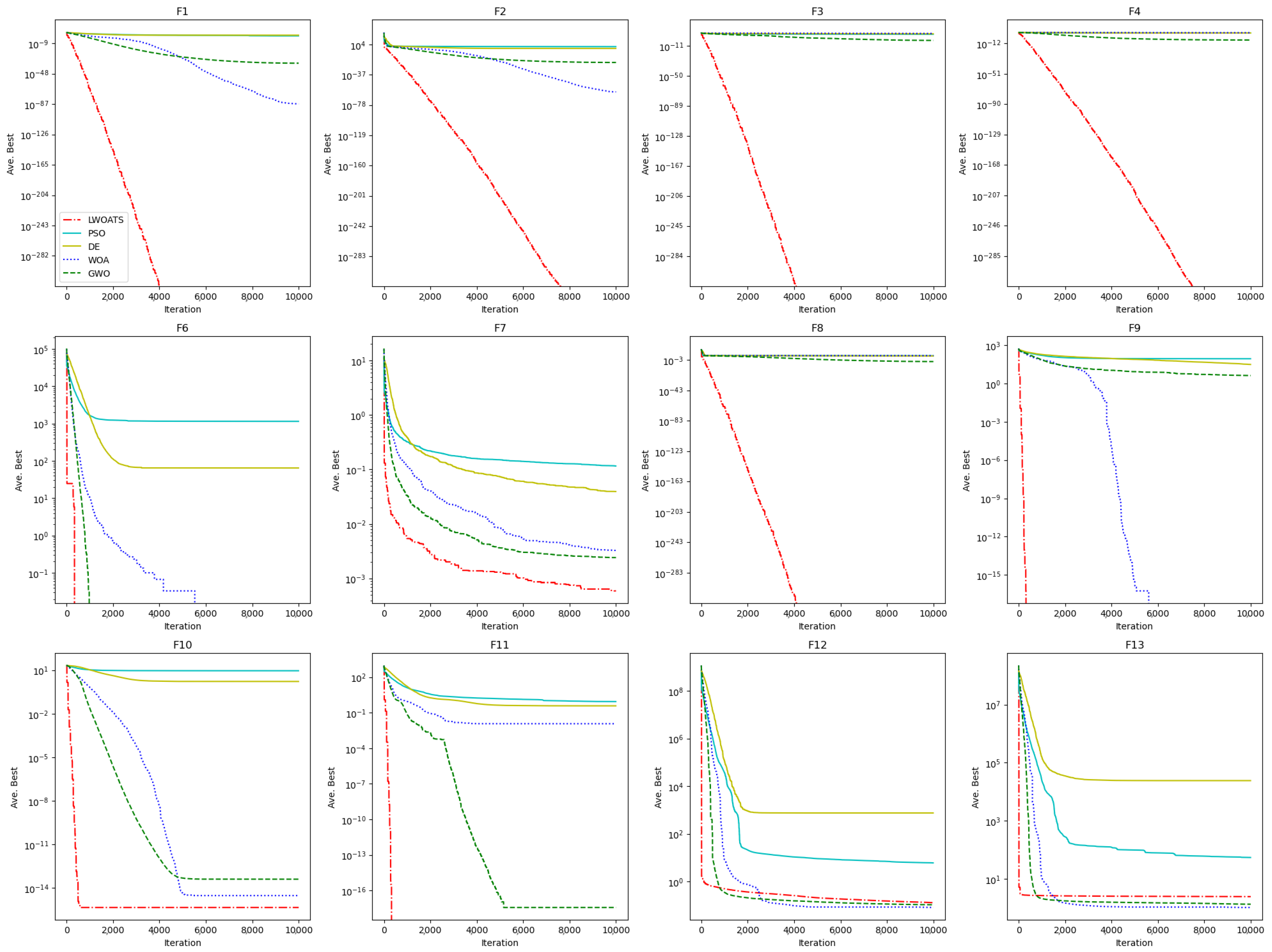
The results for the unimodal and high-dimensional multimodal functions (which have many local optima, so the good performance of the algorithm indicates its ability to explore the search space effectively and converge toward the best solution) are summarized in

Table A4. Performance of LWOATS and fundamental algorithms on unimodal functions.

Function	Result	Algorithms
		PSO	GWO	DE	WOA	LWOATS
F1	Best	$4.187\times {10}^{-5}$	$7.212\times {10}^{-38}$	$1.147\times {10}^{-8}$	$1.720\times {10}^{-111}$	0
	Worst	$3.486\times {10}^1$	$2.264\times {10}^{-34}$	$4.608\times {10}^2$	$5.472\times {10}^{-86}$	0
	Mean	$4.070\times {10}^0$	$3.453\times {10}^{-35}$	$3.269\times {10}^1$	$1.824\times {10}^{-87}$	0
	Std	$8.503\times {10}^0$	$5.405\times {10}^{-35}$	$9.357\times {10}^1$	$9.823\times {10}^{-87}$	0
F2	Best	$2.048\times {10}^{-1}$	$3.996\times {10}^{-22}$	$2.329\times {10}^{-9}$	$2.563\times {10}^{-73}$	0
	Worst	$3.213\times {10}^1$	$1.213\times {10}^{-20}$	$3.389\times {10}^{-1}$	$8.252\times {10}^{-60}$	0
	Mean	$1.132\times {10}^1$	$3.692\times {10}^{-21}$	$3.890\times {10}^{-2}$	$5.711\times {10}^{-61}$	0
	Std	$8.255\times {10}^0$	$2.851\times {10}^{-21}$	$8.650\times {10}^{-2}$	$1.995\times {10}^{-60}$	0
F3	Best	$4.139\times {10}^3$	$4.598\times {10}^0$	$2.896\times {10}^4$	$5.175\times {10}^4$	0
	Worst	$3.520\times {10}^4$	$8.145\times {10}^2$	$7.078\times {10}^4$	$2.440\times {10}^5$	0
	Mean	$1.534\times {10}^4$	$1.793\times {10}^2$	$4.521\times {10}^4$	$1.266\times {10}^5$	0
	Std	$7.756\times {10}^3$	$1.796\times {10}^2$	$8.836\times {10}^3$	$4.548\times {10}^4$	0
F4	Best	$2.082\times {10}^1$	$3.742\times {10}^{-1}$	$3.104\times {10}^1$	$2.716\times {10}^1$	0
	Worst	$4.297\times {10}^1$	$4.232\times {10}^0$	$5.492\times {10}^1$	$9.444\times {10}^1$	0
	Mean	$2.978\times {10}^1$	$1.142\times {10}^0$	$4.253\times {10}^1$	$7.091\times {10}^1$	0
	Std	$5.277\times {10}^0$	$7.594\times {10}^{-1}$	$5.817\times {10}^0$	$1.771\times {10}^1$	0
F5	Best	$2.889\times {10}^1$	$2.709\times {10}^1$	$3.606\times {10}^1$	$2.862\times {10}^1$	$2.606\times {10}^1$
	Worst	$2.326\times {10}^2$	$2.888\times {10}^1$	$2.242\times {10}^2$	$2.886\times {10}^1$	$2.886\times {10}^1$
	Mean	$7.815\times {10}^1$	$2.812\times {10}^1$	$1.173\times {10}^2$	$2.880\times {10}^1$	$2.746\times {10}^1$
	Std	$4.576\times {10}^1$	$6.648\times {10}^{-1}$	$5.397\times {10}^1$	$5.718\times {10}^{-2}$	$9.583\times {10}^{-1}$
F6	Best	$1.210\times {10}^2$	0	$1.300\times {10}^1$	0	0
	Worst	$4.998\times {10}^3$	$5.000\times {10}^0$	$3.150\times {10}^2$	$1.000\times {10}^0$	0
	Mean	$1.233\times {10}^3$	$1.067\times {10}^0$	$7.957\times {10}^1$	$3.333\times {10}^{-2}$	0
	Std	$1.143\times {10}^3$	$1.340\times {10}^0$	$7.068\times {10}^1$	$1.795\times {10}^{-1}$	0
F7	Best	$6.578\times {10}^{-2}$	$4.701\times {10}^{-3}$	$9.739\times {10}^{-2}$	$6.972\times {10}^{-4}$	$8.433\times {10}^{-6}$
	Worst	$3.329\times {10}^{-1}$	$4.240\times {10}^{-2}$	$4.540\times {10}^{-1}$	$1.137\times {10}^{-1}$	$1.270\times {10}^{-3}$
	Mean	$1.930\times {10}^{-1}$	$1.900\times {10}^{-2}$	$2.418\times {10}^{-1}$	$2.426\times {10}^{-2}$	$3.269\times {10}^{-4}$
	Std	$6.006\times {10}^{-2}$	$9.109\times {10}^{-3}$	$7.814\times {10}^{-2}$	$2.600\times {10}^{-2}$	$2.579\times {10}^{-4}$

and

Table A6. Performance of LWOATS and fundamental algorithms on high-dimensional multimodal functions.

Function	Result	Algorithms
		PSO	GWO	DE	WOA	LWOATS
F8	Best	$1.999\times {10}^2$	$1.267\times {10}^1$	$2.328\times {10}^2$	$3.137\times {10}^2$	0
	Worst	$9.596\times {10}^2$	$9.544\times {10}^1$	$5.676\times {10}^2$	$8.744\times {10}^2$	0
	Mean	$5.731\times {10}^2$	$3.896\times {10}^1$	$3.986\times {10}^2$	$5.397\times {10}^2$	0
	Std	$1.823\times {10}^2$	$1.950\times {10}^1$	$6.961\times {10}^1$	$1.258\times {10}^2$	0
F9	Best	$5.110\times {10}^1$	$8.777\times {10}^0$	$1.500\times {10}^2$	$5.8\times {10}^{-11}$	0
	Worst	$1.357\times {10}^2$	$6.809\times {10}^1$	$2.500\times {10}^2$	$2.400\times {10}^2$	0
	Mean	$9.699\times {10}^1$	$2.569\times {10}^1$	$2.200\times {10}^2$	$3.200\times {10}^1$	0
	Std	$2.181\times {10}^1$	$1.279\times {10}^1$	$1.800\times {10}^1$	$6.700\times {10}^1$	0
F10	Best	$5.466\times {10}^0$	$1.592\times {10}^{-3}$	$1.999\times {10}^0$	$7.173\times {10}^{-12}$	$4.441\times {10}^{-16}$
	Worst	$1.119\times {10}^1$	$1.340\times {10}^{-2}$	$7.582\times {10}^0$	$8.835\times {10}^{-8}$	$4.441\times {10}^{-16}$
	Mean	$9.738\times {10}^0$	$5.165\times {10}^{-3}$	$3.511\times {10}^0$	$1.231\times {10}^{-8}$	$4.441\times {10}^{-16}$
	Std	$2.240\times {10}^0$	$3.058\times {10}^{-3}$	$1.094\times {10}^0$	$2.286\times {10}^{-8}$	0
F11	Best	$1.174\times {10}^0$	$3.025\times {10}^{-4}$	$1.195\times {10}^0$	0	0
	Worst	$1.744\times {10}^1$	$1.253\times {10}^{-1}$	$3.753\times {10}^0$	$8.787\times {10}^{-1}$	0
	Mean	$4.170\times {10}^0$	$4.301\times {10}^{-2}$	$1.580\times {10}^0$	$5.143\times {10}^{-2}$	0
	Std	$3.872\times {10}^0$	$4.658\times {10}^{-2}$	$5.370\times {10}^{-1}$	$1.940\times {10}^{-1}$	0
F12	Best	$6.063\times {10}^0$	$1.030\times {10}^{-1}$	$2.864\times {10}^0$	$6.149\times {10}^{-2}$	$9.657\times {10}^{-7}$
	Worst	$5.997\times {10}^1$	$9.345\times {10}^{-1}$	$3.466\times {10}^4$	$9.739\times {10}^{-1}$	$3.104\times {10}^{-1}$
	Mean	$1.956\times {10}^1$	$4.375\times {10}^{-1}$	$1.978\times {10}^3$	$3.626\times {10}^{-1}$	$4.567\times {10}^{-2}$
	Std	$1.137\times {10}^1$	$2.444\times {10}^{-1}$	$7.076\times {10}^3$	$2.143\times {10}^{-1}$	$6.910\times {10}^{-2}$
F13	Best	$1.701\times {10}^1$	$1.416\times {10}^0$	$6.977\times {10}^0$	$1.026\times {10}^0$	$2.106\times {10}^{-2}$
	Worst	$1.271\times {10}^3$	$2.652\times {10}^0$	$1.212\times {10}^7$	$2.909\times {10}^0$	$2.984\times {10}^0$
	Mean	$1.552\times {10}^2$	$2.126\times {10}^0$	$4.044\times {10}^5$	$2.012\times {10}^0$	$2.141\times {10}^0$
	Std	$2.840\times {10}^2$	$3.118\times {10}^{-1}$	$2.175\times {10}^6$	$4.217\times {10}^{-1}$	$1.156\times {10}^0$

, respectively. LWOATS outperforms other algorithms in all cases. For most of the benchmark functions, it manages to reach the global minimum, i.e., 0 with pretty fast convergence. In particular, for functions F1, F3, F6, F8, F9, and F11, LWOATS needs 4000 or fewer evaluations to reach the global best, while for functions F2 and F4, less than 8000 evaluations are needed (Figure A1). LWOATS achieves good results in F7, but it poorly performs in F5. It is worth mentioning that our algorithm has the smallest standard deviation as calculated for all 30 independent runs.

To further evaluate the performance of the LWOATS against the PSO, DE, GWO, and WOAs on the unimodal functions, Wilcoxon signed-rank statistical tests were performed. In the Wilcoxon statistical test, the summarized ranks are calculated based on the difference between the best results as obtained by the tested algorithms for the i-th benchmark function. For each non-zero difference, the absolute value is calculated: $|D_i|=|X_i-Y_i|$, where $X_i$ is the result of LWOATS and $Y_i$ is the result of the compared algorithm for the i-th function. The absolute differences $|D_i|$ are then ranked in ascending order.

In our case, these values are calculated for the 30 independent runs on each benchmark problem. The sums of these positive and negative ranks are calculated based on the following equations:

$$R^{+}=\sum _{i:D_i>0}{R}_i\mathrm{and}{R}^{-}=\sum _{i:D_i<0}{R}_i,$$

where $R_i=\mathrm{rank}\left(\right|D_i\left|\right)$.

Table A5. Results of Wilcoxon statistical test for unimodal and high-dimensional multimodal functions for LWOATS and fundamental algorithms.

Comparison	${\mathit{R}}^{+}$	${\mathit{R}}^{-}$	+	−	=	Decision
LWOATS vs. DE	5871	153	13	0	0	+++++++++++++
LWOATS vs. GWO	3972	1118	8	2	3	++++−=++++==−
LWOATS vs. PSO	5657	388	13	0	0	+++++++++++++
LWOATS vs. WOA	3383	1248	7	2	4	++++−=++=+==−

summarizes the results obtained for the F1 to F13 benchmark functions for the 30 independent runs. The sum of positive ranks $R^{+}$ is always higher for LWOATS, indicating that it outperforms the other algorithms in most cases. More specifically, LWOATS significantly outperforms DE and PSO in all function comparisons, something that is also indicated by the low (less than 0.05) p-values in

Table A7. Wilcoxon’s p-values for each comparison of LWOATS and fundamental algorithms for the unimodal and high-dimensional multimodal functions.

Function	LWOATS vs. WOA	LWOATS vs. GWO	LWOATS vs. PSO	LWOATS vs. DE
F1	$1.8626\times {10}^{-9}$	$1.8626\times {10}^{-9}$	$1.8626\times {10}^{-9}$	$1.8626\times {10}^{-9}$
F2	$1.8626\times {10}^{-9}$	$1.8626\times {10}^{-9}$	$1.8626\times {10}^{-9}$	$1.8626\times {10}^{-9}$
F3	$1.8626\times {10}^{-9}$	$1.8626\times {10}^{-9}$	$1.8626\times {10}^{-9}$	$1.8626\times {10}^{-9}$
F4	$1.8626\times {10}^{-9}$	$1.8626\times {10}^{-9}$	$1.8626\times {10}^{-9}$	$1.8626\times {10}^{-9}$
F5	$5.1446\times {10}^{-6}$	$2.6077\times {10}^{-8}$	$8.7182\times {10}^{-4}$	$1.8626\times {10}^{-9}$
F6	$1.0000\times {10}^0$	$1.0000\times {10}^0$	$1.8626\times {10}^{-9}$	$4.6595\times {10}^{-6}$
F7	$8.7182\times {10}^{-4}$	$3.7253\times {10}^{-9}$	$1.8626\times {10}^{-9}$	$1.8626\times {10}^{-9}$
F8	$1.8626\times {10}^{-9}$	$1.8626\times {10}^{-9}$	$1.8626\times {10}^{-9}$	$1.8626\times {10}^{-9}$
F9	$1.0000\times {10}^0$	$1.7410\times {10}^{-5}$	$1.8626\times {10}^{-9}$	$1.8626\times {10}^{-9}$
F10	$2.9009\times {10}^{-5}$	$1.8626\times {10}^{-9}$	$1.8626\times {10}^{-9}$	$1.8626\times {10}^{-9}$
F11	$1.6452\times {10}^{-1}$	$3.3371\times {10}^{-1}$	$1.8626\times {10}^{-9}$	$1.8626\times {10}^{-9}$
F12	$2.9884\times {10}^{-1}$	$6.8505\times {10}^{-1}$	$1.8626\times {10}^{-9}$	$1.2184\times {10}^{-5}$
F13	$1.0245\times {10}^{-7}$	$5.7183\times {10}^{-7}$	$1.8626\times {10}^{-9}$	$1.4538\times {10}^{-2}$

. LWOATS also outperforms or shows a competitive performance over GWO and WOA in most cases. GWO and WOA perform better only in F5 and F13, while there are three functions (F6, F11, and F12) where LWOATS has a similar performance to GWO and four functions (F6, F9, F11, and F12) where LWOATS has a similar performance to WOA. The symbols ‘+’, ‘−’, and ‘=’ are used in this table to indicate which algorithm performs better, worse, or if they perform similarly, respectively. These symbols are also aligned with the p-values obtained by the test, indicating significant differences in the results (if ‘+’ or ‘−’) or not (if ‘=’). The convergence curves for some of the unimodal and high-dimensional multimodal benchmark functions are presented in Figure A1.

Finally, LWOATS results on the fixed-dimension multimodal functions (Table A3) are presented in

Table A9. Performance of LWOATS and fundamental algorithms on fixed-dimension multimodal functions.

Function	Result	Algorithms
		PSO	GWO	DE	WOA	LWOATS
F14	Best	$9.980\times {10}^{-1}$	$9.980\times {10}^{-1}$	$9.980\times {10}^{-1}$	$9.980\times {10}^{-1}$	$9.980\times {10}^{-1}$
	Worst	$1.076\times {10}^1$	$1.644\times {10}^1$	$1.076\times {10}^1$	$1.644\times {10}^1$	$1.267\times {10}^1$
	Mean	$2.675\times {10}^0$	$7.535\times {10}^0$	$2.482\times {10}^0$	$5.886\times {10}^0$	$1.138\times {10}^1$
	Std	$2.320\times {10}^0$	$5.028\times {10}^0$	$2.479\times {10}^0$	$4.798\times {10}^0$	$3.334\times {10}^0$
F15	Best	$3.575\times {10}^{-4}$	$3.121\times {10}^{-4}$	$7.155\times {10}^{-4}$	$3.127\times {10}^{-4}$	$3.076\times {10}^{-4}$
	Worst	$2.036\times {10}^{-2}$	$2.100\times {10}^{-2}$	$2.036\times {10}^{-2}$	$2.255\times {10}^{-2}$	$1.235\times {10}^{-3}$
	Mean	$4.102\times {10}^{-3}$	$4.650\times {10}^{-3}$	$3.225\times {10}^{-3}$	$2.575\times {10}^{-3}$	$4.795\times {10}^{-4}$
	Std	$6.764\times {10}^{-3}$	$7.964\times {10}^{-3}$	$5.011\times {10}^{-3}$	$4.632\times {10}^{-3}$	$2.531\times {10}^{-4}$
F16	Best	$-1.0316\times {10}^0$	$-1.0316\times {10}^0$	$-1.0316\times {10}^0$	$-1.0316\times {10}^0$	$-1.0316\times {10}^0$
	Worst	$-1.0316\times {10}^0$	$-1.0316\times {10}^0$	$-1.0315\times {10}^0$	$-1.0315\times {10}^0$	$-1.0316\times {10}^0$
	Mean	$-1.0316\times {10}^0$	$-1.0316\times {10}^0$	$-1.0316\times {10}^0$	$-1.0316\times {10}^0$	$-1.0316\times {10}^0$
	Std	$2.183\times {10}^{-16}$	$6.482\times {10}^{-7}$	$1.532\times {10}^{-5}$	$1.268\times {10}^{-5}$	$3.888\times {10}^{-8}$
F17	Best	$-1.0\times {10}^0$	$-1.0\times {10}^0$	$-1.0\times {10}^0$	$-1.0\times {10}^0$	$-1.0\times {10}^0$
	Worst	$-9.362\times {10}^{-1}$	$-9.362\times {10}^{-1}$	$-9.362\times {10}^{-1}$	$-9.362\times {10}^{-1}$	$-1.0\times {10}^0$
	Mean	$-9.863\times {10}^{-1}$	$-9.575\times {10}^{-1}$	$-9.785\times {10}^{-1}$	$-9.724\times {10}^{-1}$	$-1.0\times {10}^0$
	Std	$2.552\times {10}^{-2}$	$3.005\times {10}^{-2}$	$2.992\times {10}^{-2}$	$3.159\times {10}^{-2}$	0
F18	Best	$3.0\times {10}^0$	$3.0\times {10}^0$	$3.0\times {10}^0$	$3.0\times {10}^0$	$3.0\times {10}^0$
	Worst	$8.4\times {10}^1$	$8.4\times {10}^1$	$3.0\times {10}^0$	$3.147\times {10}^1$	$3.0\times {10}^0$
	Mean	$5.7\times {10}^0$	$9.3\times {10}^0$	$3.0\times {10}^0$	$8.548\times {10}^0$	$3.0\times {10}^0$
	Std	$1.454\times {10}^1$	$2.054\times {10}^1$	$9.735\times {10}^{-10}$	$1.106\times {10}^1$	$9.574\times {10}^{-6}$
F19	Best	$-3.863\times {10}^0$	$-3.863\times {10}^0$	$-3.863\times {10}^0$	$-3.863\times {10}^0$	$-3.863\times {10}^0$
	Worst	$-3.090\times {10}^0$	$-3.853\times {10}^0$	$-3.090\times {10}^0$	$-3.582\times {10}^0$	$-3.863\times {10}^0$
	Mean	$-3.837\times {10}^0$	$-3.860\times {10}^0$	$-3.837\times {10}^0$	$-3.790\times {10}^0$	$-3.863\times {10}^0$
	Std	$1.388\times {10}^{-1}$	$2.904\times {10}^{-3}$	$1.388\times {10}^{-1}$	$9.887\times {10}^{-2}$	$2.786\times {10}^{-5}$
F20	Best	$-3.322\times {10}^0$	$-3.322\times {10}^0$	$-3.322\times {10}^0$	$-3.313\times {10}^0$	$-3.322\times {10}^0$
	Worst	$-2.840\times {10}^0$	$-3.102\times {10}^0$	$-3.138\times {10}^0$	$-1.588\times {10}^0$	$-3.199\times {10}^0$
	Mean	$-3.268\times {10}^0$	$-3.266\times {10}^0$	$-3.294\times {10}^0$	$-3.007\times {10}^0$	$-3.286\times {10}^0$
	Std	$1.034\times {10}^{-1}$	$8.164\times {10}^{-2}$	$4.806\times {10}^{-2}$	$3.134\times {10}^{-1}$	$5.467\times {10}^{-2}$
F21	Best	$-1.01532\times {10}^1$	$-1.0152\times {10}^1$	$-1.0151\times {10}^1$	$-1.0151\times {10}^1$	$-1.01532\times {10}^1$
	Worst	$-2.630\times {10}^0$	$-5.055\times {10}^0$	$-2.617\times {10}^0$	$-2.626\times {10}^0$	$-1.01532\times {10}^1$
	Mean	$-6.726\times {10}^0$	$-9.813\times {10}^0$	$-6.376\times {10}^0$	$-8.235\times {10}^0$	$-1.01532\times {10}^1$
	Std	$3.324\times {10}^0$	$1.265\times {10}^0$	$3.394\times {10}^0$	$2.654\times {10}^0$	$1.17\times {10}^{-8}$
F22	Best	$-1.04029\times {10}^1$	$-1.04027\times {10}^1$	$-1.04012\times {10}^1$	$-1.04024\times {10}^1$	$-1.04029\times {10}^1$
	Worst	$-2.765\times {10}^0$	$-1.0397\times {10}^1$	$-2.749\times {10}^0$	$-1.8356\times {10}^0$	$-1.04029\times {10}^1$
	Mean	$-8.316\times {10}^0$	$-1.040\times {10}^1$	$-7.1236\times {10}^0$	$-7.3941\times {10}^0$	$-1.04029\times {10}^1$
	Std	$2.983\times {10}^0$	$1.08\times {10}^{-3}$	$3.511\times {10}^0$	$3.051\times {10}^0$	$1.01\times {10}^{-8}$
F23	Best	$-1.05364\times {10}^1$	$-1.05362\times {10}^1$	$-1.05314\times {10}^1$	$-1.05357\times {10}^1$	$-1.05364\times {10}^1$
	Worst	$-2.427\times {10}^0$	$-1.05312\times {10}^1$	$-2.412\times {10}^0$	$-2.421\times {10}^0$	$-1.05364\times {10}^1$
	Mean	$-8.133\times {10}^0$	$-1.05343\times {10}^1$	$-8.276\times {10}^0$	$-6.585\times {10}^0$	$-1.05364\times {10}^1$
	Std	$3.447\times {10}^0$	$1.196\times {10}^{-3}$	$3.445\times {10}^0$	$3.020\times {10}^0$	$1.20\times {10}^{-8}$

. LWOATS demonstrates a competitive performance, yielding optimal solutions across the majority of tested scenarios. While its performance is suboptimal in F14, where it gets outperformed by the rest of the algorithms, it successfully identifies the global minimum in most of the other complex benchmark functions. In particular, LWOATS outperforms DE and PSO over the benchmark functions F15, F17, F20, F21, F22, and F23 or shows a competitive performance in the case of F16, F18, and F19 based on Wilcoxon’s test results, which are presented in

Table A8. Results of Wilcoxon statistical test for fixed-dimension multimodal functions for LWOATS and fundamental algorithms.

Comparison	${\mathit{R}}^{+}$	${\mathit{R}}^{-}$	+	−	=	Decision
LWOATS vs. DE	2385	870	6	1	3	−+=+==++++
LWOATS vs. GWO	3811	539	9	1	0	−++++++++
LWOATS vs. PSO	2007	1237	6	1	3	−+=+==++++
LWOATS vs. WOA	3936	543	9	1	0	−+++++++++

. Additionally, the low p-values (less than 0.05) in

Table A10. Wilcoxon’s p-values for each comparison of LWOATS and fundamental algorithms for the fixed-dimension multimodal functions.

Function	LWOATS vs. WOA	LWOATS vs. GWO	LWOATS vs. PSO	LWOATS vs. DE
F14	$3.128\times {10}^{-4}$	$6.640\times {10}^{-3}$	$3.681\times {10}^{-6}$	$1.863\times {10}^{-9}$
F15	$1.684\times {10}^{-6}$	$1.192\times {10}^{-6}$	$1.192\times {10}^{-6}$	$8.010\times {10}^{-8}$
F16	$9.313\times {10}^{-9}$	$3.725\times {10}^{-9}$	$1.000\times {10}^0$	$1.000\times {10}^0$
F17	$6.296\times {10}^{-4}$	$1.510\times {10}^{-2}$	$2.896\times {10}^{-6}$	$1.863\times {10}^{-9}$
F18	$1.863\times {10}^{-9}$	$1.863\times {10}^{-9}$	$1.000\times {10}^0$	$1.000\times {10}^0$
F19	$1.863\times {10}^{-9}$	$1.863\times {10}^{-9}$	$1.000\times {10}^0$	$1.000\times {10}^0$
F20	$2.622\times {10}^{-3}$	$2.622\times {10}^{-2}$	$2.774\times {10}^{-2}$	$5.382\times {10}^{-3}$
F21	$1.863\times {10}^{-9}$	$1.863\times {10}^{-9}$	$1.863\times {10}^{-9}$	$9.220\times {10}^{-6}$
F22	$1.863\times {10}^{-9}$	$1.863\times {10}^{-9}$	$6.554\times {10}^{-1}$	$1.863\times {10}^{-9}$
F23	$9.983\times {10}^{-7}$	$2.762\times {10}^{-6}$	$2.206\times {10}^{-1}$	$3.790\times {10}^{-6}$

indicate that the LWOATS performance is significantly better. Our approach achieves even better results when comparing it with WOA and GWO by outperforming these algorithms in 9 out of 10 cases. Also, the fact that LWOATS performs better in complex cases such as Shekel’s functions (F21–F23), where many metaheuristic approaches in the literature tend to underperform, underscores LWOATS’ capability to navigate multimodal landscapes and escape local minima effectively due to the incorporated Levy flights and memory elements.

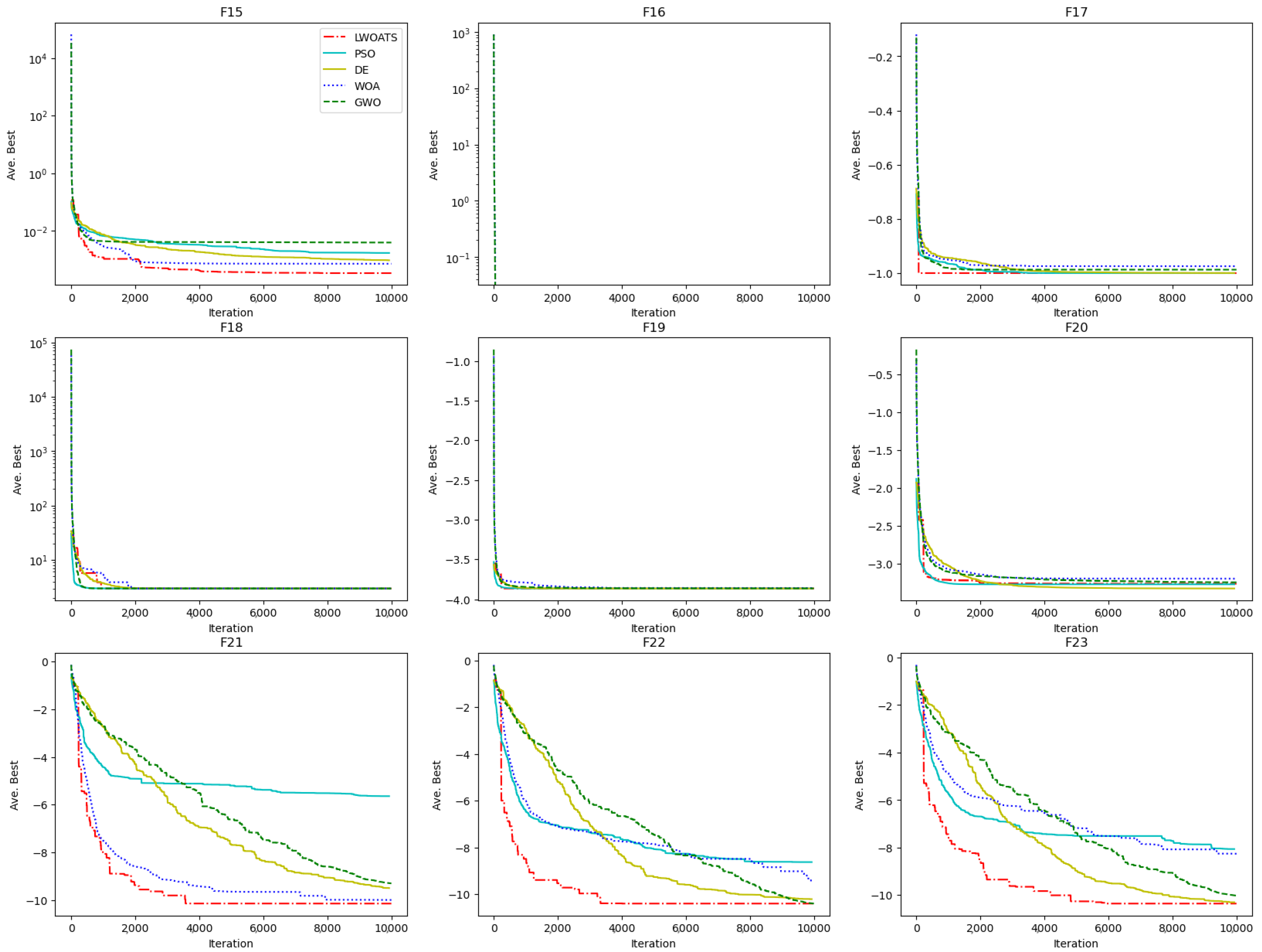
Overall, LWOATS demonstrates a superior performance compared to DE in 19 out of 23 benchmark functions, shows competitive results in 3, and underperforms in just 1. When compared to GWO, LWOATS outperforms in 17 out of 23 problems, delivers a competitive performance in 3, and performs worse in 3. Against PSO, LWOATS shows the same performance as its comparison with DE. Lastly, when compared to WOA, LWOATS performs better in 16 out of 23 problems, is competitive in 4, and performs worse in 3. The convergence curves for the fixed-dimension multimodal benchmark functions are presented in Figure A2.

3.2. Comparing LWOATS with Advanced DE Variations

LWOATS was tested against advanced DE variants such as SaDE, JADE, jSO, and iL-SHADE to assess its performance against well-established and highly competitive algorithms (winners of CEC competitions) in the field. The optimization parameters remain the same as obtained by the OED analysis, while for the DE variants, we used the default parameters from the PyADE [66] library as they are summarized in

Table 4. Default parameters for differential evolution variants in PyADE.

Algorithm	Parameter	Default Value
SaDE	Crossover Probability ($CR$), Mutation Factor (F)	$CR=0.9$, $F=0.5$
JADE	Proportion of best solutions (p), Parameter control (c)	$p=0.1$, $c=0.1$
iL-SHADE	Memory Size (H)	$H=5$
jSO	Memory Size (H)	$H=5$

. Each test was executed for a population size of 10 and 10,000 max evaluations. The results for the unimodal functions (F1–F7) are presented in

Table A11. Performance of LWOATS and advanced DE variants on unimodal functions.

Function	Result	Algorithms
		SaDE	JADE	iL-SHADE	jSO	LWOATS
F1	Best	$7.946\times {10}^{-1}$	$5.456\times {10}^{-1}$	$9.100\times {10}^{-5}$	$2.920\times {10}^{-4}$	0
	Worst	$1.456\times {10}^0$	$9.944\times {10}^{-1}$	$6.830\times {10}^{-4}$	$1.557\times {10}^{-3}$	0
	Mean	$1.110\times {10}^0$	$7.246\times {10}^{-1}$	$3.660\times {10}^{-4}$	$7.880\times {10}^{-4}$	0
	Std	$1.686\times {10}^{-1}$	$1.039\times {10}^{-1}$	$1.681\times {10}^{-4}$	$3.220\times {10}^{-4}$	0
F2	Best	$3.516\times {10}^0$	$3.291\times {10}^0$	$3.425\times {10}^{-2}$	$4.825\times {10}^{-2}$	0
	Worst	$5.212\times {10}^0$	$4.312\times {10}^0$	$8.068\times {10}^{-2}$	$1.338\times {10}^{-1}$	0
	Mean	$4.551\times {10}^0$	$3.719\times {10}^0$	$5.210\times {10}^{-2}$	$8.629\times {10}^{-2}$	0
	Std	$3.590\times {10}^{-1}$	$2.766\times {10}^{-1}$	$1.017\times {10}^{-2}$	$2.109\times {10}^{-2}$	0
F3	Best	$4.063\times {10}^0$	$4.662\times {10}^0$	$9.390\times {10}^{-3}$	$4.435\times {10}^{-2}$	0
	Worst	$3.520\times {10}^4$	$9.927\times {10}^0$	$9.127\times {10}^{-2}$	$1.479\times {10}^{-1}$	0
	Mean	$6.012\times {10}^0$	$6.763\times {10}^0$	$3.894\times {10}^{-2}$	$9.822\times {10}^{-2}$	0
	Std	$7.756\times {10}^3$	$1.190\times {10}^0$	$1.730\times {10}^{-2}$	$2.886\times {10}^{-2}$	0
F4	Best	$4.622\times {10}^{-1}$	$4.491\times {10}^{-1}$	$2.040\times {10}^{-2}$	$2.866\times {10}^{-2}$	0
	Worst	$7.767\times {10}^{-1}$	$6.932\times {10}^{-1}$	$5.995\times {10}^{-2}$	$9.694\times {10}^{-2}$	0
	Mean	$6.494\times {10}^{-1}$	$6.046\times {10}^{-1}$	$3.865\times {10}^{-2}$	$5.665\times {10}^{-2}$	0
	Std	$5.574\times {10}^{-2}$	$5.095\times {10}^{-2}$	$8.758\times {10}^{-3}$	$1.613\times {10}^{-2}$	0
F5	Best	$1.361\times {10}^2$	$9.713\times {10}^1$	$2.673\times {10}^1$	$2.784\times {10}^1$	$2.606\times {10}^1$
	Worst	$2.156\times {10}^2$	$1.611\times {10}^2$	$2.956\times {10}^1$	$2.939\times {10}^1$	$2.886\times {10}^1$
	Mean	$1.800\times {10}^2$	$1.297\times {10}^2$	$2.810\times {10}^1$	$2.845\times {10}^1$	$2.746\times {10}^1$
	Std	$2.128\times {10}^1$	$1.614\times {10}^1$	$4.652\times {10}^{-1}$	$3.299\times {10}^{-1}$	$9.583\times {10}^{-1}$
F6	Best	0	0	0	0	0
	Worst	$1.0\times {10}^0$	$1.0\times {10}^0$	0	0	0
	Mean	$3.667\times {10}^{-1}$	$3.333\times {10}^{-2}$	0	0	0
	Std	$4.819\times {10}^{-1}$	$1.795\times {10}^{-1}$	0	0	0
F7	Best	$1.284\times {10}^{-1}$	$1.148\times {10}^{-1}$	$3.418\times {10}^{-3}$	$4.695\times {10}^{-3}$	$8.433\times {10}^{-6}$
	Worst	$4.334\times {10}^{-1}$	$2.420\times {10}^{-1}$	$2.337\times {10}^{-2}$	$2.212\times {10}^{-2}$	$1.270\times {10}^{-3}$
	Mean	$2.254\times {10}^{-1}$	$1.723\times {10}^{-1}$	$1.038\times {10}^{-2}$	$1.372\times {10}^{-2}$	$3.269\times {10}^{-4}$
	Std	$6.688\times {10}^{-2}$	$2.867\times {10}^{-2}$	$4.659\times {10}^{-3}$	$4.875\times {10}^{-3}$	$2.579\times {10}^{-4}$

, while the results for the high-dimensional multimodal functions (F8–F13) are summarized in

Table A13. Performance comparison of LWOATS with advanced DE variants on high-dimensional multimodal functions.

Function	Result	Algorithms
		SaDE	JADE	iL-SHADE	jSO	LWOATS
F8	Best	$5.894\times {10}^0$	$6.080\times {10}^0$	$1.526\times {10}^{-2}$	$1.754\times {10}^{-1}$	0
	Worst	$1.283\times {10}^1$	$1.474\times {10}^1$	$1.588\times {10}^{-1}$	$4.632\times {10}^{-1}$	0
	Mean	$9.931\times {10}^0$	$1.139\times {10}^1$	$9.499\times {10}^{-2}$	$2.884\times {10}^{-1}$	0
	Std	$1.565\times {10}^0$	$2.017\times {10}^1$	$3.314\times {10}^{-2}$	$6.047\times {10}^{-2}$	0
F9	Best	$1.101\times {10}^2$	$1.356\times {10}^2$	$1.029\times {10}^2$	$1.321\times {10}^2$	0
	Worst	$1.640\times {10}^2$	$1.771\times {10}^2$	$1.472\times {10}^2$	$1.728\times {10}^2$	0
	Mean	$1.359\times {10}^2$	$1.580\times {10}^2$	$1.259\times {10}^2$	$1.541\times {10}^2$	0
	Std	$1.018\times {10}^2$	$1.139\times {10}^1$	$1.197\times {10}^1$	$1.021\times {10}^1$	0
F10	Best	$1.709\times {10}^0$	$1.456\times {10}^0$	$6.855\times {10}^{-3}$	$1.272\times {10}^{-2}$	$4.441\times {10}^{-16}$
	Worst	$2.194\times {10}^0$	$1.941\times {10}^0$	$4.138\times {10}^{-2}$	$5.115\times {10}^{-2}$	$4.441\times {10}^{-16}$
	Mean	$1.956\times {10}^0$	$1.714\times {10}^0$	$1.634\times {10}^{-2}$	$2.475\times {10}^{-2}$	$4.441\times {10}^{-16}$
	Std	$1.326\times {10}^{-1}$	$1.109\times {10}^{-1}$	$6.525\times {10}^{-3}$	$8.837\times {10}^{-3}$	0
F11	Best	$2.683\times {10}^{-2}$	$2.296\times {10}^{-2}$	$5.000\times {10}^{-6}$	$1.400\times {10}^{-5}$	0
	Worst	$7.833\times {10}^{-2}$	$4.879\times {10}^{-2}$	$5.300\times {10}^{-5}$	$7.800\times {10}^{-5}$	0
	Mean	$5.212\times {10}^{-2}$	$3.897\times {10}^{-2}$	$2.300\times {10}^{-5}$	$3.900\times {10}^{-5}$	0
	Std	$1.096\times {10}^{-2}$	$5.019\times {10}^{-3}$	$1.258\times {10}^{-5}$	$1.668\times {10}^{-5}$	0
F12	Best	$2.766\times {10}^{-2}$	$1.542\times {10}^{-2}$	$1.000\times {10}^{-5}$	$1.500\times {10}^{-5}$	$9.657\times {10}^{-7}$
	Worst	$6.974\times {10}^{-2}$	$3.586\times {10}^{-2}$	$1.230\times {10}^{-4}$	$2.510\times {10}^{-4}$	$3.104\times {10}^{-1}$
	Mean	$3.880\times {10}^{-2}$	$2.513\times {10}^{-2}$	$4.700\times {10}^{-5}$	$9.100\times {10}^{-5}$	$4.567\times {10}^{-2}$
	Std	$8.130\times {10}^{-3}$	$4.829\times {10}^{-3}$	$2.727\times {10}^{-5}$	$5.722\times {10}^{-5}$	$6.910\times {10}^{-2}$
F13	Best	$2.778\times {10}^{-1}$	$2.109\times {10}^{-1}$	$2.360\times {10}^{-4}$	$3.700\times {10}^{-4}$	$2.106\times {10}^{-2}$
	Worst	$5.486\times {10}^{-1}$	$3.426\times {10}^{-1}$	$3.972\times {10}^{-3}$	$3.451\times {10}^{-3}$	$2.984\times {10}^0$
	Mean	$4.234\times {10}^{-1}$	$2.806\times {10}^{-1}$	$9.440\times {10}^{-4}$	$1.270\times {10}^{-3}$	$2.141\times {10}^0$
	Std	$6.193\times {10}^{-2}$	$2.891\times {10}^{-2}$	$7.279\times {10}^{-4}$	$7.312\times {10}^{-4}$	$1.156\times {10}^0$

. Wilcoxon’s test results for the unimodal and high-dimensional multimodal functions are presented in

Table A16. Results of Wilcoxon statistical test for fixed-dimension multimodal functions for LWOATS and advanced DE algorithms.

Comparison	${\mathit{R}}^{+}$	${\mathit{R}}^{-}$	+	−	=	Decision
LWOATS vs. SaDE	4981	874	12	1	0	+++++++++++−−
LWOATS vs. JADE	4684	926	11	1	1	+++++=+++++−−
LWOATS vs. iL-SHADE	4216	1364	9	3	1	++++−=+++++−−
LWOATS vs. jSO	4324	1256	9	3	1	++++−=+++++−−

.

These algorithms perform better than DE in unimodal and high-dimensional multimodal functions. However, LWOATS can still outperform or even be competitive against them in most scenarios. SaDE and JADE achieve better results than LWOATS only in the F13 benchmark function, while JADE has a similar performance to LWOATS only in the F6 function. iL-SHADE and jSO outperform LWOATS in F5, F12, and F13 benchmark functions and have similar behavior only in F6. The low p-values in

Table A14. Wilcoxon’s p-values for each comparison of LWOATS and advanced DE variants for the unimodal and high-dimensional multimodal functions.

Function	LWOATS vs. SaDE	LWOATS vs. JADE	LWOATS vs. iL-SHADE	LWOATS vs. jSO
F1	$1.863\times {10}^{-9}$	$1.863\times {10}^{-9}$	$1.863\times {10}^{-9}$	$1.863\times {10}^{-9}$
F2	$1.863\times {10}^{-9}$	$1.863\times {10}^{-9}$	$1.863\times {10}^{-9}$	$1.863\times {10}^{-9}$
F3	$1.863\times {10}^{-9}$	$1.863\times {10}^{-9}$	$1.863\times {10}^{-9}$	$1.863\times {10}^{-9}$
F4	$1.863\times {10}^{-9}$	$1.863\times {10}^{-9}$	$1.863\times {10}^{-9}$	$1.863\times {10}^{-9}$
F5	$1.863\times {10}^{-9}$	$1.863\times {10}^{-9}$	$4.422\times {10}^{-6}$	$5.492\times {10}^{-2}$
F6	$9.512\times {10}^{-4}$	$3.337\times {10}^{-1}$	$1.000\times {10}^0$	$1.000\times {10}^0$
F7	$1.863\times {10}^{-9}$	$1.863\times {10}^{-9}$	$1.863\times {10}^{-9}$	$1.863\times {10}^{-9}$
F8	$1.863\times {10}^{-9}$	$1.863\times {10}^{-9}$	$1.863\times {10}^{-9}$	$1.863\times {10}^{-9}$
F9	$1.863\times {10}^{-9}$	$1.863\times {10}^{-9}$	$1.863\times {10}^{-9}$	$1.863\times {10}^{-9}$
F10	$1.863\times {10}^{-9}$	$1.863\times {10}^{-9}$	$1.863\times {10}^{-9}$	$1.863\times {10}^{-9}$
F11	$1.863\times {10}^{-9}$	$1.863\times {10}^{-9}$	$1.863\times {10}^{-9}$	$1.863\times {10}^{-9}$
F12	$1.106\times {10}^{-4}$	$1.304\times {10}^{-8}$	$1.863\times {10}^{-9}$	$1.863\times {10}^{-9}$
F13	$1.863\times {10}^{-9}$	$1.863\times {10}^{-9}$	$1.863\times {10}^{-9}$	$1.863\times {10}^{-9}$

suggest a significant difference in the performance of the algorithms across most cases.

In the case of fixed-dimension multimodal functions, LWOATS consistently outperforms the advanced DE variants in most cases, particularly in functions F14 to F17 and F21 to F23. However, the other algorithms show a better performance in functions F18, F19, and F20, while JADE and jSO show a similar performance to LWOATS in F17. The Wilcoxon’s test results for this analysis are presented in

Table A17. Results of Wilcoxon statistical test for fixed-dimension multimodal functions for LWOATS and advanced DE variants.

Comparison	${\mathit{R}}^{+}$	${\mathit{R}}^{-}$	+	−	=	Decision
LWOATS vs. SaDE	2875	1544	7	3	0	++++−−−+++
LWOATS vs. JADE	2680	1505	6	3	1	+++=−−−+++
LWOATS vs. iL-SHADE	2707	1565	6	3	1	+++=−−−+++
LWOATS vs. jSO	2582	1603	6	3	1	+++=−−−+++

, and the p-values for each algorithm comparison are included in

Table A18. Wilcoxon’s p-values for each comparison of LWOATS and advanced DE variants for the fixed-dimension multimodal functions.

Function	LWOATS vs. SaDE	LWOATS vs. JADE	LWOATS vs. iL-SHADE	LWOATS vs. jSO
F14	$4.726\times {10}^{-2}$	$4.726\times {10}^{-2}$	$4.726\times {10}^{-2}$	$4.726\times {10}^{-2}$
F15	$2.020\times {10}^{-3}$	$2.020\times {10}^{-3}$	$2.020\times {10}^{-3}$	$2.020\times {10}^{-3}$
F16	$1.863\times {10}^{-9}$	$1.863\times {10}^{-9}$	$1.863\times {10}^{-9}$	$1.863\times {10}^{-9}$
F17	$2.816\times {10}^{-3}$	$1.000\times {10}^0$	$8.687\times {10}^{-2}$	$1.000\times {10}^0$
F18	$1.863\times {10}^{-9}$	$1.863\times {10}^{-9}$	$1.863\times {10}^{-9}$	$1.863\times {10}^{-9}$
F19	$1.863\times {10}^{-9}$	$1.863\times {10}^{-9}$	$1.863\times {10}^{-9}$	$1.863\times {10}^{-9}$
F20	$7.296\times {10}^{-4}$	$1.366\times {10}^{-2}$	$8.856\times {10}^{-5}$	$3.148\times {10}^{-7}$
F21	$1.863\times {10}^{-9}$	$1.863\times {10}^{-9}$	$1.863\times {10}^{-9}$	$1.863\times {10}^{-6}$
F22	$1.863\times {10}^{-9}$	$1.863\times {10}^{-9}$	$1.863\times {10}^{-1}$	$1.863\times {10}^{-9}$
F23	$3.725\times {10}^{-7}$	$3.725\times {10}^{-6}$	$3.725\times {10}^{-1}$	$3.725\times {10}^{-6}$

.

Summarizing the results, LWOATS outperforms SaDE in 19 out of 23 benchmark problems while underperforming in 4. Compared to JADE, LWOATS achieves a superior performance in 17 functions, a competitive performance in 2, and a worse performance in 4. Against iL-SHADE, LWOATS demonstrates a better performance in 15 problems, competitive results in 2, and a worse performance in 6, with similar outcomes observed in its comparison to jSO.

Demonstrating competitive performance in the majority of test cases, particularly against highly regarded algorithms, suggests that LWOATS is a robust and effective solution for optimization challenges. The fact that it underperforms in only a few cases further highlights its potential as a competitive solution for optimization problems. The incorporation of memory elements in the algorithm, which prevents the revisiting of previously explored areas in the search space and retains the best solutions for further refinement, in combination with the Nelder–Mead local search, which enhances its ability to explore the search space efficiently and intensifies the search around promising areas, gives the advantage to LWOATS against these CEC-winning algorithms.

3.3. Comparing LWOATS with Other Modified WOA Algorithms

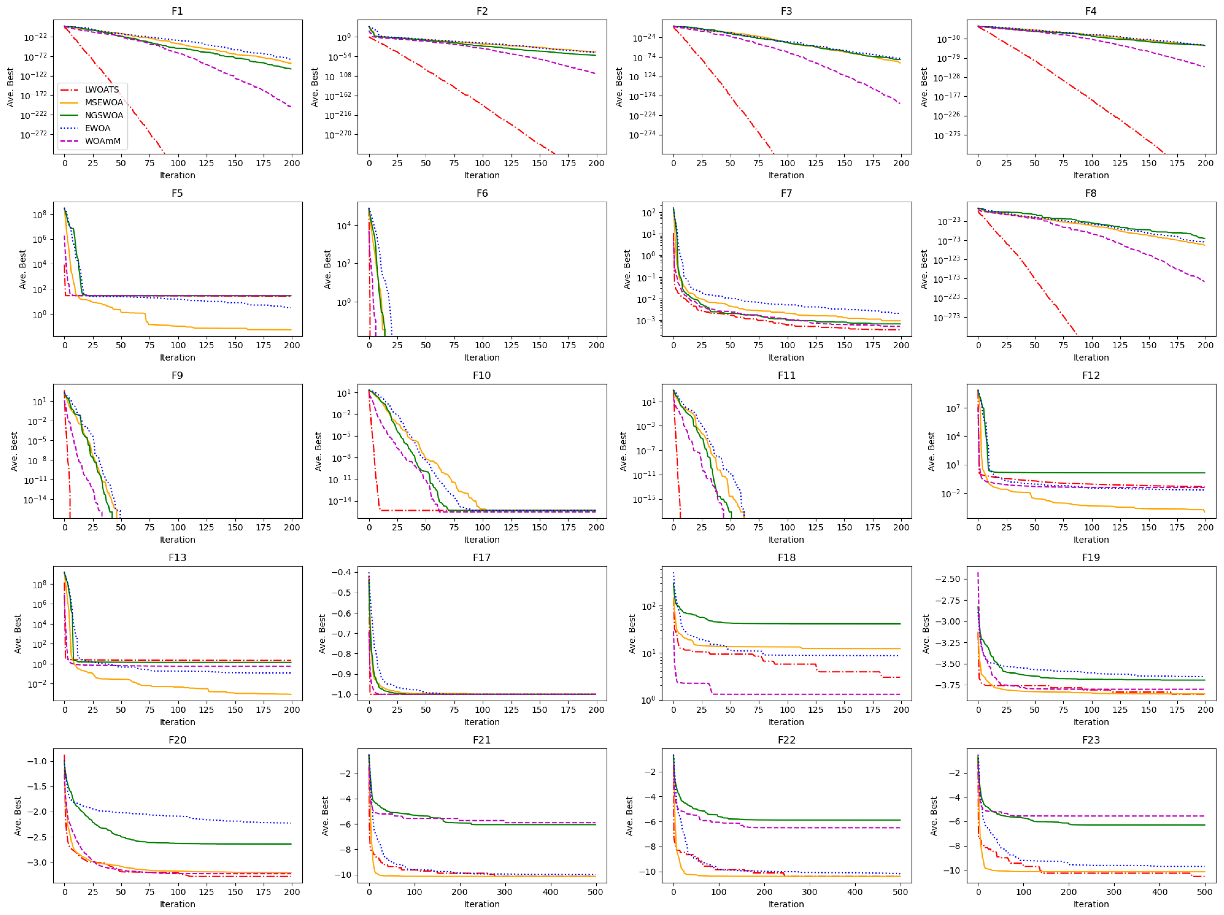
The same benchmark functions were tested for some other improved versions of WOA, including nonlinear adaptive weight and golden sine operator WOA (NGSWOA) [67], enhanced WOA (EWOA) [68], multi-strategy enhanced WOA (MSEWOA) [69], and modified mutualism phase WOA (WOAmM) [70], to validate further the performance of LWOATS. Each test was conducted for the same iterations and population size as before. The results for the first seven unimodal functions are provided in

Table A19. Performance comparison of LWOATS with improved WOA variants on unimodal functions.

Function	Result	Algorithms
		MSEWOA	NGSWOA	EWOA	WOAmM	LWOATS
F1	Best	$7.479\times {10}^{-118}$	$2.063\times {10}^{-147}$	$1.326\times {10}^{-124}$	$4.819\times {10}^{-233}$	0
	Worst	$2.301\times {10}^{-89}$	$4.824\times {10}^{-104}$	$2.654\times {10}^{-79}$	$9.769\times {10}^{-201}$	0
	Mean	$7.671\times {10}^{-91}$	$1.849\times {10}^{-105}$	$8.849\times {10}^{-81}$	$3.256\times {10}^{-202}$	0
	Std	$4.130\times {10}^{-90}$	$8.704\times {10}^{-105}$	$4.765\times {10}^{-80}$	0	0
F2	Best	$7.619\times {10}^{-67}$	$3.826\times {10}^{-70}$	$2.596\times {10}^{-59}$	0	0
	Worst	$7.397\times {10}^{-41}$	$2.286\times {10}^{-50}$	$2.528\times {10}^{-42}$	$9.846\times {10}^{-101}$	0
	Mean	$2.466\times {10}^{-42}$	$1.247\times {10}^{-51}$	$8.566\times {10}^{-44}$	$3.292\times {10}^{-102}$	0
	Std	$1.328\times {10}^{-41}$	$4.719\times {10}^{-51}$	$4.536\times {10}^{-43}$	$1.767\times {10}^{-101}$	0
F3	Best	$8.495\times {10}^{-115}$	$2.888\times {10}^{-128}$	$9.780\times {10}^{-121}$	0	0
	Worst	$1.653\times {10}^{-88}$	$1.369\times {10}^{-79}$	$1.115\times {10}^{-76}$	$3.170\times {10}^{-193}$	0
	Mean	$1.034\times {10}^{-89}$	$4.565\times {10}^{-81}$	$3.718\times {10}^{-78}$	$1.067\times {10}^{-194}$	0
	Std	$3.869\times {10}^{-89}$	$2.458\times {10}^{-80}$	$2.002\times {10}^{-77}$	0	0
F4	Best	$4.008\times {10}^{-62}$	$6.062\times {10}^{-72}$	$5.626\times {10}^{-63}$	$8.061\times {10}^{-117}$	0
	Worst	$1.575\times {10}^{-46}$	$1.810\times {10}^{-46}$	$2.139\times {10}^{-46}$	$2.954\times {10}^{-101}$	0
	Mean	$6.313\times {10}^{-48}$	$6.665\times {10}^{-48}$	$1.267\times {10}^{-47}$	$1.345\times {10}^{-102}$	0
	Std	$2.864\times {10}^{-47}$	$3.255\times {10}^{-47}$	$4.096\times {10}^{-47}$	$5.459\times {10}^{-102}$	0
F5	Best	$2.641\times {10}^{-10}$	$2.841\times {10}^1$	$1.778\times {10}^{-3}$	$2.798\times {10}^1$	$2.606\times {10}^1$
	Worst	$8.751\times {10}^{-1}$	$2.885\times {10}^1$	$2.877\times {10}^1$	$2.880\times {10}^1$	$2.886\times {10}^1$
	Mean	$5.369\times {10}^{-2}$	$2.874\times {10}^1$	$3.106\times {10}^0$	$2.853\times {10}^1$	$2.746\times {10}^1$
	Std	$1.605\times {10}^{-1}$	$1.011\times {10}^{-1}$	$8.550\times {10}^0$	$2.112\times {10}^{-1}$	$9.583\times {10}^{-1}$
F6	Best	0	0	0	0	0
	Worst	0	0	0	0	0
	Mean	0	0	0	0	0
	Std	0	0	0	0	0
F7	Best	$3.500\times {10}^{-5}$	$7.000\times {10}^{-6}$	$1.510\times {10}^{-4}$	$3.400\times {10}^{-5}$	$8.433\times {10}^{-6}$
	Worst	$4.348\times {10}^{-3}$	$2.942\times {10}^{-3}$	$1.208\times {10}^{-2}$	$2.125\times {10}^{-3}$	$1.270\times {10}^{-3}$
	Mean	$9.490\times {10}^{-4}$	$6.780\times {10}^{-4}$	$2.109\times {10}^{-3}$	$5.250\times {10}^{-4}$	$3.269\times {10}^{-4}$
	Std	$1.012\times {10}^{-3}$	$7.170\times {10}^{-4}$	$2.380\times {10}^{-3}$	$4.640\times {10}^{-4}$	$2.579\times {10}^{-4}$

. LWOATS performs better than the other algorithms in most cases, except F5. However, in the case of F5, only NGSWOA and EWOA manage to escape local minima, since the other algorithms seem to get trapped (see Figure A3).

On the high-dimension multimodal functions, LWOATS demonstrates a superior performance on F8, coupled with faster convergence rates on F9 and F11. However, on F10, LWOATS is outperformed by WOAmM, which occasionally identifies the global minimum during some tests. Nonetheless, LWOATS matches the performance of other algorithms in terms of achieving similar results but with faster convergence, as illustrated in the diagrams shown in Figure A3. LWOATS behaves poorly on F12 and F13, and thus is outperformed by most of the other versions.

In the case of the fixed-dimension multimodal functions, LWOATS demonstrates a superior performance, providing better results with lower standard deviations in most scenarios. In the case of Shekel’s functions, MSEWOA is the only algorithm that approaches the performance of LWOATS, yielding results close to the global minimum, yet still not surpassing LWOATS. The only exception where LWOATS does not lead is in the scenario involving F14, where its performance is comparatively weaker.

The Wilcoxon’s test results for unimodal and high-dimensional multimodal functions, as well as for the fixed-dimension multimodal functions, are summarized in

Table A21. Results of Wilcoxon statistical test for unimodal and high-dimensional multimodal functions for LWOATS and improved WOA variants.

Comparison	${\mathit{R}}^{+}$	${\mathit{R}}^{-}$	+	−	=	Decision
LWOATS vs. WOAmM	2683	1765	5	5	3	++++===+=−=−−
LWOATS vs. EWOA	2771	1414	6	4	3	++++−=++===−−
LWOATS vs. MSEWOA	2709	1476	6	4	3	++++−=++===−−
LWOATS vs. NGSWOA	3379	806	7	5	1	+++++==+===+−

and

Table A24. Results of Wilcoxon statistical test for fixed-dimension multimodal functions for LWOATS and improved WOA variants.

Comparison	${\mathit{R}}^{+}$	${\mathit{R}}^{-}$	+	−	=	Decision
LWOATS vs. WOAmM	2771	1414	6	3	1	−−+=−+++++
LWOATS vs. EWOA	3307	878	7	1	2	−++=+++=++
LWOATS vs. MSEWOA	3060	1125	6	1	3	−++=+++==+
LWOATS vs. NGSWOA	4101	84	9	0	1	+++=++++++

, respectively. Overall, LWOATS outperforms or shows a competitive performance over WOAmM in 15 functions out of 23, shows a competitive performance in 4, and underperforms in 8. Compared to EWOA, LWOATS performs better or shows a competitive performance in 18 functions and worse in 5. It also behaves similarly to the previous comparison when compared to MSEWOA and NGSWOA. The p-values for these tests are summarized in Table A21 and

Table A25. Wilcoxon’s p-values for each comparison of LWOATS and improved WOA variants for the fixed-dimension multimodal functions.

Function	LWOATS vs. WOAmM	LWOATS vs. EWOA	LWOATS vs. MSEWOA	LWOATS vs. NGSWOA
F14	$9.313\times {10}^{-9}$	$3.725\times {10}^{-9}$	$1.863\times {10}^{-9}$	$9.903\times {10}^{-5}$
F15	$3.790\times {10}^{-6}$	$1.863\times {10}^{-9}$	$6.147\times {10}^{-8}$	$9.313\times {10}^{-9}$
F16	$5.588\times {10}^{-9}$	$1.863\times {10}^{-9}$	$1.863\times {10}^{-9}$	$1.863\times {10}^{-9}$
F17	$1.000\times {10}^0$	$1.000\times {10}^0$	$1.000\times {10}^0$	$1.000\times {10}^0$
F18	$6.665\times {10}^{-4}$	$1.863\times {10}^{-9}$	$1.863\times {10}^{-9}$	$1.863\times {10}^{-9}$
F19	$3.790\times {10}^{-6}$	$1.992\times {10}^{-6}$	$3.790\times {10}^{-6}$	$1.863\times {10}^{-9}$
F20	$5.055\times {10}^{-4}$	$3.725\times {10}^{-9}$	$3.454\times {10}^{-2}$	$1.863\times {10}^{-9}$
F21	$1.863\times {10}^{-9}$	$1.293\times {10}^{-1}$	$6.850\times {10}^{-1}$	$1.863\times {10}^{-9}$
F22	$4.712\times {10}^{-7}$	$4.971\times {10}^{-2}$	$1.706\times {10}^{-1}$	$3.856\times {10}^{-7}$
F23	$1.863\times {10}^{-8}$	$2.987\times {10}^{-3}$	$1.366\times {10}^{-2}$	$6.147\times {10}^{-8}$

. These results highlight the efficiency and superiority of our algorithm, even when compared to state-of-the-art improved variants of the WOA algorithm.

3.4. Performance on F5, F12, and F13

It is worth investigating, however, the poor performance on some test cases such as F5, F12, and F13. Rosenbrock (F5) forms a long, curved “banana” valley whose gradient is almost orthogonal to the valley’s axis. Levy jumps with a fixed step size often overshoot the ridge, while Nelder–Mead assumes locally star-shaped basins and therefore drifts across, rather than along, the curved floor. The penalized benchmarks F12 and F13 add a second difficulty: a broad, flat plateau created by the penalty term $U(x_i,·)$ and a tiny feasible basin around $\mathbf{x}=1$. Many whales quickly settle on different plateaus that look equally promising. The tabu list then stores near-duplicate locations, elite diversity collapses, and the population lacks the momentum to jump the steep penalty walls.

Two complementary modifications appear promising and will be explored in future work:

1. Curvature-aware local search: Replacing Nelder–Mead with a quasi-Newton or BFGS step once the elite set has converged could guide the search along the Rosenbrock valley rather than across it.

2. Dynamic exploration pressure: Adapting the Levy flight scale and/or tabu list length based on population fitness variance would allow larger corrective jumps when the swarm stagnates on penalized plateaus, yet still shrink steps for fine-tuning near the optimum.

These planned enhancements are expected to improve robustness on Rosenbrock-type valleys and heavily penalized landscapes without affecting LWOATS’s strong performance on the remaining benchmarks.

3.5. Influence of Tabu Search and Elite Solutions in Exploitation

The use of memory elements and logic such as Tabu Search, in the proposed LWOATS algorithm, leads to significant benefits for the optimization approach, especially in complex problems. These mechanisms prevent the optimization process from revisiting previously explored poor solutions, thereby promoting exploration. This prevents the algorithm from oscillating between local optima, thus forcing it to explore new areas of the search space that are not marked as “tabu”, ultimately avoiding premature convergence to suboptimal solutions.

In addition to Tabu Search, by keeping a list of good solutions (elites), LWOATS ensures that the best solutions are maintained during the exploration process and are not lost. The reintroduction of these solutions directs the population of the LWOATS toward high-quality solutions without re-exploring low-quality regions. Therefore, LWOATS focuses the search on the most promising areas of the search space, balancing exploration and exploitation. Even if some members of the population are misled into suboptimal regions, elites are protected and can serve as a guide to bring the population back on track, preventing the solution quality from degrading.

Shekel’s functions (F21, F22, and F23) are challenging benchmarking problems due to their multimodality and narrow basins of attraction. These functions have many local minima, and many traditional and fundamental algorithms struggle to find the global best, even after many evaluations, especially as the dimensionality increases from F21 to F23. In order to evaluate the performance of LWOATS, we executed two different implementations: one with the integration of tabu and elite memory mechanisms, and the other without. The results are presented in Figure 6.

As illustrated in the figure, the implementation without the memory mechanisms requires more evaluations to improve the solution’s quality gradually. In the cases of F21, F22, and F23, although the algorithm eventually converges, it does so much more slowly and often to a solution that is far from the global optimum. On the contrary, the implementation with the memory mechanisms rapidly converges to a near-optimal solution, often within a few thousand evaluations. This demonstrates the efficacy of the memory elements in guiding the search to optimal or near-optimal solutions efficiently.

3.6. Runtime Complexity

LWOATS is a complex algorithm, and thus the runtime complexity estimation depends on several critical processes such as initialization, fitness evaluation, population update, and local search optimization. The first phase of the algorithm begins by initializing a population of p agents, resulting in a computational complexity of $O(p\times d)$ due to the random generation of positions across d dimensions. The fitness evaluation of each individual involves computing a given function, totaling $O(p\times d)$, per iteration.

The sorting population and selecting elite solutions procedures can be approximately estimated by a complexity equivalent to $O(p\times logp)$. The selection contribution is negligible since it is $O\left(E\right)$, where E are the elite solutions, which is equal to ${\displaystyle \frac{p}{10}}$ in our case. So the term that is the most significant is from the sorting and is equal to $O(p\times logp)$.

The whale optimization updates (individual and social learning mechanisms) contribute with a total complexity of $O(p\times d)$ per iteration. Furthermore, elite solutions undergo local search utilizing the Nelder–Mead algorithm, with complexity $O({\displaystyle \frac{p}{10}}\times N\times d)$, and N are the Nelder–Mead iterations. Lastly, the Tabu Search operations contribute with a total complexity of $O(E\times T_{size})=$$O({\displaystyle \frac{p}{10}}\times {\displaystyle \frac{p}{2}})$, where $T_{size}$ is the tabu list size which is equal to ${\displaystyle \frac{p}{2}}$.

Consequently, summing these complexities across i iterations gives a total runtime complexity for the LWOATS of

$$O(i\times (d\times p+d\times plogp+p^2)),$$

(11)

since the other parameters do not contribute significantly. This final formula (11) encapsulates the multiple layers of computational effort required for the algorithm to converge to an optimal solution.

4. LWOATS for Engineering Problems

We tested LWOATS’s performance on seven different real-world optimization problems using the death penalty as the simplest constraint method through which a big objective value is applied in the case of minimization [71]: the spring tension/compression design, the pressure vessel design, the welded beam design, the weight minimization of a speed reducer, the gear train design, the three-bar truss design, and the economic load dispatch for 3 and 13 units. In each of the following subsections, the mathematical formulation of these problems is presented as obtained from the literature [64,70,72]. The parameter settings for LWOATS are the same as those in Table 1. The results obtained from LWOATS are compared with others from the literature.

4.1. Tension/Compression Spring Design

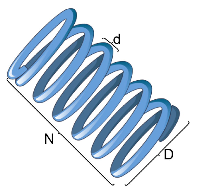
The main objective of the tension/compression spring design optimization problem is to minimize the weight of a mechanical spring by finding the best solution to three variables (Figure 7): wire diameter d, mean coil diameter D, and number of active coils N. The results from LWOATS are presented in

Table 5. Spring design problem. LWOATS values are shown in bold.

Algorithm	d	D	N	Best $\mathcal{W}$
LWOATS	0.05168889	0.35671364	11.28920611	0.012665233
HHO [73]	0.051796393	0.359305355	11.138859	0.012665443
GWO [11]	0.05169	0.356737	11.28885	0.012666
MFO [76]	0.051994457	0.36410932	10.868421862	0.0126669
GJO [64]	0.0515793	0.354055	11.4484	0.01266752
BAT [75]	0.05169	0.35673	11.2885	0.01267
WSOA [77]	0.0512	0.3441	12.0663	0.01267
CPSO [74]	0.051728	0.357644	11.244543	0.0126747
WOA [22]	0.051207	0.345215	12.004032	0.0126763
MVO [78]	0.05	0.315956	14.22623	0.0144644

and compared with the results obtained from other metaheuristic approaches such as WOA [22], GWO [11], the golden jackal optimization algorithm (GJO) [64], the Harris hawks optimization algorithm (HHO) [73], the co-evolutionary particle swarm optimization algorithm (CPSO) [74], BAT [75], the moth–flame optimization algorithm (MFO) [76], the hybrid whale–seagull optimization algorithm (WSOA) [77], and the multi-verse optimization algorithm (MVO) [78].

The mathematical formulation of this problem is presented by the set of equations and constraints in Appendix E.1. The algorithm was evaluated for 10 agents and 100 iterations, while the max iterations for Nelder–Mead were set to 100. LWOATS outperforms all of the other metaheuristic algorithms and achieves better results regarding the minimization of the weight cost function for the spring. The results in Table 5 are sorted from best to worst. Because Table 5 includes only the raw costs, we also report the percentage deviation from LWOATS’s best value, defined as

$$\Delta \%={\displaystyle \frac{C_{\mathrm{alg}}-C_{\mathrm{best}}}{C_{\mathrm{best}}}}\times 100\%,$$

(12)

where with C we denote the final cost.

On the spring design test (

Table 6. Percentage weight increase over LWOATS for the spring design problem.

Algorithm	HHO	GWO	MFO	GJO	BAT	WSOA	CPSO	WOA	MVO
$\Delta \%$	0.0017	0.0061	0.0132	0.0181	0.0376	0.0376	0.0747	0.0874	14.206

), HHO is practically on par with LWOATS, yielding a spring only 0.002% heavier than the optimum. Three further algorithms (GWO, MFO, and GJO) form a “close” tier, each deviating by <0.02%. A second cluster (BAT and WSOA, 0.04%; CPSO, 0.07%; and baseline WOA, 0.09%) incurs sub-0.1% penalties. By contrast, the classical MVO trails badly, adding >14% to the weight. LWOATS sets the benchmark, a few modern metaheuristics nearly match it, a mid-tier pays modest costs, and legacy methods fall far behind, underscoring the proposed hybrid’s consistent edge across disparate spring designs.

4.2. Welded Beam Design

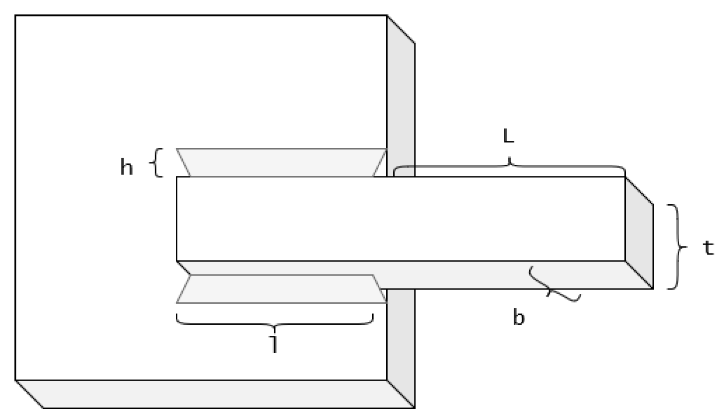
The welded beam design is a very well-known optimization problem in which the main goal is to find the best values for the thickness of weld (h), bar length (l), height (t), and thickness (b), as shown in Figure 8. These parameters are subject to the shear stress ($\tau$), bending stress ($\theta$), beams’ end deflection ($\delta$), and other constraints, as formulated by Equation (A9). Many researchers have solved this problem with their proposed metaheuristic approach. Yildiz employed an improved version of WOA, namely HWOANM [79], while Mirjalili S. proposed many algorithms through which he solved many engineering problems, including the welded beam design, such as MVO [78], GWO [11], and WOA [22]. Chopra and Ansari utilized GJO, while He Wang proposed an improved version of PSO [74] (CPSO). Other approaches include WSOA [77], the gravitational search algorithm (GSA) [80], GA [81], and the society and civilization optimization algorithm (SCA) [82]. LWOATS is evaluated for a size of 30 agents and 500 iterations for 20 independent runs. The best result obtained by LWOATS outperforms all the other approaches (

Table 7. Welded beam design problem.

Algorithm	h	l	t	b	Best Cost
LWOATS	0.20572986	3.47048573	9.03661999	0.20573003	1.724854
HWOANM [79]	0.2057	3.4714	9.0366	0.2057	1.72491
MVO [78]	0.205463	3.473193	9.044502	0.205695	1.72645
GWO [11]	0.205676	3.478377	9.03681	0.205778	1.72624
GJO [64]	0.20562	3.4719	9.0392	0.20572	1.72522
WOA [22]	0.205396	3.484293	9.037426	0.206276	1.730499
CPSO [74]	0.202369	3.544214	9.048210	0.205723	1.73148
WSOA [77]	0.1919	3.7633	9.1090	0.2054	1.7519
GSA [80]	0.182129	3.856979	10.00000	0.202376	1.879952
GA [81]	0.2489	6.1730	8.1789	0.2533	2.43312
SCA [82]	0.2440	6.238	8.2886	0.2446	2.3854

).

The normalized values are given in

Table 8. Percentage cost increase over LWOATS for the welded beam design.

Algorithm	HWOANM	GJO	GWO	MVO	WOA	CPSO	WSOA	GSA	SCA	GA
$\Delta \%$	0.003	0.021	0.08	0.09	0.33	0.38	1.57	9.0	38.3	41.1

. HWOANM is effectively tied with LWOATS, exceeding the optimum by 0.003%. A first tight cluster (GJO, GWO, and MVO) remains within 0.1% of the best cost (0.02%, 0.08%, and 0.09%, respectively). The two further recent methods, WOA and CPSO, are still very competitive, incurring only 0.33% and 0.38% penalties. The performance then drops to a mid-tier: WSOA is 1.57% costlier, while the classical GSA lags at 9%. Legacy evolutionary approaches (SCA and GA) trail far behind, adding roughly 38–41% to fabrication costs. LWOATS and one modern hybrid sit at the top, several contemporary metaheuristics follow with marginal losses, and older algorithms suffer substantively larger penalties.

4.3. Pressure Vessel Design

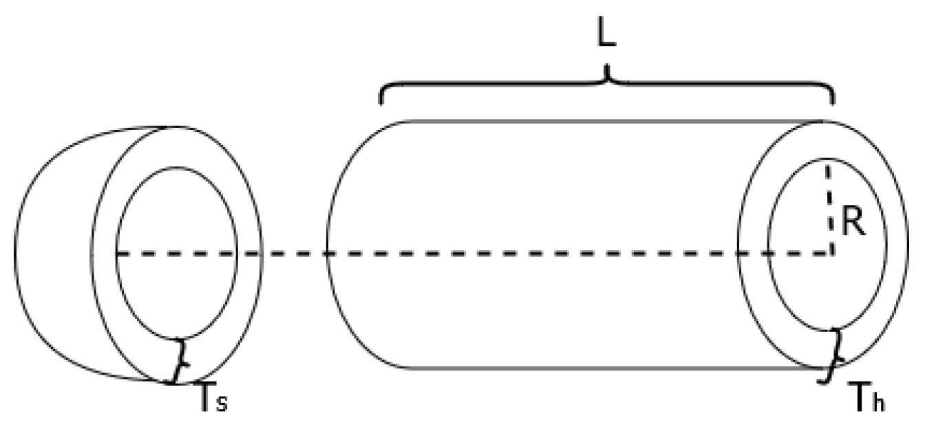
Another engineering design problem that traditional approaches often fail to solve efficiently is minimizing the fabrication cost of a pressure vessel, as shown in Figure 9. The parameters that need to be optimized are the shell thickness (Ts), the inner radius (R), the head thickness (Th), and the length of the cylindrical section (L). The constraints under which this problem is mathematically formulated are presented by Equation (A8). Again, LWOATS is evaluated for 10 agents, 100 iterations, and 20 independent runs. The best result obtained by LWOATS outperforms all the other proposed solutions compared with it, including HHO [73], WSOA [77], GJO [64], GWO [11], MFO [76], MVO [78], GSA [80], CPSO [74], and WOA [22], as presented in

Table 9. Pressure vessel design problem.

Algorithm	${\mathit{T}}_{\mathit{s}}$	${\mathit{T}}_{\mathit{h}}$	R	L	Best Cost
LWOATS	0.77816867	0.38464916	40.31961884	200	5885.3329
GJO [64]	0.7782955	0.3848046	40.32187	200	5887.071123
WSOA [77]	0.8056	0.4081	41.7401	181.1285	5964.6114
HHO [73]	0.81758383	0.4072927	42.09174576	176.7196352	6000.46259
GWO [11]	0.812500	0.434500	42.089181	176.758731	6051.5639
MFO [76]	0.8125	0.4375	42.098445	176.636596	6059.7143
WOA [22]	0.812500	0.437500	42.0982699	176.638998	6059.7410
MVO [78]	0.8125	0.4375	42.0907382	176.738690	6060.8066
CPSO [74]	0.8125	0.4375	42.091266	176.746500	6061.0777
GSA [80]	1.1250	0.6250	55.9886598	84.4542025	8538.8359

.

Table 10. Percentage cost increase over LWOATS for the pressure vessel problem.

Algorithm	GJO	WSOA	HHO	GWO	MFO	WOA	MVO	CPSO	GSA
$\Delta \%$	0.03	1.35	1.96	2.83	2.96	2.96	2.98	2.99	45.09

provides the normalized results. GJO trails LWOATS by only 0.03%, whereas the next cluster (WSOA, HHO, and GWO) lands within the 2–3% band: WSOA is 1.35% more expensive, HHO 1.96%, and GWO 2.83%. MFO, WOA, and MVO all sit at roughly the same level, ≈3% above the optimum, while CPSO is only a hair worse at 2.99%. Beyond that, the classical GSA lags badly, adding a prohibitive 45% to the fabrication cost. This gradient illustrates both the competitiveness of LWOATS against state-of-the-art hybrids and its pronounced advantage over earlier optimization paradigms.

4.4. Three-Bar Truss Design

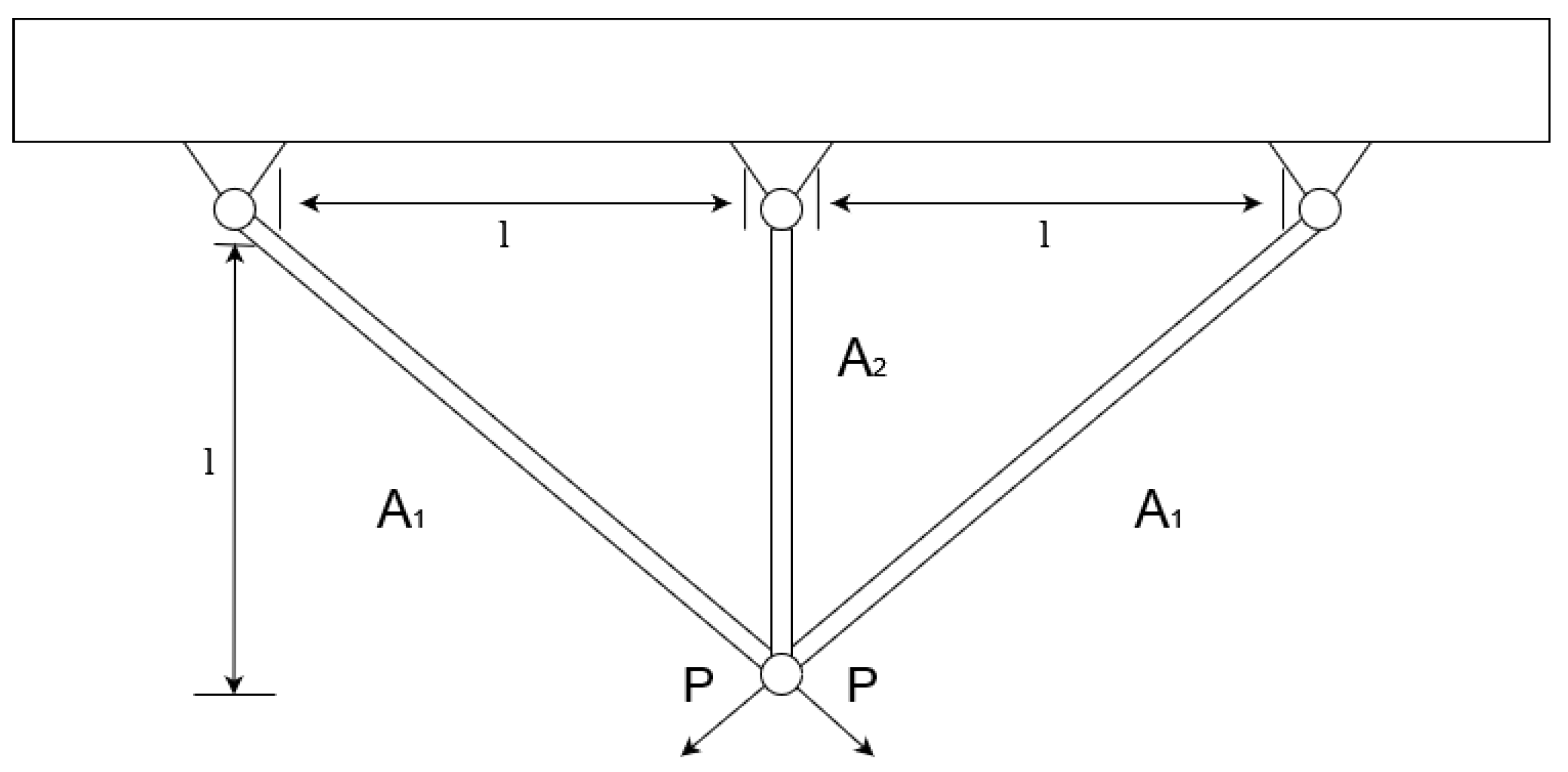
A highly constrained problem is minimizing the burden of a three-bar structure, as illustrated in Figure 10. Such truss optimization problems are usually subject to many constraints. Stress, buckling, and deflection are the ones for each bar in the case of this design problem. LWOATS were executed for 10 agents, 100 iterations, and 20 independent runs.

Table 11. Three-bar truss design problem.

Algorithm	${\mathit{A}}_1$	${\mathit{A}}_2$	Best Cost
LWOATS	0.78867344	0.40825308	263.89584339
HHO [73]	0.788662816	0.40828313383	263.89584348
ALO [83]	0.788662816000317	0.408283133832901	263.895843488
GJO [64]	0.788657163482708	0.408299125193296	263.8958439
MVO [78]	0.78860276	0.408453070	263.8958499
MBA [84]	0.7885650	0.4085597	263.8958522
GOA [85]	0.788897555578973	0.407619570115153	263.895881496069
MFO [76]	0.788244771	0.409466905784741	263.8959797
SCA [82]	0.78669	0.41426	263.9348
CS [86]	0.78867	0.40902	263.9716

compares the results with other algorithms. On this problem, six modern methods (HHO, ALO, GJO, MVO, MBA, GOA, and MFO) are essentially indistinguishable from LWOATS, their costs differing by less than one-ten-thousandth of a percent. Only the older evolutionary schemes show a visible gap: SCA is 0.015% heavier and CS 0.029%. Thus, while LWOATS retains the top spot, nearly all recent hybrids achieve near-identical optima on this low-dimensional, tightly constrained structure, whereas legacy algorithms begin to drift away.

4.5. Gear Train Design

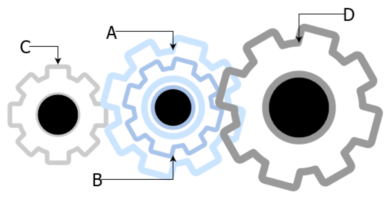
The gear train design problem is a discrete optimization problem in which the main goal is to determine the optimum number of teeth for each one of the gears presented in Figure 11. LWOATS provides competitive results against ALO [83] and CS [86] while outperforming the rest of the algorithms as illustrated in

Table 12. Gear train design problem.

Algorithm	${\mathit{n}}_{\mathit{a}}$	${\mathit{n}}_{\mathit{b}}$	${\mathit{n}}_{\mathit{c}}$	${\mathit{n}}_{\mathit{d}}$	Best Cost
LWOATS	43	19	16	49	$2.7009\times {10}^{-12}$
ALO [83]	49	19	16	43	$2.7009\times {10}^{-12}$
CS [86]	43	16	19	49	$2.7009\times {10}^{-12}$
ABC [87]	19	16	44	49	$2.78\times {10}^{-11}$
GA [88]	33	14	17	50	$1.362\times {10}^{-9}$
ALM [89]	33	15	13	41	$2.1469\times {10}^{-8}$

. The best of the remainder, ABC, is already $9.29\times {10}^2$% above the optimum, while GA and ALM lag by $5.03\times {10}^4$ and $7.95\times {10}^5$, respectively. This showcases the fact that LWOATS can also handle discrete optimization problems efficiently.

4.6. Speed Reducer

A challenging optimization problem is the minimization of a reducer [90] under various constraints (surface pressure, lateral deflection of the shaft, bending stress of the gear, and pressure in the shaft) as they are mathematically formulated by Equation (A11). In this design problem, seven different variables need to be determined to find the optimum cost: the face width $x_1$, the tooth module $x_2$, the pinion’s teeth number $x_3$ (integer), the length of the first shaft (between bearings) $x_4$, the length of the second shaft $x_5$, and the diameters of the first and second shaft, $x_6$, $x_7$, respectively. LWOATS is compared with various algorithms, chief among them the improved seagull optimization algorithm (ISOA) [90], CS [86], GJO [64], the spotted hyena optimizer (SHO) [91], the modified flower pollination algorithm (MFPA) [92], and the evolutionary algorithm (EA) [93]. LWOATS achieves competitive results, outperforming most of the other proposed algorithms except ISOA, which achieves a better cost, as illustrated in

Table 13. Speed reducer problem.

Algorithm	${\mathit{x}}_1$	${\mathit{x}}_2$	${\mathit{x}}_3$	${\mathit{x}}_4$	${\mathit{x}}_5$	${\mathit{x}}_6$	${\mathit{x}}_7$	Best Cost
ISOA [90]	3.40385	0.7	17	7.74585	7.76495	3.32186	5.25780	2973.9175
LWOATS	3.50007075	0.7	17	7.30298402	7.71628516	3.35025427	5.28666227	2994.5614
GJO [64]	3.500003	0.7	17	7.321686	7.72122	3.35025	5.28665	2994.80495
CS [86]	3.5015	0.7	17	7.6050	7.8181	3.3520	5.2875	3000.981
MFPA [92]	3.5	0.7	17	7.3	7.8005	3.35021	5.28668	2996.219
SHO [91]	N/A	N/A	N/A	N/A	N/A	N/A	N/A	2998.550
EA [93]	3.506163	0.700831	17	7.46018	7.962143	3.3629	5.3090	3025.005

. More specifically, ISOA currently holds the best-known cost. LWOATS falls short by only 0.69%, effectively matching the performance of GJO (0.70%) and MFPA (0.75%). SHO and CS remain in the sub-1% band (0.83% and 0.91%, respectively), while the evolutionary baseline EA trails at 1.72%. SHO is marginally worse at 0.83%, and the evolutionary baseline EA lags by 1.7%.

4.7. Economic Load Dispatch

Economic load dispatch (ELD) is an optimization problem that is very essential in power system planning; ELD is used to allocate, in the best possible way, the required power between the available generating units that would satisfy load demand effectively and the various operational constraints of the power units. ELD is such a complex problem that traditional approaches often fail to find the optimum solution. Thus, metaheuristic methods like swarm intelligence are often utilized to achieve the best results. The total fuel cost that we try to minimize can be mathematically modeled by the following equation:

$$C_i\left(P_i\right)=a_i+b_i{P}_i+c_i{P}_i^2+\left|d_i\times sin\left[e_i\times \left(P_i^{min}-P_i\right)\right]\right|,$$

(13)

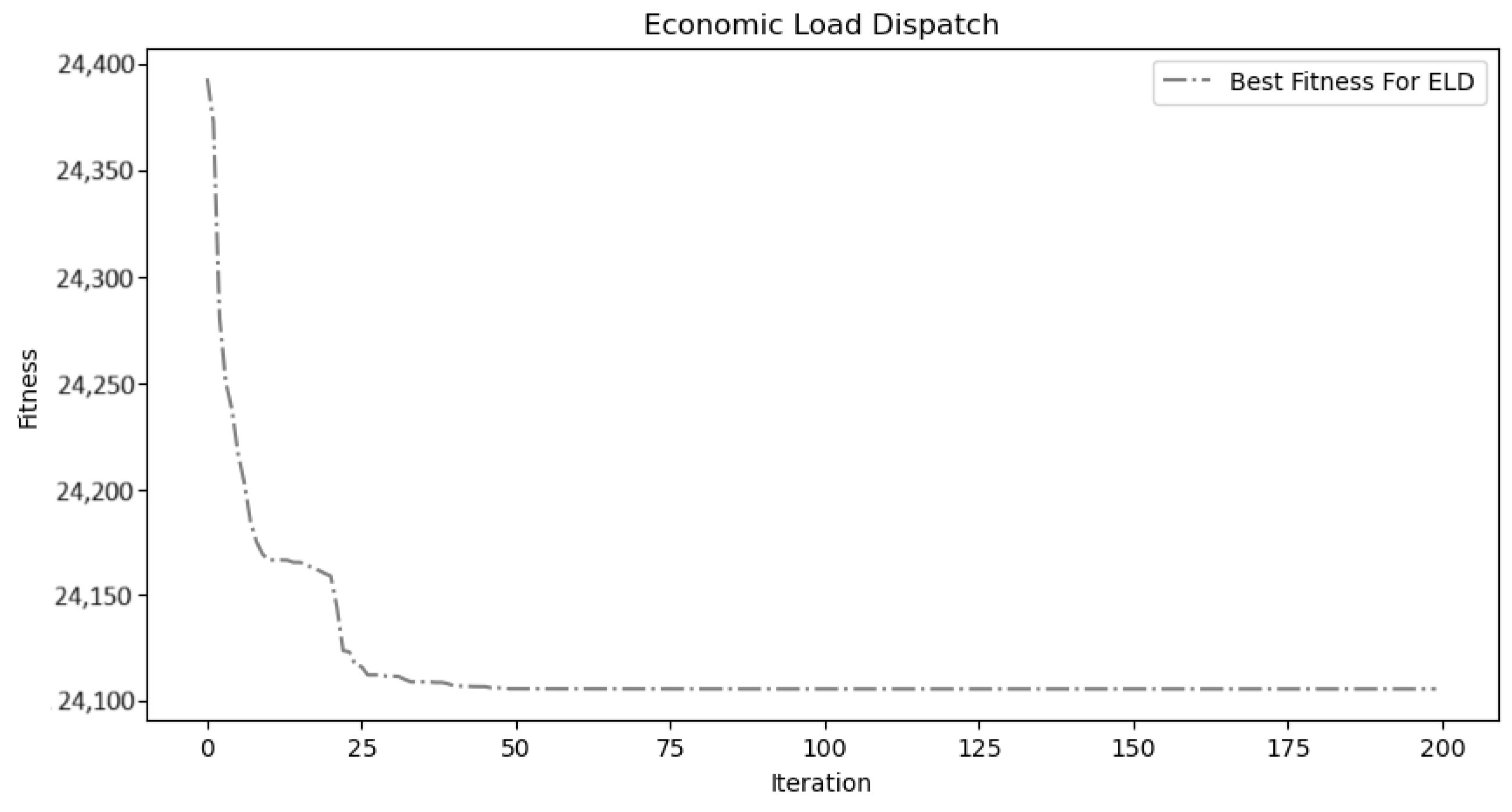
where the indices are summed. $a_i$, $b_i$, and $c_i$ are the function coefficients, while $d_i$ and $e_i$ are the coefficients of the valve-point loading effects. The values of these parameters are given in

Table 14. Unit data for the 13-unit ELD test system with the valve-point loading effects.

Unit No.	${\mathit{P}}_{\mathbf{min}}$ (MW)	${\mathit{P}}_{\mathbf{max}}$ (MW)	a	b	c	d	e
1	0	680	550	8.1000	0.00028	300	0.0350
2	0	360	309	8.1000	0.00056	200	0.0420
3	0	360	307	8.1000	0.00056	200	0.0420
4	60	180	240	7.7400	0.00324	150	0.0630
5	60	180	240	7.7400	0.00324	150	0.0630
6	60	180	240	7.7400	0.00324	150	0.0630
7	60	180	240	7.7400	0.00324	150	0.0630
8	60	180	240	7.7400	0.00324	150	0.0630
9	60	180	240	7.7400	0.00324	150	0.0630
10	40	120	126	8.6000	0.00284	100	0.0840
11	40	120	126	8.6000	0.00284	100	0.0840
12	55	120	126	8.6000	0.00284	100	0.0840
13	55	120	126	8.6000	0.00284	100	0.0840

. Following this approach, we utilized LWOATS to determine the best values for the $P_i$’s in Equation (13) and thus the minimum fuel cost required with a load demand of 2520 MW for the 13-unit ELD system. The results obtained by LWOATS are summarized in

Table 15. Results obtained by LWOATS for the 13-unit ELD problem.

Unit No.	LWOATS	Unit No.	LWOATS
1	680	8	159.65872993
2	360	9	109.82395927
3	352.78337842	10	114.55725804
4	159.66741217	11	42.55544494
5	109.82971340	12	55.51997359
6	159.73314659	13	56.11272851
7	159.75833436
Best fuel cost: 24,105.684 USD/h

, while the convergence curve is illustrated in Figure 12.

The best and mean fuel cost obtained by LWOATS are compared with other algorithms such as ACO [94], $\beta$-GWO [95], the salp swarm algorithm and a hybrid version of it (SSA/HSSA) [96], and the tournament-based harmony search algorithm (THS) [97]. The results presented in

Table 16. Comparison of the results for a 13-unit system with 2520 MW power demand.

Algorithm	Best Cost (USD/h)	Mean Cost (USD/h)
LWOATS	24,105.68	24,222.98
THS [97]	24,164.06	24,195.21
$\beta$-GWO [95]	24,164.10	24,164.20
HSSA [96]	24,164.21	24,164.47
SSA [96]	24,168.97	24,295.45
ACO [94]	24,174.39	24,211.09

, indicate that LWOATS outperforms the rest of the algorithms regarding the minimum fuel cost that can be achieved. LWOATS offers a 0.24% gain relative to the next best algorithm’s results. However, the mean value is worse than most of the values obtained from the other solutions. LWOATS was evaluated for 100 agents and 200 iterations for 20 independent runs. The maximum iterations for the Nelder–Mead simplex algorithm were set to 100. The approximate time to execute each iteration was 22 s.

5. Conclusions

In this work, we propose a new enhanced version of the Whale Optimization Algorithm (WOA). The hybridization of WOA with the Nelder–Mead-based local search, the memory elements of the Tabu Search algorithm, and the integration of Levy flights addresses the slow convergence and suboptimal exploration and exploitation characteristics of the original WOA. The proposed LWOATS is rigorously evaluated using 23 benchmark functions, demonstrating significant improvements in both exploration and exploitation capabilities. To further validate these results, Wilcoxon rank-sum statistical tests were performed. Additionally, the memory elements’ contribution was extensively analyzed by visualizing their impact on the convergence of LWOATS in challenging functions like Shekel’s functions. The results from all the above tests indicate that LWOATS achieves substantially faster convergence compared to other well-established algorithms in the literature, such as PSO, GWO, DE, and the original WOA. LWOATS also presents a better or competitive performance against advanced algorithms such as SaDE, JADE, iL-SHADE, and jSO. Additionally, the comparison of LWOATS with state-of-the-art improved WOA variations reveals that our approach surpasses the performance of these algorithms in most cases or performs competitively.

Further evaluation of LWOATS was conducted on six well-known constraint (and non-) engineering problems, comparing its performance with the results of other algorithms in the literature. LWOATS outperforms other approaches, providing results that achieve better minimum scores each time, showing that it can handle demanding problems effectively. Furthermore, the application of LWOATS in a real-case 13-dimensional electrical engineering problem (ELD) reveals its capability of solving high-dimensional and complex search space engineering problems.

Multiple promising directions can be followed for future work. We propose the application of LWOATS in machine learning applications, such as feature extraction, weight optimization in neural networks, or more practical scenarios such as path planning for unmanned vehicles (UAVs, UGVs, etc.) and obstacle avoidance scenarios.

References

1. Razmjooy, N.; Ashourian, M.; Foroozandeh, Z. Metaheuristics and Optimization in Computer and Electrical Engineering; Springer: Berlin/Heidelberg, Germany, 2021; Volume 696. [Google Scholar] [CrossRef]
2. Sharma, M.; Kaur, P. A comprehensive analysis of nature-inspired meta-heuristic techniques for feature selection problem. Arch. Comput. Methods Eng. 2021, 28, 1103–1127. [Google Scholar] [CrossRef]
3. Salcedo-Sanz, S. Modern meta-heuristics based on nonlinear physics processes: A review of models and design procedures. Phys. Rep. 2016, 655, 1–70. [Google Scholar] [CrossRef]
4. Sigmund, O. On the usefulness of non-gradient approaches in topology optimization. Struct. Multidiscip. Optim. 2011, 43, 589–596. [Google Scholar] [CrossRef]
5. Dokeroglu, T.; Sevinc, E.; Kucukyilmaz, T.; Cosar, A. A survey on new generation metaheuristic algorithms. Comput. Ind. Eng. 2019, 137, 106040. [Google Scholar] [CrossRef]
6. Kennedy, J.; Eberhart, R. Particle swarm optimization. In Proceedings of the ICNN’95-International Conference on Neural Networks, Perth, Australia, 27 November–1 December 1995; Volume 4, pp. 1942–1948. [Google Scholar] [CrossRef]
7. Dorigo, M.; Birattari, M.; Stutzle, T. Ant colony optimization. IEEE Comput. Intell. Mag. 2006, 1, 28–39. [Google Scholar] [CrossRef]
8. Holland, J.H. Genetic algorithms. Sci. Am. 1992, 267, 66–73. [Google Scholar] [CrossRef]
9. Mitchell, M. An Introduction to Genetic Algorithms; MIT Press: Cambridge, MA, USA, 1998. [Google Scholar]
10. Yang, X.S. A new metaheuristic bat-inspired algorithm. In Nature Inspired Cooperative Strategies for Optimization, NICSO; Springer: Berlin/Heidelberg, Germany, 2010; pp. 65–74. [Google Scholar] [CrossRef]
11. Mirjalili, S.; Mirjalili, S.M.; Lewis, A. Grey wolf optimizer. Adv. Eng. Softw. 2014, 69, 46–61. [Google Scholar] [CrossRef]
12. Yang, X.S. Flower pollination algorithm for global optimization. In Proceedings of the International Conference on Unconventional Computing and Natural Computation, Orléans, France, 3–7 September 2012; pp. 240–249. [Google Scholar] [CrossRef]
13. Zhang, J.; Sanderson, A.C. JADE: Adaptive Differential Evolution With Optional External Archive. IEEE Trans. Evol. Comput. 2009, 13, 945–958. [Google Scholar] [CrossRef]
14. Tanabe, R.; Fukunaga, A. Success-history based parameter adaptation for Differential Evolution. In Proceedings of the IEEE Congress on Evolutionary Computation (CEC), Cancun, Mexico, 20–23 June 2013; pp. 71–78. [Google Scholar] [CrossRef]
15. Tanabe, R.; Fukunaga, A.S. Improving the search performance of SHADE using linear population size reduction. In Proceedings of the IEEE Congress on Evolutionary Computation (CEC), Beijing, China, 6–11 July 2014; pp. 1658–1665. [Google Scholar] [CrossRef]
16. Brest, J.; Maučec, M.S.; Bošković, B. iL-SHADE: Improved L-SHADE algorithm for single objective real-parameter optimization. In Proceedings of the IEEE Congress on Evolutionary Computation (CEC), Vancouver, BC, Canada, 24–29 July 2016; pp. 1188–1195. [Google Scholar] [CrossRef]
17. Brest, J.; Maučec, M.S.; Bošković, B. Single objective real-parameter optimization: Algorithm jSO. In Proceedings of the IEEE Congress on Evolutionary Computation (CEC), Donostia, Spain, 5–8 June 2017; pp. 1311–1318. [Google Scholar] [CrossRef]
18. Osaba, E.; Villar-Rodriguez, E.; Oregi, I.; de Leceta, A.M.F. Focusing on the hybrid quantum computing—Tabu search algorithm: New results on the Asymmetric Salesman Problem. In Proceedings of the Genetic and Evolutionary Computation Conference Companion (GECCO’21), Lille, France, 10–14 July 2021; pp. 1476–1482. [Google Scholar] [CrossRef]
19. Mohammed, A.; Duffuaa, S.O. A hybrid algorithm based on tabu search and generalized network algorithm for designing multi-objective supply chain networks. Neural Comput. Appl. 2022, 34, 20973–20992. [Google Scholar] [CrossRef]
20. Premananda, I.G.A.; Tjahyanto, A.; Mukhlason, A. Efficient iterated local search based metaheuristic approach for solving sports timetabling problems of International Timetabling Competition 2021. Ann. Oper. Res. 2024, 343, 411–427. [Google Scholar] [CrossRef]
21. Liu, Y.; Chen, X.; Dib, O. Application of Metaheuristic Algorithms and Their Combinations to Travelling Salesman Problem. In Intelligent Computing and Optimization, ICO 2023, Lecture Notes in Networks and Systems; Springer: Cham, Germany, 2023; Volume 852, pp. 1–12. [Google Scholar] [CrossRef]
22. Mirjalili, S.; Lewis, A. The whale optimization algorithm. Adv. Eng. Softw. 2016, 95, 51–67. [Google Scholar] [CrossRef]
23. Kaveh, A.; Kaveh, A. Sizing optimization of skeletal structures using the enhanced whale optimization algorithm. In Applications of Metaheuristic Optimization Algorithms in Civil Engineering; Springer: Cham, Germany, 2017; pp. 47–69. [Google Scholar] [CrossRef]
24. Kaveh, A.; Ghazaan, M.I. Enhanced whale optimization algorithm for sizing optimization of skeletal structures. Mech. Based Des. Struct. Mach. 2017, 45, 345–362. [Google Scholar] [CrossRef]
25. Wang, C.; Li, M.; Wang, R.; Yu, H.; Wang, S. An image denoising method based on BP neural network optimized by improved whale optimization algorithm. EURASIP J. Wirel. Commun. Netw. 2021, 2021, 141. [Google Scholar] [CrossRef]
26. Deepa, R.; Venkataraman, R. Enhancing Whale Optimization Algorithm with Levy Flight for coverage optimization in wireless sensor networks. Comput. Electr. Eng. 2021, 94, 107359. [Google Scholar] [CrossRef]
27. Ahmed, M.M.; Houssein, E.H.; Hassanien, A.E.; Taha, A.; Hassanien, E. Maximizing lifetime of wireless sensor networks based on whale optimization algorithm. In Proceedings of the International Conference on Advanced Intelligent Systems and Informatics 2017; Springer: Cham, Germany, 2018; pp. 724–733. [Google Scholar] [CrossRef]
28. Pham, Q.V.; Mirjalili, S.; Kumar, N.; Alazab, M.; Hwang, W.J. Whale optimization algorithm with applications to resource allocation in wireless networks. IEEE Trans. Veh. Technol. 2020, 69, 4285–4297. [Google Scholar] [CrossRef]
29. Sreenu, K.; Sreelatha, M. W-Scheduler: Whale optimization for task scheduling in cloud computing. Clust. Comput. 2019, 22, 1087–1098. [Google Scholar] [CrossRef]
30. Chakraborty, S.; Saha, A.K.; Chhabra, A. Improving whale optimization algorithm with elite strategy and its application to engineering-design and cloud task scheduling problems. Cogn. Comput. 2023, 15, 1497–1525. [Google Scholar] [CrossRef]
31. Ling, Y.; Zhou, Y.; Luo, Q. Levy flight trajectory-based whale optimization algorithm for global optimization. IEEE Access 2017, 5, 6168–6186. [Google Scholar] [CrossRef]
32. Seyyedabbasi, A. WOASCALF: A new hybrid whale optimization algorithm based on sine cosine algorithm and levy flight to solve global optimization problems. Adv. Eng. Softw. 2022, 173, 103272. [Google Scholar] [CrossRef]
33. Kaur, G.; Arora, S. Chaotic whale optimization algorithm. J. Comput. Des. Eng. 2018, 5, 275–284. [Google Scholar] [CrossRef]
34. Li, Y.; Han, M.; Guo, Q. Modified whale optimization algorithm based on tent chaotic mapping and its application in structural optimization. KSCE J. Civ. Eng. 2020, 24, 3703–3713. [Google Scholar] [CrossRef]
35. Trivedi, I.N.; Jangir, P.; Kumar, A.; Jangir, N.; Totlani, R. A novel hybrid PSO–WOA algorithm for global numerical functions optimization. In Advances in Computer and Computational Sciences: Proceedings of ICCCCS 2016, Volume 2; Springer: Singapore, 2018; pp. 53–60. [Google Scholar] [CrossRef]
36. Nasrollahzadeh, S.; Maadani, M.; Pourmina, M.A. Optimal motion sensor placement in smart homes and intelligent environments using a hybrid WOA-PSO algorithm. J. Reliab. Intell. Environ. 2022, 8, 345–357. [Google Scholar] [CrossRef]
37. Mohammed, H.; Rashid, T. A novel hybrid GWO with WOA for global numerical optimization and solving pressure vessel design. Neural Comput. Appl. 2020, 32, 14701–14718. [Google Scholar] [CrossRef]
38. Abdel-Basset, M.; Manogaran, G.; El-Shahat, D.; Mirjalili, S. A hybrid whale optimization algorithm based on local search strategy for the permutation flow shop scheduling problem. Future Gener. Comput. Syst. 2018, 85, 03–20. [Google Scholar] [CrossRef]
39. Dai, Y.; Yu, J.; Zhang, C.; Zhan, B.; Zheng, X. A novel whale optimization algorithm of path planning strategy for mobile robots. Appl. Intell. 2023, 53, 10843–10857. [Google Scholar] [CrossRef]
40. Chhillar, A.; Choudhary, A. Mobile robot path planning based upon updated whale optimization algorithm. In Proceedings of the 10th International Conference on Cloud Computing, Data Science & Engineering (Confluence), Noida, India, 29–31 January 2020; pp. 684–691. [Google Scholar] [CrossRef]
41. Nelder, J.A.; Mead, R. A simplex method for function minimization. Comput. J. 1965, 7, 308–313. [Google Scholar] [CrossRef]
42. Chelouah, R.; Siarry, P. Genetic and Nelder–Mead algorithms hybridized for a more accurate global optimization of continuous multiminima functions. Eur. J. Oper. Res. 2003, 148, 335–348. [Google Scholar] [CrossRef]
43. Said Solaiman, O.; Sihwail, R.; Shehadeh, H.; Hashim, I.; Alieyan, K. Hybrid Newton–Sperm Swarm Optimization Algorithm for Nonlinear Systems. Mathematics 2023, 11, 1473. [Google Scholar] [CrossRef]
44. Sihwail, R.; Solaiman, O.S.; Omar, K.; Ariffin, K.A.Z.; Alswaitti, M.; Hashim, I. A Hybrid Approach for Solving Systems of Nonlinear Equations Using Harris Hawks Optimization and Newton’s Method. IEEE Access 2021, 9, 95791–95807. [Google Scholar] [CrossRef]
45. Ali, A.F.; Tawhid, M.A. A hybrid cuckoo search algorithm with Nelder Mead method for solving global optimization problems. SpringerPlus 2016, 5, 2064. [Google Scholar] [CrossRef]
46. Fakhouri, H.N.; Hudaib, A.; Sleit, A. Hybrid particle swarm optimization with sine cosine algorithm and Nelder–Mead simplex for solving engineering design problems. Arab. J. Sci. Eng. 2020, 45, 3091–3109. [Google Scholar] [CrossRef]
47. Liao, S.H.; Hsieh, J.G.; Chang, J.Y.; Lin, C.T. Training neural networks via simplified hybrid algorithm mixing Nelder–Mead and particle swarm optimization methods. Soft Comput. 2015, 19, 679–689. [Google Scholar] [CrossRef]
48. Zahara, E.; Kao, Y.T. Hybrid Nelder–Mead simplex search and particle swarm optimization for constrained engineering design problems. Expert Syst. Appl. 2009, 36, 3880–3886. [Google Scholar] [CrossRef]
49. Wang, L.; Xu, Y.; Li, L. Parameter identification of chaotic systems by hybrid Nelder–Mead simplex search and differential evolution algorithm. Expert Syst. Appl. 2011, 38, 3238–3245. [Google Scholar] [CrossRef]
50. Gao, Z.; Xiao, T.; Fan, W. Hybrid differential evolution and Nelder–Mead algorithm with re-optimization. Soft Comput. 2011, 15, 581–594. [Google Scholar] [CrossRef]
51. Ali, A.F. Hybrid simulated annealing and Nelder-Mead algorithm for solving large-scale global optimization problems. Int. J. Res. Comput. Sci. 2014, 4, 1. [Google Scholar] [CrossRef]
52. Chelouah, R.; Siarry, P. A hybrid method combining continuous tabu search and Nelder–Mead simplex algorithms for the global optimization of multiminima functions. Eur. J. Oper. Res. 2005, 161, 636–654. [Google Scholar] [CrossRef]
53. Glover, F. Future paths for integer programming and links to artificial intelligence. Comput. Oper. Res. 1986, 13, 533–549. [Google Scholar] [CrossRef]
54. Glover, F. Tabu search: A tutorial. Interfaces 1990, 20, 74–94. [Google Scholar] [CrossRef]
55. Mandelbrot, B.B. The Fractal Geometry of Nature; WH Freeman: New York, NY, USA, 1982; Volume 1, pp. 25–74. [Google Scholar]
56. Jensi, R.; Jiji, G.W. An enhanced particle swarm optimization with levy flight for global optimization. Appl. Soft Comput. 2016, 43, 248–261. [Google Scholar] [CrossRef]
57. Chegini, S.N.; Bagheri, A.; Najafi, F. PSOSCALF: A new hybrid PSO based on Sine Cosine Algorithm and Levy flight for solving optimization problems. Appl. Soft Comput. 2018, 73, 697–726. [Google Scholar] [CrossRef]
58. Wang, Z.; Chen, Y.; Ding, S.; Liang, D.; He, H. A novel particle swarm optimization algorithm with Levy flight and orthogonal learning. Swarm Evol. Comput. 2022, 75, 101207. [Google Scholar] [CrossRef]
59. Kelidari, M.; Hamidzadeh, J. Feature selection by using chaotic cuckoo optimization algorithm with levy flight, opposition-based learning and disruption operator. Soft Comput. 2021, 25, 2911–2933. [Google Scholar] [CrossRef]
60. Liu, Y.; Cao, B. A novel ant colony optimization algorithm with Levy flight. IEEE Access 2020, 8, 67205–67213. [Google Scholar] [CrossRef]
61. Liu, Y.; Cao, B.; Li, H. Improving ant colony optimization algorithm with epsilon greedy and Levy flight. Complex Intell. Syst. 2021, 7, 1711–1722. [Google Scholar] [CrossRef]
62. Kushwah, R.; Kaushik, M.; Chugh, K. A modified whale optimization algorithm to overcome delayed convergence in artificial neural networks. Soft Comput. 2021, 25, 10275–10286. [Google Scholar] [CrossRef]
63. Ding, H.; Wu, Z.; Zhao, L. Whale optimization algorithm based on nonlinear convergence factor and chaotic inertial weight. Concurr. Comput. Pract. Exp. 2020, 32, e5949. [Google Scholar] [CrossRef]
64. Chopra, N.; Ansari, M.M. Golden jackal optimization: A novel nature-inspired optimizer for engineering applications. Expert Syst. Appl. 2022, 198, 116924. [Google Scholar] [CrossRef]
65. Jamil, M.; Yang, X.S. A literature survey of benchmark functions for global optimisation problems. Int. J. Math. Model. Numer. Optim. 2013, 4, 150–194. [Google Scholar] [CrossRef]
66. xKuZz. PyADE: Python Advanced Differential Evolution Library, version 1.1; GitHub Repository: San Francisco, CA, USA, 2019. [Google Scholar]
67. Zhang, J.; Wang, J. Improved Whale Optimization Algorithm Based on Nonlinear Adaptive Weight and Golden Sine Operator. IEEE Access 2020, 8, 77013–77048. [Google Scholar] [CrossRef]
68. Qais, M.; Hasanien, H.; Alghuwainem, S. Enhanced whale optimization algorithm for maximum power point tracking of variable-speed wind generators. Appl. Soft Comput. 2020, 86, 105937. [Google Scholar] [CrossRef]
69. Yuan, X.; Miao, Z.; Liu, Z.; Yan, Z.; Zhou, F. Multi-Strategy Ensemble Whale Optimization Algorithm and Its Application to Analog Circuits Intelligent Fault Diagnosis. Appl. Sci. 2020, 10, 3667. [Google Scholar] [CrossRef]
70. Chakraborty, S.; Saha, A.K.; Sharma, S.; Mirjalili, S.; Chakraborty, R. A novel enhanced whale optimization algorithm for global optimization. Comput. Ind. Eng. 2021, 153, 107086. [Google Scholar] [CrossRef]
71. Mezura-Montes, E.; Coello, C.A. Constraint-handling in nature-inspired numerical optimization: Past, present and future. Swarm Evol. Comput. 2011, 1, 173–194. [Google Scholar] [CrossRef]
72. Pradhan, M.; Roy, P.K.; Pal, T. Grey wolf optimization applied to economic load dispatch problems. Int. J. Electr. Power Energy Syst. 2016, 83, 325–334. [Google Scholar] [CrossRef]
73. Heidari, A.A.; Mirjalili, S.; Faris, H.; Aljarah, I.; Mafarja, M.; Chen, H. Harris hawks optimization: Algorithm and applications. Future Gener. Comput. Syst. 2019, 97, 849–872. [Google Scholar] [CrossRef]
74. He, Q.; Wang, L. An effective co-evolutionary particle swarm optimization for constrained engineering design problems. Eng. Appl. Artif. Intell. 2007, 20, 89–99. [Google Scholar] [CrossRef]
75. Gandomi, A.H.; Yang, X.S.; Alavi, A.H.; Talatahari, S. Bat algorithm for constrained optimization tasks. Neural Comput. Appl. 2013, 22, 1239–1255. [Google Scholar] [CrossRef]
76. Mirjalili, S. Moth-flame optimization algorithm: A novel nature-inspired heuristic paradigm. Knowl.-Based Syst. 2015, 89, 228–249. [Google Scholar] [CrossRef]
77. Che, Y.; He, D. A hybrid whale optimization with seagull algorithm for global optimization problems. Math. Probl. Eng. 2021, 1–31. [Google Scholar] [CrossRef]
78. Mirjalili, S.; Mirjalili, S.M.; Hatamlou, A. Multi-verse optimizer: A nature-inspired algorithm for global optimization. Neural Comput. Appl. 2016, 27, 495–513. [Google Scholar] [CrossRef]
79. Yildiz, A.R. A novel hybrid whale–Nelder–Mead algorithm for optimization of design and manufacturing problems. Int. J. Adv. Manuf. Technol. 2019, 105, 5091–5104. [Google Scholar] [CrossRef]
80. Rashedi, E.; Nezamabadi-Pour, H.; Saryazdi, S. GSA: A gravitational search algorithm. Inf. Sci. 2009, 179, 2232–2248. [Google Scholar] [CrossRef]
81. Deb, K. An efficient constraint handling method for genetic algorithms. Comput. Methods Appl. Mech. Eng. 2000, 186, 311–338. [Google Scholar] [CrossRef]
82. Ray, T.; Liew, K.M. Society and civilization: An optimization algorithm based on the simulation of social behavior. IEEE Trans. Evol. Comput. 2003, 7, 386–396. [Google Scholar] [CrossRef]
83. Mirjalili, S. The ant lion optimizer. Adv. Eng. Softw. 2015, 83, 80–98. [Google Scholar] [CrossRef]
84. Sadollah, A.; Bahreininejad, A.; Eskandar, H.; Hamdi, M. Mine blast algorithm: A new population based algorithm for solving constrained engineering optimization problems. Appl. Soft Comput. 2013, 13, 2592–2612. [Google Scholar] [CrossRef]
85. Saremi, S.; Mirjalili, S.; Lewis, A. Grasshopper optimization algorithm: Theory and application. Adv. Eng. Softw. 2017, 105, 30–47. [Google Scholar] [CrossRef]
86. Gandomi, A.H.; Yang, X.S.; Alavi, A.H. Cuckoo search algorithm: A metaheuristic approach to solve structural optimization problems. Eng. Comput. 2013, 29, 17–35. [Google Scholar] [CrossRef]
87. Sharma, T.K.; Pant, M.; Singh, V.P. Improved local search in artificial bee colony using golden section search. arXiv 2012, arXiv:1210.6128. [Google Scholar]
88. Deb, K.; Goyal, M. A combined genetic adaptive search (GeneAS) for engineering design. Comput. Sci. Inform. 1996, 26, 30–45. [Google Scholar]
89. Kannan, B.K.; Kramer, S.N. An augmented Lagrange multiplier based method for mixed integer discrete continuous optimization and its applications to mechanical design. J. Mech. Des. 1994, 116, 405–411. [Google Scholar] [CrossRef]
90. Hou, P.; Liu, J.; Ni, F.; Zhang, L. Hybrid Strategies Based Seagull Optimization Algorithm for Solving Engineering Design Problems. Int. J. Comput. Intell. Syst. 2024, 17, 62. [Google Scholar] [CrossRef]
91. Dhiman, G.; Kumar, V. Spotted hyena optimizer: A novel bio-inspired based metaheuristic technique for engineering applications. Adv. Eng. Softw. 2017, 114, 48–70. [Google Scholar] [CrossRef]
92. Meng, O.K.; Pauline, O.; Kiong, S.C.; Wahab, H.A.; Jafferi, N. Application of modified flower pollination algorithm on mechanical engineering design problem. In Proceedings of the IOP Conference Series: Materials Science and Engineering, Johor, Malaysia, 18–19 December 2016; Volume 165, p. 012032. [Google Scholar] [CrossRef]
93. Mezura-Montes, E.; Coello, C.A.C.; Landa-Becerra, R. Engineering optimization using simple evolutionary algorithm. In Proceedings of the 15th IEEE International Conference on Tools with Artificial Intelligence, Sacramento, CA, USA, 5 November 2003; pp. 149–156. [Google Scholar] [CrossRef]
94. Pothiya, S.; Ngamroo, I.; Kongprawechnon, W. Ant colony optimisation for economic dispatch problem with non-smooth cost functions. Int. J. Electr. Power Energy Syst. 2010, 32, 478–487. [Google Scholar] [CrossRef]
95. Al-Betar, M.A.; Awadallah, M.A.; Krishan, M.M. A non-convex economic load dispatch problem with valve loading effect using a hybrid grey wolf optimizer. Neural Comput. Appl. 2020, 32, 12127–12154. [Google Scholar] [CrossRef]
96. Alkoffash, M.S.; Awadallah, M.A.; Alweshah, M.; Zitar, R.A.; Assaleh, K.; Al-Betar, M.A. A non-convex economic load dispatch using hybrid salp swarm algorithm. Arab. J. Sci. Eng. 2021, 46, 8721–8740. [Google Scholar] [CrossRef]
97. Al-Betar, M.A.; Awadallah, M.A.; Khader, A.T.; Bolaji, A.L.A. Tournament-based harmony search algorithm for non-convex economic load dispatch problem. Appl. Soft Comput. 2016, 47, 449–459. [Google Scholar] [CrossRef]
Figure 1. WOA improvement strategies.
Jeta 03 00017 g001
Figure 2. Visualization of the spiral position update in the Whale Optimization Algorithm. The green curve follows the logarithmic spiral defined in Equation (2), guiding each whale’s movement toward the best-known position ( X , Y ) . The red lines indicate the distance D between current and target positions as described in Equation (1). Blue circles represent the candidate positions during the optimization process.
Jeta 03 00017 g002
Figure 3. Illustration of the Nelder–Mead simplex in different dimensions: (a) triangular 2-simplex; (b) tetrahedral 3-simplex.
Jeta 03 00017 g003
Figure 4. LWOATS flowchart.
Jeta 03 00017 g004
Figure 5. Typical 2D surfaces of the selected benchmark functions used in this study: (F1) Sphere, (F3) Schwefel1.2, (F5) Rosenbrock, (F8) Zakharov, (F9) Rastrigin, (F11) Griewank, (F16) Six-Hump Camel, and (F18) Goldstein–Price.
Jeta 03 00017 g005
Figure 6. Comparison of fitness obtained by LWOATS on Shekel’s functions with and without the use of a tabu list and elites.
Jeta 03 00017 g006
Figure 7. Parameters d, D, and N in a typical spring.
Jeta 03 00017 g007
Figure 8. Parameters h, l, t, and b in the welded beam design problem.
Jeta 03 00017 g008
Figure 9. Design variables, T s , T h , R, and L for pressure vessel optimization problem.
Jeta 03 00017 g009
Figure 10. Typical three-bar truss. Finding the optimal values for A 1 and A 2 will minimize the burden of the structure.
Jeta 03 00017 g010
Figure 11. Gear train design problem. Labels A–D identify the four gears in the compound train, while n a , n b , n c , and n d in Table 12 denote their respective numbers of teeth.
Jeta 03 00017 g011
Figure 12. Convergence curve for the 13-unit ELD problem.
Jeta 03 00017 g012