Exploring Time-Resolved Fluorescence Data: A Software Solution for Model Generation and Analysis

Abstract

Time-resolved fluorescence techniques, such as fluorescence lifetime imaging microscopy (FLIM), fluorescence correlation spectroscopy (FCS), and time-resolved fluorescence spectroscopy, are ideally suited for investigating molecular dynamics and interactions in biological and chemical systems. However, the analysis and interpretation of these datasets require advanced computational tools capable of handling diverse models and datasets. This paper presents a comprehensive software solution designed for model generation and analysis of time-resolved fluorescence data with a strong focus on fluorescence for quantitative structural analysis and biophysics. The software supports the integration of multiple fluorescence techniques and provides users with robust tools for performing complex model analysis across diverse experimental data. By enabling global analysis, model generation, data visualization, and sampling over model parameters, the software enhances the interpretability of intricate fluorescence phenomena. By providing flexible modeling capabilities, this solution offers a versatile platform for researchers to extract meaningful insights from time-resolved fluorescence data, aiding in the understanding of dynamic biomolecular processes.

1. Introduction

Time-resolved fluorescence techniques, such as fluorescence lifetime imaging microscopy (FLIM), fluorescence correlation spectroscopy (FCS), time-resolved fluorescence spectroscopy, Förster resonance energy transfer (FRET), and single-molecule FRET, have become indispensable tools in the study of molecular dynamics and interactions [1]. These techniques provide critical insights into biological and chemical systems by enabling the observation of processes at nanosecond to microsecond timescales [2]. FRET is widely used to measure molecular distances based on energy transfer efficiency, while FCS provides information on molecular dynamics by analyzing fluorescence intensity fluctuations. Single-molecule FRET further extends these capabilities by generating histograms that reveal both distance distributions and dynamic changes in biomolecular systems [1]. Despite their immense potential, the interpretation of time-resolved fluorescence data remains a significant challenge due to the complexity and size of the datasets, as well as the need for specialized models to accurately describe the phenomena under investigation [3]. Such an accurate description is necessary for integrative modeling that relies on accurate distance information [4,5].

In response to these challenges, this paper introduces a comprehensive software solution tailored for the analysis of time-resolved fluorescence data. The software integrates advanced techniques and facilitates global modeling, parameter linking, and robust uncertainty estimation to tackle challenging tasks like resolving minor states in proteins through fluorescence decay analysis and uncertainty estimation of single FRET pairs [6]. The software has in the past supported the analysis of networks of distances [7,8,9,10,11] and provided combined time-correlated single-photon counting (TCSPC) and FCS analyses for error estimation in FRET networks [2] by sampling over variable parameters of a joint scoring function [12,13]. Furthermore, it has enabled fluorescence correlation spectroscopy (FCS) analysis in vitro [14,15] and in cellular environments, demonstrating its flexibility and applicability across a wide range of experimental systems [16]. With over a decade of use in the Seidel Lab and contributions to benchmark studies [17,18], the software has undergone extensive refinement, enhancing its quality, usability, and long-term maintainability to better serve the broader scientific community.

The software integrates computational tools and supports multiple fluorescence techniques, offering researchers a robust and versatile platform for analyzing diverse experimental datasets. By facilitating global analysis, model generation, and data visualization, the software aims to enhance the interpretability of complex fluorescence phenomena and advance our understanding of dynamic molecular processes. In the software, parameters of models are treated as nodes in a graph. This approach allows the creation of complex models by combining simpler models, enabling users to construct sophisticated frameworks for analyzing intricate fluorescence data. By linking and integrating different models, researchers can address multifaceted experimental questions with greater precision and flexibility.

Fluorescence measurements are increasingly applied for quantitative studies of biomolecules, as they allow us to investigate large, complex biomolecular systems in solution and even in live cells. Time-resolved fluorescence techniques provide a wealth of information about molecular environments, interactions, and dynamics. Comparative advantages of fluorescence experiments include time resolution in the nanosecond range, which avoids structural averaging; the possibility to study single molecules, which allows us to resolve multiple states; and the ability to capture dynamics, which allows us to extract exchange pathways, equilibrium constants, and relaxation times. FRET measurements, where energy transfer between a donor (D) and an acceptor (A) probe can be employed to obtain inter-dye distances in multistate systems, are increasingly used for integrative structure modeling of biomolecules and for revealing their kinetics [1,2,7,10,17,18,19,20]. However, compared to traditional structural biology techniques (e.g., X-ray crystallography, cryo-EM, NMR), FRET provides only sparse inter-fluorophore distance information, making a structural interpretation of FRET data challenging. Nonetheless, FRET offers complementary advantages: it enables measurements in solution and live cells, captures molecular dynamics, and provides nanosecond time resolution that avoids structural averaging [17].

Accurate FRET-derived distances require reference samples (Figure 1a). Accurate time-resolved FRET experiments need donor reference samples [21], while intensity-based FRET experiments are calibrated using acceptor references (or directly excited acceptors in a FRET sample) [22]. Calibrated single-molecule (sm) FRET experiments give quantitative information on distances and molecular kinetics via single-molecule histograms (Figure 1b) [13,23,24]. In fluorescence correlation spectroscopy (FCS), single-photon data are correlated. The fluctuations in fluorescence intensity inform on diffusion and molecular interactions (Figure 1b). FCS in living cells can provide information on binding [25], while FCS combined with fluorescence lifetime data gives information on intra-molecular kinetics [2,26,27].

Notably, FRET has the ability to resolve fast dynamic motions of more than 5 Å [17]. Crucial for quantitative FRET distances is the accurate treatment of statistical uncertainties and potential systematic uncertainties. The statistical uncertainties are mainly governed by the data noise (in single-photon counting, shot noise). Systematic uncertainties are related to calibration errors [22] and the handling of the forward model (i.e., the model that computes for a given molecular structure experimental observables). A part of the forward model needs to consider orientational effects (κ²) [28]. Uncertainties related to κ² can be reduced by considering the fluorescence anisotropy in the analysis workflow [29]. The general spectroscopic concepts valid in single-molecule spectroscopy can be directly applied to FLIM, for example, to map molecular interactions spatially in living systems [30,31,32].

Current tools for fluorescence data analysis often focus on specific techniques or lack the flexibility required for comprehensive analysis across multiple datasets [33,34,35]. This creates challenges for researchers seeking to integrate data from various fluorescence methods or apply custom models tailored to their experimental needs [36]. Addressing this gap requires software that supports diverse datasets, incorporates advanced algorithms, and provides intuitive interfaces for model creation and analysis. Some existing frameworks provide robust capabilities for analyzing imaging, single-molecule, and ensemble fluorescence data [33]. However, these tools often lack the ability to perform joint analyses by combining model parameters across different data types, such as FCS and TCSPC. As previously shown [13,37], a joint analysis is crucial for uncovering hidden states in biomolecular conformational dynamics. By combining fluorescence lifetimes and intensity-based FRET efficiency, such an approach has proved to provide complementary insights into dynamics occurring on sub-millisecond timescales [1]. Analysis approaches to solve individual challenges exist. For instance, heterogeneous single-molecule histograms recover accurate distances and associated uncertainties for structural modeling by FRET [24,38,39]. However, there is a lack of an integrated approach that simplifies the interpretation of complex kinetic networks, offering a more comprehensive understanding of biomolecular behavior and function [13,37]. This highlights the need for integrated solutions that enable comprehensive and unified data analysis.

The proposed software solution offers a range of features designed to address the challenges of time-resolved fluorescence data analysis [21,24,25,26]. By supporting FLIM, FCS, and time-resolved fluorescence spectroscopy, the software enables researchers to analyze data from various experimental setups within a unified platform. Advanced computational tools are incorporated to provide robust solutions for fitting complex models and performing global analysis across multiple datasets. Users are also given the flexibility to define custom models and apply them to their data, enabling tailored analyses that address specific experimental questions. In addition to its modeling capabilities, the software’s user-friendly interface simplifies workflows, making it accessible to both novice and experienced researchers.

The software’s versatility makes it suitable for a wide range of applications in biological and chemical research. For instance, it can be used to analyze fluorescence lifetimes and correlations, revealing details about molecular interactions such as binding events, conformational changes, and energy transfer processes [2,7,18,30,40,41,42]. Integrative modeling, including molecular models and dynamic structural biology, is another key application. Time-resolved fluorescence techniques can provide critical data for constructing molecular models, elucidating conformational changes, and understanding the kinetics of dynamic systems [13,37].

The Materials and Methods Section details the software’s implementation, including algorithms, frameworks, and supported data formats, and explains its handling of established single-pair FRET, FCS, photon distribution analysis (PDA), and FLIM data for versatile experimental workflows. The Results Section highlights the software’s capabilities through a comprehensive workflow that integrates single-pair smFRET, FCS, fluorescence decays, and time-resolved anisotropy, showcasing the importance of integrative modeling in understanding molecular interactions. A specific application example demonstrates the processing of synthetic single-pair smFRET data for a three-state system with kinetic exchange, along with FCS and TCSPC global analyses to validate the software’s robustness and accuracy. Finally, the software’s utility is illustrated by analyzing live-cell FLIM data, emphasizing its practical use in studying dynamic molecular processes in complex biological environments.

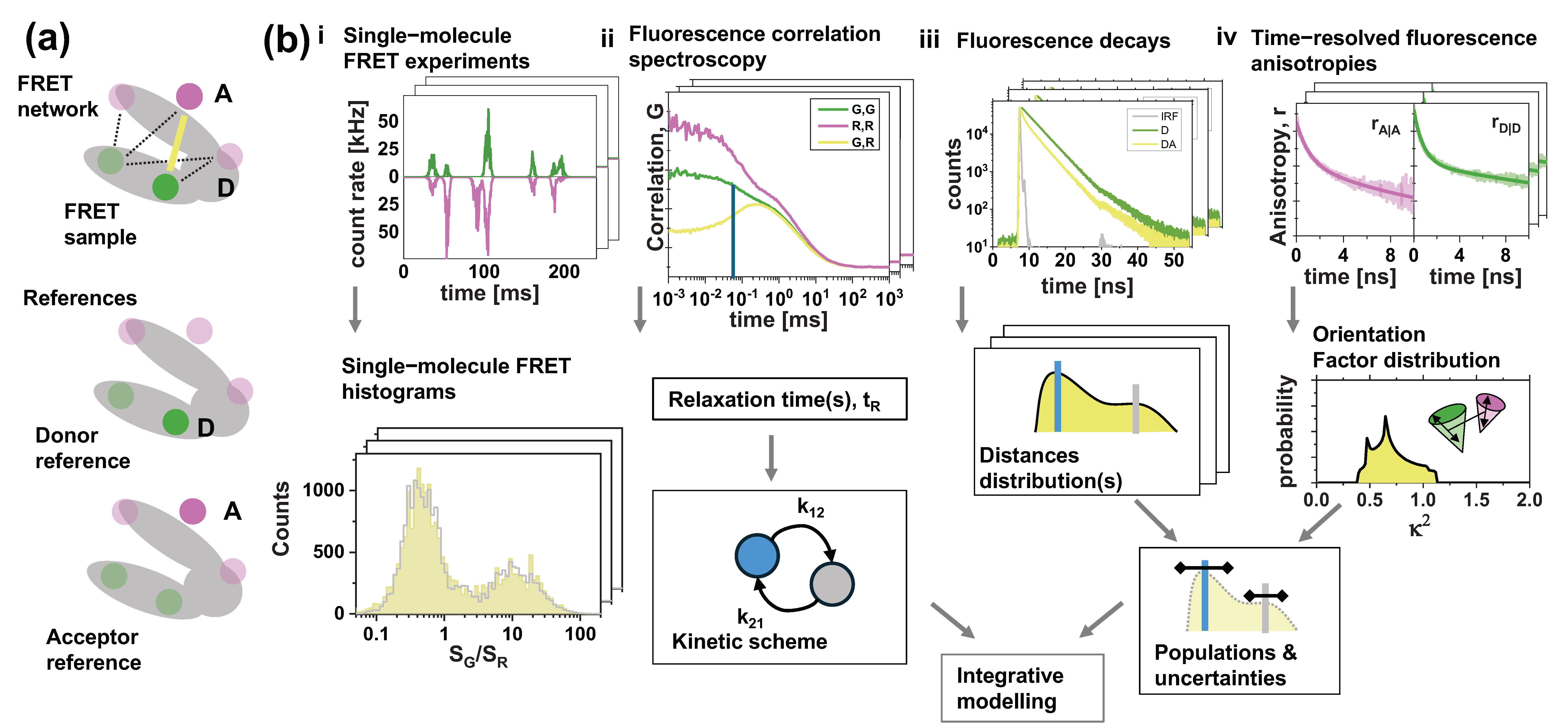
2. Materials and Methods

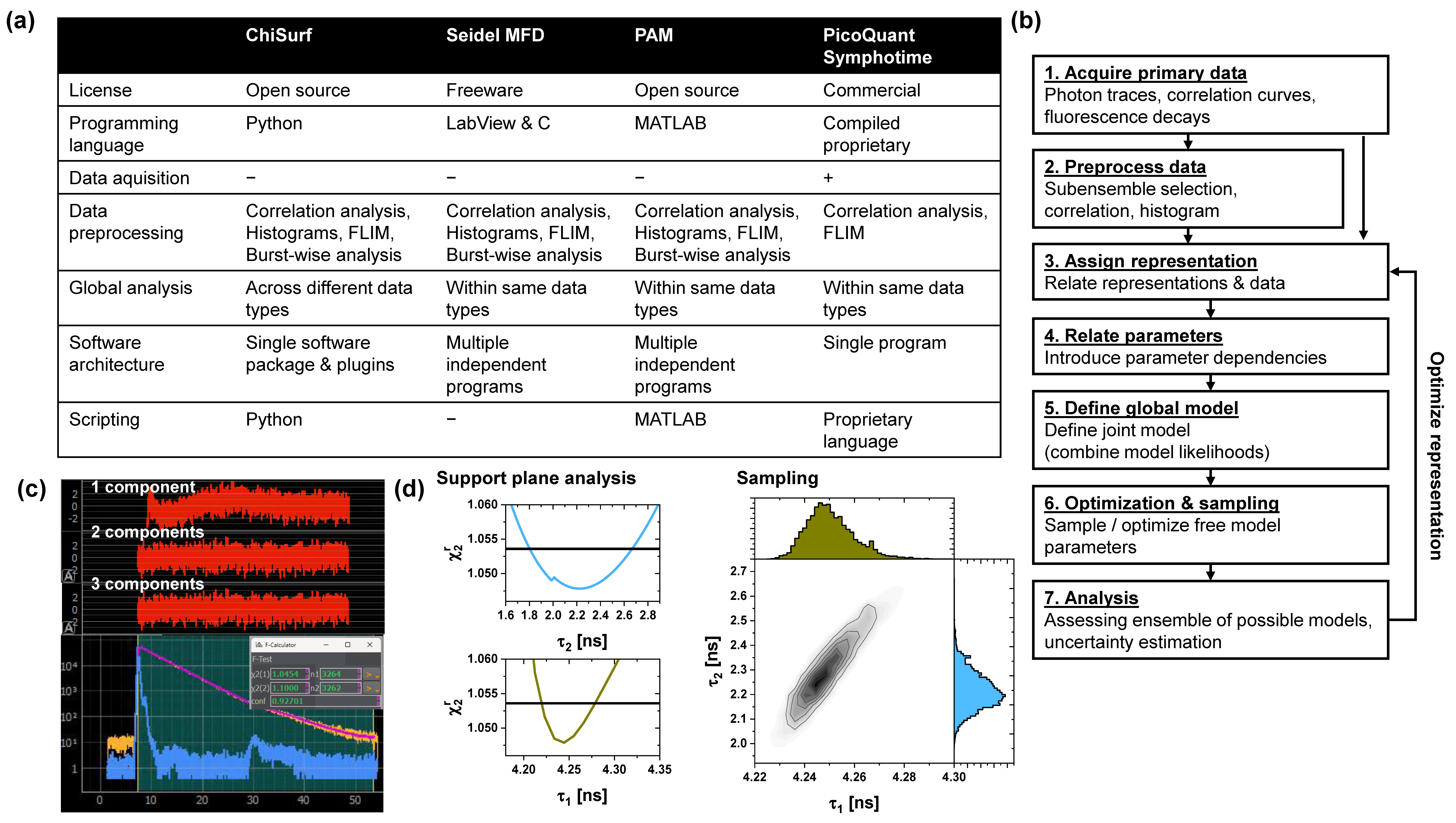
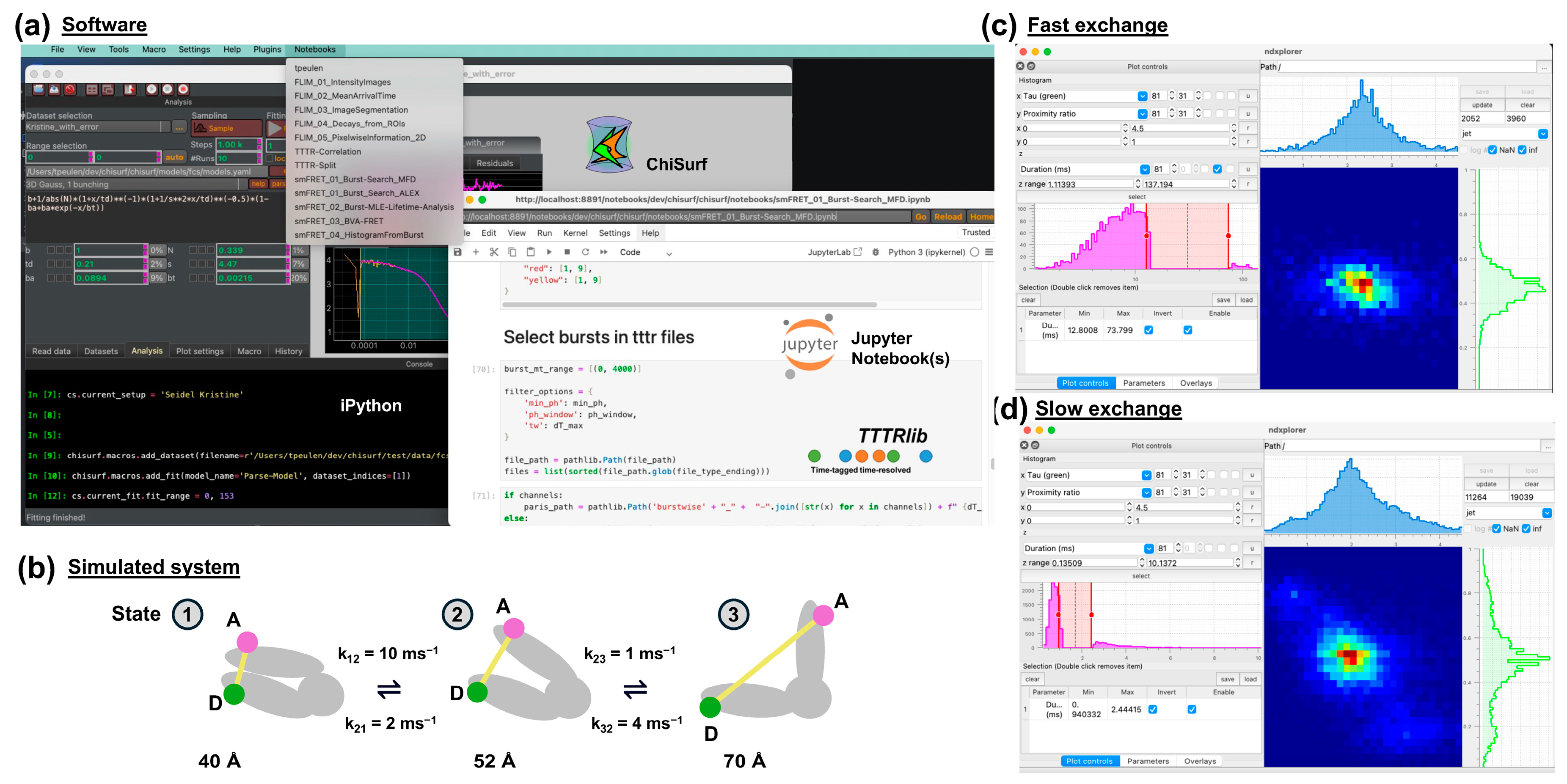
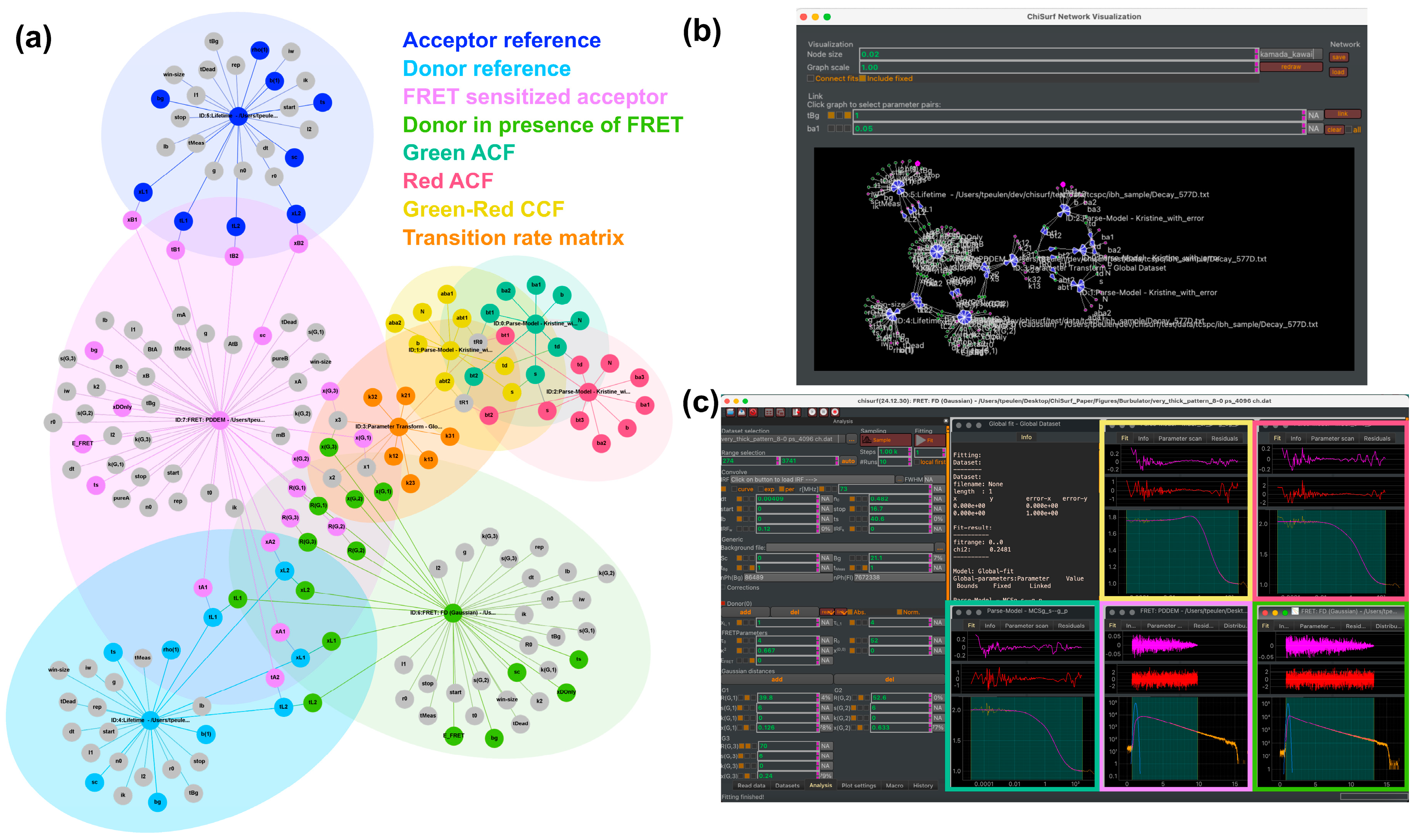
2.1. Software

ChiSurf was developed to jointly analyze multiple datasets and sample χ² surfaces and posterior model densities. It is implemented in Python 3 with a graphical user interface designed using PyQt. The software organizes data and models into “fits”, where models are equipped with parameters that can be defined as free, fixed, or linked. Linked parameters introduce dependencies between fits, enabling the grouping of individual fits into global fits. This feature allows for the analysis of complex, interconnected datasets. ChiSurf supports multiple experimental techniques, including time-correlated single-photon counting (TCSPC), fluorescence correlation spectroscopy (FCS), and single-molecule Förster resonance energy transfer (smFRET) efficiency histograms. It facilitates the combination of models from different experimental setups, allowing for comprehensive descriptions across varied experiment types. This capability is crucial for deriving meaningful insights from diverse datasets.

A flexible “adapter” system allows parameters from one component of the model—such as rate constants in a transition rate matrix—to be linked to other components. For instance, the equilibrium population of each species can be computed from the transition rate matrix and then used as the species fraction in time-correlated single-photon counting (TCSPC) experiments. Simultaneously, the eigenvalues of that same transition rate matrix define the relaxation times relevant for fluorescence correlation spectroscopy (FCS). By combining the analysis of FCS and TCSPC datasets under one unified framework, Chisurf can resolve components of the transition rate matrix more reliably than separate analyses would allow. This integrated approach ensures that both equilibrium and kinetic aspects of the system are consistently and accurately modeled, leading to more robust and comprehensive interpretations of molecular kinetics.

User interactions with the graphical user interface do not require Python scripting but directly link to commands in an embedded IPython shell. This design provides users with flexible scripting capabilities without requiring manual coding and additionally to Jupyter Notebooks, which facilitate development workflows. The open-source source code and documentation are continuously updated and freely available (https://github.com/fluorescence-tools/chisurf, https://doi.org/10.5281/zenodo.15170559). The compiled version comes with a complete Conda distribution. In addition to its core functionalities—designing models, introducing parameter dependencies, and optimizing or sampling parameters for various data types—ChiSurf ensures adaptability and robustness for advanced fluorescence data analysis.

2.2. Nomenclature

To demonstrate the software’s capabilities, we process multiparameter fluorescence detection (MFD) single-molecule and MFD image spectroscopy data. MFD setups have polarization-resolved “green” and “red” detection channels for the donor and acceptor, respectively. MFD-PIE (Pulsed Interleaved Excitation) uses two light sources, referred to as “green” and “red”, to excite the sample. This allows for assessing in FRET experiments the donor and acceptor fluorescence separately [43]. Subscripts refer to the excitation and detection of fluorescence. The subscript $\dots |G$ refers to an excitation of the sample by a “green” light source, and the subscript $\dots |R$ refers to an excitation of the sample by a “red” light source. The green detection channel is referred to by the subscript $G|\dots$. The red detection channel is referred to by the subscript $R|\dots$. The subscript “$R|G$” refers to red detection given a green excitation. Molecular species are referred to by superscripts. The superscript (DA) refers to a molecular species with a donor and an acceptor. The superscript (D0) refers to a species without an acceptor fluorophore. We distinguish the detected signal, $S$, from the background, $B$, and the fluorescence intensity, $I$:

$$S=I+B$$

(1)

Moreover, we distinguish fluorescence intensities uncorrected for spectral crosstalk and crosstalk-corrected fluorescence intensities. Fluorescence intensities corrected for crosstalk are referred to by the “dye”. In a FRET experiment on species $\left(i\right)$, $I_{D|D}^{\left(i\right)}$ and $I_{A|D}^{\left(i\right)}$ refer to the fluorescence intensity of the donor and the FRET-sensitized acceptor, respectively. $I_{D|D}^{\left(i\right)}$ and $I_{A|D}^{\left(i\right)}$ can be computed using components, ${\alpha }_{i|j}$, of the crosstalk matrix $\mathsf{\alpha }$, and components, ${\mathrm{g}}_{\mathrm{X}|\mathrm{Y}}$, of the instrumental sensitivity matrix, $\mathbf{g}$:

$$\begin{gathered} I_{D|D}^{\left(i\right)}=g_{D|G}^{-1}\left(I_{G|\mathrm{G}}^{\left(i\right)}-{\alpha }_{G|R}{I}_{\mathrm{R}|\mathrm{G}}^{\left(i\right)}\right) \\ {I}_{A|D}^{\left(i\right)}=g_{A|R}^{-1}\left(I_{R|G}^{\left(i\right)}-{\alpha }_{R|G}{I}_{\mathrm{G}|G}^{\left(i\right)}\right). \end{gathered}$$

(2)

The component ${\alpha }_{i|j}$ of the crosstalk matrix is usually determined experimentally and depends on the spectral properties of the fluorophore and experimental setup. The component $g_{X|Y}$ of the crosstalk matrix is the sensitivity of detector $Y$ for detecting the dye $X$. For instance, $g_{D|G}$ and $g_{A|R}$ are the sensitivities for detecting a donor and acceptor dye by the green and red detectors, respectively [21]. In most FRET experiments, crosstalk from A to D, ${\alpha }_{G|R}{F}_{G|R}^{\left(i\right)}$, is small. Consequently, crosstalk corrections of donor signals are often omitted. Corrections are often assumed to be identical for all conformational states [22,29,44,45]. However, users should be aware that incorrect assumptions about crosstalk corrections can lead to significant errors in quantitative FRET analysis.

In addition to the spectral features, the fluorescence quantum yield, ${\mathit{\Phi }}_X$, of the fluorophore $X$ needs to be considered to yield a fully corrected fluorescence intensity, $F_{X|\dots }$. For species $\left(i\right)$, the fluorescence intensity of the FRET-sensitized acceptor corrected for the fluorescence quantum yield is

$$F_{A|D}^{\left(i\right)}=I_{A|D}^{\left(i\right)}/{\mathit{\Phi }}_A.$$

(3)

Note that in single-molecule experiments, the excitation irradiance is usually high. Thus, the quantum yields may be lower due to populated dark states, e.g., due to cis/trans isomerization in Cy5 [46], and may require additional corrections [43,47]. Additionally, distinct species can have distinct fluorescence quantum yields. Correcting experimental data often introduces additional complexity to the noise. Therefore, in the software, corrections are implemented as model perturbations.

2.3. Förster Theory

Our software provides generic models for describing the dipolar coupling between donor, D, and acceptor, A, fluorophores to measure distances via FRET. The efficiency of the energy transfer process from a donor, D, to an acceptor, A, depends on the $k_{RET}$, the rate constants of the FRET process and $k_D$, a rate constant related to the donor’s radiative lifetime, ${\tau }_{D0}$, ($k_D=1/{\tau }_{D0}$).

$$E={\displaystyle \frac{k_{RET}}{k_D+k_{RET}}}.$$

(4)

The FRET rate constant, $k_{RET}$, depends on the inter-dye distance, $R_{DA}$. This dependence is quantitatively described by the Förster relationship,

$$k_{RET}={\kappa }^2·k_{F,D}·{\left({\displaystyle \frac{R_{0,r}}{R_{DA}}}\right)}^6.$$

(5)

Here, ${\kappa }^2$ is an orientation factor, dependent on the mutual fluorophore dipole orientation; $k_{F,D}$ is the radiative rate of the donor; and $R_{0,r}$ is the reduced dye pair Förster radius given by the refractive index, n, and the spectral overlap integral, J [48,49].

$$R_{0r}^6={\displaystyle \frac{9\ln 10}{128{\pi }^5{N}_A}}{\displaystyle \frac{J}{n^4}}.$$

(6)

Note, in this definition, the Förster radius is independent of κ² and the sample-specific donor quenching (Φ_F,D). The orientation factor κ² only appears once in the $k_{RET}$, facilitating the explicit handling of orientational effects.

Often the orientation factor ${\kappa }^2$ is assumed to be 2/3 (isotropic averaging). However, for freely rotating dyes, it is time-dependent [50]. Models that recover distances assuming 2/3 (without further evidence) recover apparent distances, $R_{app}$. The software implements different approaches for handling ${\kappa }^2$, described in more detail below (Section 2.8, Orientation Factor Distributions).

Experimentally, the efficiency of the FRET process, $E$, can be quantified by the corrected fluorescence intensities of D in the presence of A, $F_{D|D}^{\left(DA\right)}$, and the FRET-sensitized acceptor fluorescence, $F_{A|D}^{\left(DA\right)}$:

$$E={\displaystyle \frac{F_{A|D}^{\left(DA\right)}}{F_{D|D}^{\left(DA\right)}+F_{A|D}^{\left(DA\right)}}}.$$

(7)

Here, the denominator, $F_{D|D}^{\left(DA\right)}+F_{A|D}^{\left(DA\right)}$, serves as an estimate for the number of molecules in the excited donor and acceptor states, and $F_{A|D}^{\left(DA\right)}$ estimates the number of molecules that transferred energy from a donor to an acceptor due to FRET.

Alternatively, the FRET efficiency can be estimated by the change in the donor fluorescence intensity in the absence, $F_{D|D}^{\left(D0\right)}$, and presence of an acceptor, $F_{A|D}^{\left(DA\right)}$.

$$E={\displaystyle \frac{F_{D|D}^{\left(D0\right)}-F_{D|A}^{\left(DA\right)}}{F_{D|D}^{\left(D0\right)}}}.$$

(8)

Likewise, the FRET efficiency can be measured by changes in the donor’s fluorescence lifetime:

$$E={\displaystyle \frac{{\tau }_{D0}-{\tau }_{DA}}{{\tau }_{D0}}}.$$

(9)

For a homogenous sample with a single FRET rate constant, $k_{RET}$, and a single fluorescence lifetime of the donor in the absence of FRET, ${\tau }_{D0},$ estimating $E$ via Equations (7)–(9) allows us to determine distances via the FRET (Equation (5)).

2.4. Time-Resolved Experiments

Our software supports FRET analysis of time-resolved fluorescence decays, $f\left(t\right)$. Fluorescence decays are proportional to the population of the excited state, $p\left(t\right)$, and the radiative rate of the emitting fluorophore, $k_F$. An analysis of $f\left(t\right)$ allows us to resolve distances and sample heterogeneities.

The simplest case involves the joint analysis of fluorescence decays in the absence and presence of FRET. Generally, time-resolved FRET measurements require no instrumental intensity calibration. They measure the excited-state lifetime of the donor in the presence of FRET, ${\tau }_{DA}^{\left(i\right)}={\left(k_D+k_{RET}^{\left(i\right)}\right)}^{-1}$. Briefly, FRET rate constants are obtained by a global description of the donor’s excited-state population in the absence, $p_{D|D}^{\left(D0\right)}$, and in the presence, $p_{D|D}^{\left(DA\right)}$, of FRET:

$$\begin{gathered} p_{D|D}^{\left(D0\right)}=e^{-k_D·t} \\ {p}_{D|D}^{\left(DA\right)}=e^{-k_D·t}·e^{-k_{RET}·t} \\ {p}_{A|D}^{\left(AD\right)}={\displaystyle \frac{k_{RET}}{k_A-k_D-k_{RET}}}·(e^{-k_D·t}·e^{-k_{RET}·t}-e^{-k_A·t}) \end{gathered}$$

(10)

Here, $p_{D|D}^{\left(DA\right)}$ can be factorized into ${ϵ}_D\left(t\right)$, the time-dependent depopulation of the donor (FRET-induced donor decay), and $p_{D|D}^{\left(D0\right)}$. A more detailed description and an extension to Partial Donor–Donor Energy Migration (PDDEM), which served as the basis for the software implementation, can be found in Kalinin et al. [51].

Such factorizing has been shown to be accurate for multiexponential $f_{D|D}^{\left(D0\right)}$ if FRET and other quenching processes are uncorrelated [21]. The FRET-induced donor decay depends on $R_{DA}$ and ${\kappa }^2$:

$${ϵ}_D\left(t\right)=\int \int p\left({\kappa }^2,R_{DA},t\right)e^{-t·{\displaystyle \frac{3}{2}}·{\kappa }^2·{\displaystyle \frac{1}{{\tau }_{F,D}}}{\left({\displaystyle \frac{R_{0,r}}{R_{DA}}}\right)}^6}d{R}_{DA}d{\kappa }^2.$$

(11)

Above, $p\left({\kappa }^2,R_{DA},t\right)$ is a time-dependent distribution. It is difficult to disentangle $p\left({\kappa }^2,R_{DA},t\right)$ to obtain a distance distribution, $p\left(R_{DA}\right)$. Four common approximations help in determining $p\left(R_{DA}\right)$: (i) ${\kappa }^2$ and $R_{DA}$ are independent; (ii) $p\left({\kappa }^2\right)$ is known (often assumed isotropic); (iii) dipoles are assumed to either rotate very fast or slow to eliminate the ${\kappa }^2$ time-dependence; and (iv) a reduced set of parameters is used to describe $p\left(R_{DA}\right)$, e.g., the mean and variance of normal distribution.

For independent ${\kappa }^2$ and $R_{DA}$,

$$p\left({\kappa }^2,R_{DA}\right)=p\left({\kappa }^2\right)·p\left(R_{DA}\right)$$

(12)

When molecular simulations are used to sample the orientation factor distribution in a sterically confined space, a simulated orientation factor distribution can be used for $p\left({\kappa }^2\right)$ [52]. Alternatively, $p\left({\kappa }^2\right)$ can be simulated based on experimental anisotropies, e.g., using the diffusion in a cone model. Both approaches are implemented in our analysis software. For fast-rotating dipoles (small fluorophores) compared to $k_{RET}$, the orientation factor distribution is approximated by an average $〈{\kappa }^2〉$.

$${ϵ}_{D,{\kappa }_{dyn}^2}\left(t\right)=\int p\left(R_{DA}\right)e^{-t·{\displaystyle \frac{3}{2}}·〈{\kappa }^2〉·{\displaystyle \frac{1}{{\tau }_{F,D}}}{\left({\displaystyle \frac{R_{0,r}}{R_{DA}}}\right)}^6}d{R}_{DA}$$

(13)

Here, ${ϵ}_{D,{\kappa }_{dyn}^2}$ is the FRET-induced donor decay for fast-rotating dipoles. Dipoles that rotate slowly compared to $k_{RET}$ (for instance fluorescent proteins (FPs)) are better described by a static p(κ2):

$${ϵ}_{D,{\kappa }_{static}^2}\left(t\right)=\int \int p\left({\kappa }^2\left)p\right(R_{DA}\right)e^{-t·{\displaystyle \frac{3}{2}}·{\kappa }^2·{\displaystyle \frac{1}{{\tau }_{F,D}}}{\left({\displaystyle \frac{R_{0,r}}{R_{DA}}}\right)}^6}d{R}_{DA}d{\kappa }^2$$

(14)

Here, ${ϵ}_{D,{\kappa }_{static}^2}$ is the FRET-induced donor decay of static dipoles, i.e., dipoles that rotate slowly compared to their fluorescence lifetime. The latter approximation applies to FPs that slow (~16 ns) compared to their fluorescence lifetime (~2.6 ns) [53]. Intermediate cases can be modeled using simulations [50]. Similar considerations regarding the averaging regimes apply to the inter-dye distance. For small organic fluorophores, we recovered correct distance distributions using a static orientation model even though there is considerable displacement of the dyes on the timescale of FRET [21].

Inter-dye distributions, $p\left(R_{DA}\right)$, can be approximated by a linear combination of normal distributions:

$$p(R_{DA};{\sigma }_{DA}, \overline{R_{DA}})={\displaystyle \frac{1}{2\pi {\sigma }_{DA}^2}}{e}^{-{\displaystyle \frac{1}{2}}{\left({\displaystyle \frac{R_{DA}-\overline{R_{DA}}}{{\sigma }_{DA}}}\right)}^2}$$

(15)

where ${\sigma }_{DA}$ and $\overline{R_{DA}}$ are the width and the center of the inter-dye distance distribution, respectively. Alternatively, $p\left(R_{DA}\right)$ is described by a linear combination of chi distributions:

$$p\left(R_{DA};{\sigma }_{dye}, R_{cc}\right)={\displaystyle \frac{R_{DA}}{R_{cc}}}·(N\left(R_{DA}|{\sigma }_{dye},R_{cc}\right)-N\left(R_{DA}|{\sigma }_{dye},-R_{cc}\right))$$

(16)

Here, ${\sigma }_{dye}$ is the width of the spatial dye distribution, and $R_{cc}$ is the center-to-center distance between the two dyes. Such a description is accurate for flexible tethered dyes [29] but also applies to fluorescent proteins coupled via unstructured and flexible amino acids at the N- and C-termini [30,40].

In practice, experimental nuisances, e.g., convolutions with the instrument response function, IRF, the background, and the anisotropy of the dyes, need to be considered to recover $p\left(R_{DA}\right)$ parameters. Our software allows for a joint analysis of $f_{G|G}^{\left(D0\right)}\left(t\right)$ and $f_{G|G}^{\left(DA\right)}\left(t\right)$, the FRET-sensitized acceptor decay $f_{R|G}^{\left(DA\right)}\left(t\right)$, and the acceptor directly excited by a “red” light source, $f_{R|R}^{\left(DA\right)}\left(t\right)$. In DA, D0, and A0 species mixtures, the registered fluorescence decay $f_{G|G}^{\left(mix\right)}$ is a species fraction and an excitation and detection probabilities-weighted combination of $f_{D|D}^{\left(DA\right)}$, $f_{D|G}^{\left(D0\right)}, f_{A|G}^{\left(DA\right)}$, and $f_{A|A}^{\left(A0\right)}$.

Time-Resolved Anisotropy

Fluorescence generally leads to signal depolarization. The extent of this effect is described by a property called anisotropy, $r$. Molecular motions on the timescale of the fluorescence lifetime affect the shape of the fluorescence intensity decays unless detection is performed under magic-angle conditions. By measuring the parallel, $f_{||}\left(t\right),$ and the perpendicularly polarized component, $f_{\perp }\left(t\right)$, of the fluorescence decay, the anisotropy decay r(t) can be determined. The parallel component $f_{||}\left(t\right)$ is

$$f_{||}\left(t\right)={\displaystyle \frac{1}{3}}·f\left(t\right)·\left(1+2r\left(t\right)\right)$$

(17)

whereas the perpendicularly polarized component $f_{\perp }\left(t\right)$ is corrected by $G$, an experimental factor correcting for the relative sensitivity of the parallel/perpendicular detector.

$$f_{\perp }\left(t\right)/G={\displaystyle \frac{1}{3}}·f\left(t\right)·\left(1-r\left(t\right)\right)$$

(18)

Note that in a microscope with a high numerical aperture (NA), an additional correction for mixing of the parallel and perpendicular light is needed [54,55]. Both layers of corrections are implemented in our software.

A typical anisotropy decay is modeled as a multiexponential function, such as

$$r\left(t\right)={\sum }_k{b}^{\left(k\right)}\exp \left(-{\displaystyle \frac{t}{{\rho }^{\left(k\right)}}}\right).$$

(19)

Here, $r_0={\sum }_k{b}_i^{\left(k\right)}$ is the fundamental anisotropy of the molecule. Being dependent on the fluorescence lifetime, the anisotropy r can also be used as an indicator for FRET and for quantitative FRET measurements [56].

Besides rotational motions and lifetime changes, fluorescence depolarization can also be caused by energy transfer between chemically identical fluorophores. Homotransfer is also described by Förster’s theory—i.e., the dependence of transfer efficiency on the distance—but does not change the observed intensity decays, making anisotropy the only observable for this process. HomoFRET (Förster Resonance Energy Transfer between identical fluorophores) is commonly used to study protein interactions in situ by polarization microscopy [57,58,59], having the advantage of relative simplicity of labeling (one type of dye) and instrumentation (only polarization or polarization and frequency-domain FLIM). HeteroFRET (FRET between different donor and acceptor fluorophores) has the advantage of more observables—such as donor/acceptor intensity ratios and fluorescence lifetime—offering better distance resolution and greater flexibility for controlling experiment conditions.

To recover precise distances, our software includes comprehensive models for analyzing $f_{D|D}^{\left(DA\right)}$, $f_{D|G}^{\left(D0\right)}, f_{A|G}^{\left(DA\right)}$, and $f_{A|A}^{\left(A0\right)}$, incorporating corrections for nuisance parameters such as scattered light, background noise, time shifts, and FRET-inactive species. These nuisance parameters are essential for addressing experimental artifacts that can distort the data, ensuring accurate recovery of distance and rate parameters. For example, background noise and scattered light can introduce spurious signals, while time shifts may cause discrepancies in decay measurements. Accounting for FRET-inactive species helps isolate signals from active donor–acceptor pairs, reducing bias and improving model accuracy. In addition to classic FRET models, the software implements the Partial Donor–Donor Energy Migration model (PDDEM) [60], which accounts for forward and backward energy transfer. Sampling across model parameters allows for error estimation, enabling reliable distance measurements and integrative modeling for structural determination. All routines and models are accessible interactively through the graphical user interface (GUI) or via scripting.

2.5. Burst Analysis

Our software can process data from single-molecule confocal experiments. In such experiments, single molecules are detected during their free diffusion through a confocal volume. The resulting photon bursts are selected from the recorded photon trace after background separation. This is accomplished by applying a threshold for the maximum inter-photon time and a minimum photon number within a burst (typically 30–160 photons) [61]. The burst duration is determined mainly by the experimental setup and the molecular dimensions. As the molecules are freely diffusing, a distribution of burst durations is observed, and the fluorescence observables are averaged according to the individual burst durations. Due to the low number of photons (60–500 photons per burst) detected per burst, it is not practical to apply complex models to describe the fluorescence intensity decays [62].

To process such data, ChiSurf provides Jupyter Notebooks for burst selection [61], and burst-wise fluorescence lifetime analysis using maximum likelihood estimation (MLE) algorithms [62] and anisotropy analysis [63]. For each burst, intensity-based parameters (e.g., green and red count rates for green and red excitation) and anisotropy-based parameters (e.g., the number of photons in parallel and perpendicular polarizations) are determined, allowing for the construction of multidimensional frequency histograms. Burst selection and sub-ensemble analyses are conducted using NDxplorer, a module of ChiSurf specifically designed for creating and analyzing n-dimensional single-molecule histograms and exporting burst selections as sub-ensembles.

2.6. Single-Molecule Histograms

Single-molecule histograms computed for the signal detected by two distinct detectors are widely used to analyze single-molecule traces and determine distances via FRET or anisotropy, particularly in confocal microscopy data. The simplest way to analyze these histograms is by fitting a sum of normal distributions to recover the means of the underlying populations [64,65]. However, the fitted width of populations using traditional methods has no physical meaning (as it is a combination of physical width and shot noise), overlapping states cannot be accurately resolved, and minor states may be overlooked. Furthermore, without proper weighting of the residuals, the quality of the fit cannot be reliably assessed. These complications have been overcome by Photon Distribution Analysis (PDA) and related methods [24,39,66,67,68,69].

Our software focuses on analyzing confocal-derived FRET histograms by using Photon Distribution Analysis (PDA), an approach that accounts for shot noise and Poisson photon statistics to provide more accurate insights into FRET efficiencies, rate constants, and population fractions. PDA overcomes the limitations of traditional methods, ensuring a precise representation of the underlying populations [45,66,70,71,72]. We implemented a generic PDA framework that can be used to analyze both anisotropy and FRET data [24,39]. The framework accounts for Poisson statistics of the photon distribution and broadening caused by shot noise.

PDA is accomplished by calculating the probability $P(S_G, S_R)$ of observing a certain combination of photons collected in the “green” (G) and “red” (R) detection channels:

$$P\left(S_G, S_R\right)={\sum }_{F_G+B_G=S_G;F_R+B_R=S_R}P\left(F\right)P(F_G,F_R|F\left)P\right(B_G\left)P\right(B_R).$$

(20)

The software implements a previously proposed deconvolution method to recover the distribution of fluorescence signals from the observed photon count distribution using the known background count distribution [68]. This approach is available through the PDA implementation of tttrlib [73]. However, it is not yet accessible via the graphical user interface (GUI).

Assuming that the background signals $B_G$ and $B_R$ are distributed according to Poisson distributions, the fluorescence intensity distribution, $P\left(F\right)$, can be obtained from the total signal intensity distribution, $P\left(S\right)$, using the known background count distributions, P(B_G) and P(B_R), with mean intensities $B_G$ and $B_R$. The conditional probability $P(F_G,F_R|F)$ represents the probability of observing a particular combination of green and red fluorescence photons, $F_G$ and $F_R$, given that the total number of registered fluorescence photons is $F$. This probability follows a binomial distribution [39]:

$$P\left(F_G,F_R|F\right)={\displaystyle \frac{F!}{F_G!\left(F-F_G\right)!}}{p}_G^{F_G}{\left(1-p_G\right)}^{F-F_G}.$$

(21)

Here, $p_G$ is the probability a detected photon is registered in the “green” detection channel. In a FRET experiment, the probability $p_G$ is unambiguously related to the FRET efficiency $E$:

$$p_G={\left(1-{\alpha }_{R|G}+\gamma ·{\displaystyle \frac{E}{1-E}}\right)}^{-1}.$$

(22)

where $\gamma =\left({\mathrm{\Phi }}_A{g}_{A|R}\right)/\left({\mathrm{\Phi }}_D{g}_{D|G}\right)$ and ${\alpha }_{R|G}$ is the crosstalk from the G to the R channel. Knowledge of $P(S_G, S_R)$ is sufficient to compute 1D histograms of any FRET-related parameter, which can be expressed as a function of $S_G$ and $S_R$ (e.g., signal ratio $S_G/S_R$ or FRET efficiency $E$) [24]. Fitting such histograms obtained for a single species requires only one free parameter, $p_G$.

In PDA, intensities are averaged on the millisecond timescale. Hence, a determined distance, $R_E$, is an average distance, and the distribution width carries limited information for fast dynamic systems. Moreover, a varying acceptor quantum yield, ${\mathrm{\Phi }}_{F,A}^{\left(A0\right)}$, results in broadening of the observed FRET distributions beyond the shot noise [70]. Thus, complex model functions are often necessary to describe experimental data. In practice, broadening associated with ${\mathrm{\Phi }}_{F,A}^{\left(A0\right)}$ is well approximated by Gaussian distance distributions [74]. Additionally, in anisotropy experiments, the “green” and “red” detectors correspond to parallel and perpendicular detectors. Instead of $p_G$ (relating FRET efficiency and photon detection probability in the green channel), the anisotropy model is used [24].

To account for more complex cases, our software separates PDA histogram computation of raw signals from derived parameters such as FRET efficiency and anisotropy histograms. This modularization enables flexible analysis of various experimental relations and setups, supporting global fits with customizable models based on distributions of $p_G$. By decoupling raw signal processing from parameter derivation, the software allows us to incorporate models via Python scripting. While Python scripting provides maximum flexibility—allowing users to define custom parameter transforms and implement sophisticated models—it requires basic programming skills. In contrast, the GUI offers an intuitive approach for standard analyses without requiring coding but is less adaptable. Decorated Python functions facilitate the generation of parameter transforms, converting PDA histograms into new or different representations. This flexibility enables users to tailor the analysis to specific experimental needs, but those unfamiliar with scripting may prefer to rely on the GUI for predefined models.

2.7. Fluorescence Correlation Spectroscopy

Our software supports fluorescence correlation spectroscopy (FCS) [75,76,77]. FCS, in combination with FRET (FRET-FCS), was developed as a powerful tool [78,79] to study fluctuations in the time evolution of a signal distance change. FRET-FCS allows for the analysis of FRET fluctuations covering a time range from nanoseconds to seconds. Hence, it is an ideal method for studying conformational dynamics of biomolecules, complex formation, folding, and catalysis [78,79,80,81,82,83,84,85,86]. Structural fluctuations are reflected in the correlation function, which in turn provides restraints on the number of conformational states. In this section, we briefly describe the simplest case of FRET-FCS and discuss various experimental scenarios [27].

Briefly, the auto/cross-correlation of two correlation channels, $S_A$ and $S_B$, is given by

$$G_{A,B}\left(t_c\right)=1+{\displaystyle \frac{⟨\delta S_A\left(t\right)·\delta S_B\left(t+t_c\right)⟩}{⟨S_A\left(t\right)⟩⟨S_B\left(t\right)⟩}}.$$

(23)

If $S_A$ equals $S_B$, the correlation function is called an autocorrelation function (ACF); otherwise, it is a cross-correlation function (CCF). ACFs and CCFs can be analyzed to provide insights into kinetics, the number of molecules, and species populations [13,37]. If all species have equal brightness, the amplitude at zero time of the autocorrelation function, G(0), allows for the determination of the mean number of molecules N in the detection volume:

$$G\left(t_c=0\right)=1+{\displaystyle \frac{1}{N}}·G_{diff}\left(t_c\right).$$

(24)

For a three-dimensional (3D) Gaussian-shaped detection/illumination volume, the normalized diffusion term, $G_{diff}$, is given by

$$G_{diff}\left(t_c\right)={\left(1+{\displaystyle \frac{t_c}{t_{diff}}}\right)}^{-1}·{\left(1+{\left({\displaystyle \frac{{\omega }_0}{z_0}}\right)}^2·{\displaystyle \frac{t_c}{t_{diff}}}\right)}^{-{\displaystyle \frac{1}{2}}}$$

(25)

where ${\omega }_0$ and $z_0$ are shape parameters of the detection volume $w\left(x,y,z\right)=\exp \left(-2\left(x^2+y^2\right)/{\omega }_0^2\right)\exp (-2z^2/z_0)$. $G_{diff}\left(t_c\right)$ allows for a direct assessment of the diffusion coefficient, D_diff (in one-photon excitation: $t_{diff}={\omega }_0^2/\left(4D_{diff}\right)$).

In the simplest case of a two-state system with different FRET levels and exchange rate constants, $k_{12}$ and $k_{21}$, and comparable diffusion coefficients, in the sole presence of DA-molecules and in the absence of bleaching ($G_{GR}=G_{RG}$) and dark states (e.g., triplet states), the ACFs and the CCF have a simple analytical solution:

$$\begin{gathered} G_{GG}\left(t_c\right)=1+{\displaystyle \frac{1}{N}}·G_{diff}\left(t_c\right)·\left[1+A{C}_{GG}·\exp \left(-{\displaystyle \frac{t_c}{t_R}}\right)\right] \\ {G}_{RR}\left(t_c\right)=1+{\displaystyle \frac{1}{N}}·G_{diff}\left(t_c\right)·\left[1+A{C}_{RR}·\exp \left(-{\displaystyle \frac{t_c}{t_R}}\right)\right] \\ {G}_{GR}\left(t_c\right)=1+{\displaystyle \frac{1}{N}}·G_{diff}\left(t_c\right)·\left[1-{\left(A{C}_{GG}·A{C}_{RR}\right)}^{1/2}·\exp \left(-{\displaystyle \frac{t_c}{t_R}}\right)\right] \end{gathered}$$

(26)

Here, $A{C}_{GG}$, $A{C}_{RR}$, and $A{C}_{GR}$ are the amplitudes of the kinetic reaction terms, and $t_R$ is a relaxation time related to the exchange rate constants ($t_R={(k_{12}+k_{21})}^{-1}$)). The amplitudes depend on the molecular brightnesses, an intrinsic molecular property of the dyes and the FRET states [87]. The molecular brightness of species $i$ is proportional to the product of the focal excitation irradiance, $I_0$, the extinction coefficient, ${ϵ}^{\left(i\right)}$, the fluorescence quantum yield, ${\mathrm{\Phi }}_F^{\left(i\right)}$, and detection efficiencies $g_G^{\left(i\right)}$ or $g_R^{\left(i\right)}$ for green and red detectors for species $i$, respectively ($Q_{G,R}^{\left(\mathrm{i}\right)}\propto I_0{ϵ}^{\left(i\right)}{\mathrm{\Phi }}_F^{\left(i\right)}{g}_{G,R}^{\left(i\right)}$) [61,88]. The molecular brightness corresponds to the observed photon count rate per molecule, $Q^{\left(i\right)}=F^{\left(i\right)}/N^{\left(i\right)}$, where $F^{\left(i\right)}$ is the total number of fluorescence photons of $N^{\left(i\right)}$ molecules of species i. In the presence of FRET, $Q^{\left(i\right)}$ depends on the FRET efficiency, $E^{\left(i\right)}$, of the species $i$. The brightness and the FRET efficiencies are often unknown in practice. Hence, $A{C}_{GG}$, $A{C}_{RR}$, and $A{C}_{GR}$ are treated as variable parameters.

Our software provides Jupyter Notebooks for the computation of correlation functions, allowing the implementation of advanced correlation techniques that enhance the contrast. For example, fluorescence lifetime [89] can be utilized to distinguish molecular species based on their specific fluorescence lifetime, polarization, and spectrally resolved fluorescence decays [90]. The framework features a flexible “adapter” system, which allows parameters—such as rate constants in a transition rate matrix—to be linked to other model components, such as relaxation times. Such a setup can be integrated within a theoretical framework for multistate systems [13,37].

2.8. Orientation Factor Distributions

To determine accurate distances from FRET measurements, we implemented methods for assessing ${\kappa }^2$ uncertainties, as ${\kappa }^2$-error gathers most of the attention. For small dyes, the dye reorientation dynamics is on the timescale of FRET [60] and could be relevant for very short distances and dyes attached with short linkers [29,91,92]. For large fluorophores (e.g., fluorescent proteins), the fluorophore rotation is slow ($\approx 16 \mathrm{n}\mathrm{s}$) compared to the fluorescence lifetime ($\approx 2.3 \mathrm{n}\mathrm{s}$) [53]. Without molecular simulations, the mutual fluorophore orientation is unknown. Thus, assuming an isotopic dipole orientation is reasonable. For isotropically oriented dipoles, the orientation factor distribution is

$$p({\kappa }^2)=\left\{\begin{array}{ll}{\displaystyle \frac{1}{2\sqrt{3{\kappa }^2}}}\ln \left(2+\sqrt{3}\right)& 0\le {\kappa }^2\le 1\\ {\displaystyle \frac{1}{2\sqrt{3{\kappa }^2}}}\ln \left({\displaystyle \frac{2+\sqrt{3}}{\sqrt{{\kappa }^2}+\sqrt{{\kappa }^2-1}}}\right)& 1\le {\kappa }^2\le 4\end{array}\right..$$

(27)

For a single DA distance, $R_{DA}$, a single FRET rate constant, $k_{RET}$, is observed if the fluorophores rotate fast compared to the fluorescence lifetime. In this case, $p\left({\kappa }^2\right)$ can be replaced by its average value $⟨{\kappa }^2⟩=2/3$ (dynamic average). If the fluorophores rotate slowly compared to the fluorescence lifetime, then for a single $R_{DA}$, a distribution of FRET rate constants, $p(k_{RET}$), will be observed (static average). In both cases, $p(k_{RET}$) can be computed using $p\left({\kappa }^2\right)$.

For small, fast-rotating dyes, it was demonstrated how to experimentally test whether the assumption for 〈${\kappa }^2$〉 ≅ 2/3 is justifiable [29]. For a given model of the fluorophores—e.g., the “wobble in a cone” (WIC) model [91]—it is possible to calculate a distribution of all possible values of ${\kappa }^2$ consistent with experimental data. In the WIC model, ${\kappa }^2$ follows

$$\begin{gathered} {\kappa }^2={\displaystyle \frac{2}{3}}+{\displaystyle \frac{2}{3}}{S}_D^{\left(2\right)}{S}^{\left(2\right)}\left({\beta }_1\right)+{\displaystyle \frac{2}{3}}{S}_A^{\left(2\right)}{S}^{\left(2\right)}\left({\beta }_2\right)+{\displaystyle \frac{2}{3}}{S}_D^{\left(2\right)}{S}_A^{\left(2\right)}[S^{\left(2\right)}\left(\delta \right)+ \\ 6S^{\left(2\right)}\left({\beta }_1\right)S^{\left(2\right)}\left({\beta }_2\right)+1+2S^{\left(2\right)}\left({\beta }_1\right)+2S^{\left(2\right)}\left({\beta }_2\right)-9\cos {\beta }_1\cos {\beta }_2\cos \delta ]. \end{gathered}$$

(28)

Here, ${\beta }_1$ and ${\beta }_2$ are the angles between the symmetry axes of the dye’s rotations and the distance vector R_DA, while $\delta$ is the angle between the dye cone symmetry axis (see Supplementary Figure S1). A donor that is oriented approximately perpendicular to the linker axis is restricted to the half angle of a “disk”, ${\theta }_{disk}={\theta }_D$. This is the case for fluorophore Alexa488. Alternatively, the dipole moment oriented along the linker axis can wobble with the opening half angle ${\theta }_{cone}={\theta }_A$. This is approximately the case for Cy5 and Alexa647. For such a geometry, the second-rank order parameters $S^{\left(2\right)}$ are given by

$$\begin{gathered} S^{\left(2\right)}\left(\delta \right)={\displaystyle \frac{1}{2}}\left(3{\cos }^2\delta -1\right), \\ {S}^{\left(2\right)}\left({\beta }_1\right)={\displaystyle \frac{1}{2}}\left(3{\cos }^2{\beta }_1-1\right), \\ {S}^{\left(2\right)}\left({\beta }_2\right)={\displaystyle \frac{1}{2}}\left(3{\cos }^2{\beta }_2-1\right), \\ {S}_D^{\left(2\right)}=-{\displaystyle \frac{1}{2}}{\cos }^2{\theta }_{disk}, \mathrm{and} \\ {S}_A^{\left(2\right)}={\displaystyle \frac{1}{2}}\cos {\theta }_{cone}(1+\cos {\theta }_{cone}). \end{gathered}$$

(29)

Only a subset of all dye orientations is possible for a given combination of residual anisotropy of the donor, $r_{\infty ,D|D}$, the directly excited acceptor, $r_{\infty ,A|A}$, and the FRET-sensitized acceptor, $r_{\infty ,A|D}^{\left(DA\right)}$. This restricts the possible angles between donor and acceptor motions. The second-rank order parameters $S^{\left(2\right)}$ relate to residual anisotropies as follows:

$$\begin{gathered} -S_D^{\left(2\right)}=\sqrt{{\displaystyle \frac{r_{\infty ,D|D}}{r_0}}}, \\ {S}_A^{\left(2\right)}=\sqrt{{\displaystyle \frac{r_{\infty ,A|A}}{r_0}}}, \mathrm{and} \\ {S}^{\left(2\right)}\left(\delta \right)={\displaystyle \frac{1}{r_0}}{\displaystyle \frac{r_{\infty ,A|D}^{\left(DA\right)}}{S_D^{\left(2\right)}{S}_A^{\left(2\right)}}}. \end{gathered}$$

(30)

Thus, anisotropy decays provide useful information for determining local and global motions of dyes, as only certain $p\left({\kappa }^2\right)$ values are consistent with the dye rotation model. Note that ${\kappa }^2$ does not explicitly depend on the cone opening half-angles ${\theta }_D$ and ${\theta }_A$, and the assumption of dye reorientation within a cone/disk is not required to obtain all possible values of ${\kappa }^2$. However, axially symmetric transition dipole orientation distributions are usually a good approximation for ${\kappa }^2$ [91]. In most recent studies, ${⟨\kappa ⟩}^2$ values are ~2/3, justifying isotropic averaging of dipoles and demonstrating that the common misconception of FRET as inaccurate is not well founded. However, one cannot neglect the specific effects of the microenvironment [93,94,95], especially if slow exchange is expected.

2.9. Simulation of Synthetic Data

In real experiments, photon traces are inherently complex due to various factors, such as donor–acceptor (DA) distance distributions, brightness variations caused by the confocal excitation profile, and experimental artifacts like the instrumental response function and detector dark counts. These complexities were reproduced in simulations of freely diffusing molecules to generate realistic synthetic data. Detailed technical information on the simulations is provided in [90]. As in actual single-photon counting experiments, Poissonian statistics dictate the experimental noise and the resulting statistical uncertainties in subsequent analyses. The simulated test case aims to evaluate whether data of typical experimental quality can accurately recover distances and assess the limitations affecting their precision.

Here, we implemented a simulation of a three-state system consisting of putative states ($C_1$, $C_2$, $C_3$) undergoing a linear exchange. Thus, in our simulations, the transition rate matrix is given by

$${\displaystyle \frac{\mathrm{d}}{\mathrm{d}\mathrm{t}}}\left[\begin{array}{c}{x}^{\left(1\right)}\\ x^{\left(2\right)}\\ x^{\left(3\right)}\end{array}\right]=\left[\begin{array}{ccc}-\left(k_{21}+k_{31}\right)& k_{12}& k_{13}\\ k_{21}& -\left(k_{12}+k_{32}\right)& k_{23}\\ k_{31}& k_{32}& -\left(k_{13}+k_{23}\right)\end{array}\right]\left[\begin{array}{c}{x}^{\left(1\right)}\\ x^{\left(2\right)}\\ x^{\left(3\right)}\end{array}\right]$$

(31)

where $k_{13}=k_{31}=0$. Brownian dynamics (BD) simulations were used to mimic the statistics of typical single-molecule FRET (smFRET) experiments over a 1.5 h measurement period. In the simulations, the rate constants with a slow exchange between $C_1$ and $C_2$ ($k_{12}$ = 10 ms⁻¹, $k_{21}$ = 2 ms⁻¹) and a fast exchange between $C_2$ and $C_3$ ($k_{23}=1$ ms⁻¹, $k_{32}=4$ ms⁻¹) result in a fast ($t_{R,1}=0.0815$ ms) and a slow ($t_{R,2}=0.212$ ms) relaxation time. Simulated experiments can be reproduced using the simulation software, and the simulation settings are accessible through the ModelArchive (https://www.modelarchive.org/doi/10.5452/ma-a2hbq) and Zenodo (DOI: 10.5281/zenodo.14636405), respectively.

2.10. FLIM Experiments

2.10.1. Sample Preparation

Measurements were performed in mouse embryonic fibroblast (MEF) murine guanylate-binding protein 7 (mGBP7)-deficient cells stably transduced with eGFP-mGBP7 and mCherry-mGBP3. Generation, culture conditions, and characterization of the cell line are described in [30,96]. MEF cells were seeded in fully supplemented DMEM medium and grown until 70–80% confluence in Nunc™ LabTek™ II 8-well chambers (ThermoFisher). For live-cell pulsed interleaved excitation (PIE) MFIS-FRET measurements, the medium was changed to prewarmed FluoroBrite™ DMEM (Gibco). Cells were kept at 37 °C during the measurements.

2.10.2. PIE Measurement

PIE experiments were performed on a confocal laser-scanning microscope (FV1000 Olympus, Hamburg, Germany) equipped with a single-photon counting electronics with picosecond time resolution (HydraHarp 400, PicoQuant, Berlin, Germany). eGFP was excited at 488 nm with a polarized, pulsed 20 MHz diode laser (LDH-D-C-485, Pico-Quant, Berlin, Germany) using a power of 28 nW at the objective. mCherry was excited at 565 nm with a white-light laser with a 20 MHz repetition rate (NKT) using a power of 175 nW at the objective. The emitted light was collected through the same objective and separated into perpendicular and parallel polarization. A narrow range of eGFPs emission spectrum (bandpass filter: HC520/35, AHF, Tübingen, Germany) was then detected by single-photon avalanche detectors (PDM50-CTC, Micro Photon Devices, Bolzano, Italy). mCherry fluorescence was detected by hybrid detectors (HPMC-100-40, Becker&Hickl, Berlin, Germany, with custom designed cooling). The mCherry detection wavelength range was set by bandpass filters (HC 609/54, AHF). During acquisition, we took images from cells in a 1024 × 1024 pixel resolution. To measure a single cell, we chose a 256 × 256 pixel region of interest (ROI) and collected 400 frames per image with 4 µs dwell time [30,96].

2.11. Global Analysis and Error Estimation

A global model integrates multiple user-defined models by linking shared parameters across different datasets and defining a joint scoring function. This allows users to incorporate various datasets and techniques into a unified framework. By defining dependencies between model parameters, users can construct complex networks across diverse fluorescence data. To evaluate model performance and variable parameters, we define a global goodness-of-fit function, ${\chi }_{global}^2$, as the sum of all individual scoring functions. This scoring function enables joint fitting of multiple datasets and sampling over variable model parameters, ensuring consistency across different experimental conditions.

Users can optimize model parameters either through direct minimization of ${\chi }_{global}^2$ or through sampling over the variable parameters, which provides a more robust parameter estimation method by constructing posterior distributions instead of assuming a single best-fit parameter set. This approach captures parameter correlations and accounts for uncertainties beyond those handled by traditional least-squares fitting. The posterior model density generated by sampling represents the probability distribution of parameter values given the data. Unlike conventional error propagation, which assumes linear and independent errors, posterior sampling naturally incorporates correlations between parameters and non-Gaussian distributions.

Systematic errors can be handled by treating calibration parameters as variable during optimization. By incorporating calibration parameters into the global model, systematic deviations can be accounted for, improving model accuracy and reducing biases introduced by fixed calibration assumptions. This leads to more reliable uncertainty estimates, improving the robustness of parameter inference.

As an alternative to sampling from the posterior model density, our software also implements support plane analysis. In this approach, a queried parameter is systematically varied within a defined range while being fixed in optimization, and all other model parameters are optimized. The resulting score is then analyzed as a function of the queried parameter, allowing confidence regions to be estimated. While less rigorous than full posterior sampling, support plane analysis provides a practical alternative when computational efficiency is prioritized, particularly when covariance estimation is not required.

3. Results and Discussion

3.1. Software Overview

ChiSurf provides a flexible and integrated framework for fluorescence data analysis, allowing users to define representations across multiple datasets while maintaining compatibility with other software. Unlike existing tools that are often modular and specialized for specific tasks—such as filtered correlation, histogram computation, or burst selection—ChiSurf enables seamless integration of these preprocessing steps while supporting advanced global analysis, parameter optimization, and uncertainty estimation. While modular software allows for mix-and-match workflows, it relies on file-system-level data exchange rather than direct communication between tools (Figure 2a). This lack of integration makes multidataset optimization challenging and limits real-time parameter refinement. A similar issue arises in integrative modeling, where different modeling tools handle specific experimental data but often lack interoperability [36].

ChiSurf addresses these limitations by offering a unified approach that enhances model consistency, facilitates comprehensive data interpretation, and enables direct parameter optimization across datasets. However, its design as a large, monolithic software package comes with its own challenges, such as increased complexity in development and maintenance. Unlike modular tools that can be updated independently, changes in ChiSurf require careful coordination across all functionalities, making debugging and long-term maintenance more demanding.

The workflow in ChiSurf follows a structured process for fluorescence data analysis, progressing from raw data acquisition to advanced model optimization and uncertainty estimation (Figure 2b). Primary data acquisition is typically performed using a microscope or spectrometer with dedicated acquisition software and is not conducted directly in ChiSurf. The preprocessing step can be performed in ChiSurf, manufacturer-provided software, or third-party tools (a collection of relevant software can be found at https://fret.community/software/). In smFRET experiments, preprocessing includes burst selection, the computation of fluorescence decays, and correlation analysis. In imaging-based experiments, preprocessing typically involves the selection of regions of interest (ROIs) and extraction of fluorescence decays from ROIs. The next step involves relating parameters across different datasets and models, introducing dependencies to provide a more comprehensive representation of molecular behavior. A global model is then defined, where joint likelihoods from multiple datasets are combined within a unified statistical framework—an approach previously demonstrated for FCS and TCSPC data [13]. This is followed by optimization (fitting), where free model parameters are refined. After fitting, sampling of the posterior model density is typically performed to assess model reliability. At the analysis stage, the selected representation may not sufficiently describe the data, indicating a poor model fit (Figure 2c). In such cases, the representation must be updated, for example, by increasing the number of components in a fluorescence decay model. Statistical tests are used to determine the optimal number of components, ensuring that the model accurately represents the data. Finally, uncertainty estimates are obtained (Figure 2d) using different methods: support plane analysis, which provides a fast estimation, or sampling from the posterior model density, which offers a more detailed assessment. These steps ensure robustness and reproducibility of the analysis.

The analysis workflow of our software is accessible via an easy-to-use platform for analyzing time-resolved fluorescence data, combining a graphical user interface (GUI) with an interactive programming shell (IPython). This setup allows users to perform actions in the GUI while automatically generating corresponding shell commands, making both interactive exploration and scripting straightforward (Figure 3a). For linear workflows, Jupyter Notebook support is included, simplifying tasks such as burst-wise analysis of single-molecule data (Notebooks → Burst Search).

Additional tools, such as NDxplorer, enable visualization (Tools → NDxplorer) and analysis of multidimensional single-molecule data. Modules for fluorescence lifetime imaging microscopy (FLIM) data analysis (Tools → TTTR → TTTR CLSM) are also included. Basic utilities, like computing orientation factors using fluorescence anisotropy data (Tools → Anisotropy → Kappa2 distribution), are provided to support common experimental needs. These features make the software accessible and practical for routine and advanced analyses.

To demonstrate the capabilities of the software, a simulated three-state system was generated to mimic typical single-molecule fluorescence experiments. This test system consists of three FRET states, high FRET (40 Å), mid FRET (52 Å), and low FRET (70 Å), with dynamic exchange occurring between the states. The system represents a protein with three conformational states (Figure 3b). Simulations were designed to emulate a typical single-molecule multiparameter fluorescence detection (smMFD) experiment, incorporating polarization, color, and time-resolved fluorescence data.

The analysis workflow involves selecting photon bursts, performing maximum likelihood estimation (MLE) of fluorescence lifetimes, and analyzing anisotropy for each burst. For a system in fast exchange, only a single averaged population is observable because the exchange timescale is too rapid relative to the burst dwell time, resulting in averaged observables (Figure 3c). To ensure the robustness of the analysis and to visualize distinct states in burst-wise data, the exchange rate constants were artificially slowed down by a factor of 10 in the simulations. Under these conditions, three distinct populations corresponding to the individual FRET states become visible, providing a clear demonstration of the software’s ability to resolve and interpret dynamic systems.

The in-built visualization tool, NDXplorer, enhances the analysis by enabling users to explore multiparametric single-molecule data. It allows for selecting specific bursts for downstream sub-ensemble analysis, providing a targeted approach for examining specific subsets of the data. For instance, histograms of the mean donor lifetime and proximity ratio illustrate the simulated system’s behavior, validating the software’s capacity to analyze complex fluorescence dynamics (Figure 3d). This capability ensures that researchers can efficiently process and interpret data from dynamic systems with high precision.

3.2. Global Analysis

Global analysis has proven effective in resolving dynamic systems that are too fast for burst-wise single-molecule FRET analysis [13,37]. Fluorescence correlation spectroscopy (FCS) provides higher time resolution, revealing kinetic information, such as relaxation times, while time-correlated single-photon counting (TCSPC) offers detailed distance, state, and population information. Here, we demonstrate a global analysis approach that combines FCS data—green/green autocorrelation (GG ACF), red/red autocorrelation (RR ACF), and green/red cross-correlation (GR CCF)—with TCSPC data, including fluorescence decays from donor-only references, directly excited acceptor references, donor fluorescence in the presence of FRET (yielding distance distributions), and FRET-sensitized acceptor fluorescence (Figure 4a).

This approach involves a substantial number of parameters. Each circle represents a parameter, with colored circles indicating variable parameters and connecting lines representing dependencies. Central circles correspond to individual datasets. Global analysis reduces the overall number of variable parameters by introducing dependencies across models. An adaptor, such as a transition rate matrix, is used to link FCS and TCSPC data by defining free parameters (e.g., rate constants) and derived parameters (e.g., state populations and relaxation times). This integration enables both parameter optimization (fitting) and parameter sampling using Markov Chain Monte Carlo (MCMC) (Figure 4a) [12], as previously demonstrated [7].

Parameter dependencies can be introduced directly via the standard GUI, where each parameter includes an option to link, or through the “GlobalView” plugin, which provides a visual representation of the parameter network, datasets, and their dependencies (Figure 4b). An example analysis of a simulated “fast” three-state system demonstrates this approach, integrating GG ACF, RR ACF, GR CCF, FRET-sensitized emission, and donor fluorescence decay in the presence of FRET (Figure 4c). A global optimization recovers relaxation times of 0.022 ms and 0.176 ms, species amplitudes of 12.6%, 63.3%, and 24.0%, with corresponding distances of 39.8 Å, 52.6 Å, and 70.0 Å, respectively. This highlights the software’s ability to integrate diverse fluorescence datasets and extract detailed insights into dynamic molecular systems.

3.3. Fluorescence Lifetime Imaging

The software supports the processing of fluorescence lifetime imaging microscopy (FLIM) data across a variety of applications, with guanylate-binding proteins (GBPs) tethered to fluorescent proteins (FPs) serving as an illustrative example (Figure 5a). Integration with other software libraries is enabled through scripting, allowing workflows to be efficiently managed in Jupyter Notebooks. For example, multiparameter fluorescence detection with pulsed interleaved excitation (MFD PIE) data can be analyzed to generate fluorescence intensity images, including directly excited donors (green channel, prompt), FRET-sensitized acceptors (red channel, prompt), and directly excited acceptors (red channel, delay) (Figure 5a). Processing MFD PIE image data provide fluorescence lifetime information and insights into sample heterogeneities (Figure 5b). Intensity data can be used to segment images into distinct regions, such as the cytoplasm and vesicle-like structures (VLS) (Figure 5c). Sub-ensemble information from these segmented regions can then be exported for detailed analysis, enabling the determination of distance distributions (Figure 5c).

The NDXplorer visualization tool further enhances analysis by enabling the pixel-wise examination of spectroscopic features, allowing for a detailed understanding of spatial variations in fluorescence properties (Figure 5d). This robust and flexible workflow demonstrates the software’s utility in analyzing FLIM data and its ability to provide detailed insights into biological and chemical systems.

3.4. Installation and Practical Considerations

ChiSurf is a Python-based tool for time-resolved fluorescence analysis, combining a GUI with scripting capabilities. It runs on systems with at least 8GB RAM. Windows users can install it via a setup.exe package with a Conda environment (https://www.peulen.xyz/downloads/chisurf/), while macOS versions are updated less frequently. The source code and compiled versions are available on GitHub (https://github.com/fluorescence-tools/chisurf), where a link to the online discussion platform is also provided. ChiSurf supports interactive model development and MCMC sampling for optimization. While the GUI simplifies use, advanced features require Python knowledge. Documentation and tutorials are available on the download page and GitHub.

4. Outlook

The presented software provides a powerful platform for the modeling of time-resolved fluorescence data, enabling the unification of diverse techniques such as FCS, TCSPC, smFRET, and FLIM. By linking parameters across datasets and applying shared models, it allows for comprehensive global analyses, reducing complexity and extracting detailed kinetic and structural insights. The example of a three-state system highlights its ability to integrate datasets and derive key parameters, demonstrating its value for studying dynamic molecular systems.

The inclusion of Bayesian modeling tools provides a rigorous framework for evaluating uncertainties and refining models, making it particularly suited for integrative structural biology. This approach ensures that data from various sources, ranging from single-molecule experiments to measurements in living cells, can be combined to build cohesive models of molecular dynamics and interactions.

Future updates will focus on improving computational efficiency, enhancing Bayesian inference, integrating machine learning, expanding the support for fluorescence techniques, adding batch-processing capabilities, and enabling the export of graphical representations of systems and data, facilitating their integration into larger frameworks for molecular structure modeling.

This capability would enable researchers to leverage diverse datasets in constructing dynamic structural models, bridging single-molecule observations with data acquired in complex biological environments. By supporting such integrative approaches, the software advances the understanding of molecular processes across scales and experimental contexts.

References

1. Lerner, E.; Barth, A.; Hendrix, J.; Ambrose, B.; Birkedal, V.; Blanchard, S.C.; Börner, R.; Sung Chung, H.; Cordes, T.; Craggs, T.D.; et al. FRET-Based Dynamic Structural Biology: Challenges, Perspectives and an Appeal for Open-Science Practices. Elife 2021, 10, e60416. [Google Scholar] [CrossRef] [PubMed]
2. Peulen, T.O.; Hengstenberg, C.S.; Biehl, R.; Dimura, M.; Lorenz, C.; Valeri, A.; Folz, J.; Hanke, C.A.; Ince, S.; Vöpel, T.; et al. Integrative Dynamic Structural Biology Unveils Conformers Essential for the Oligomerization of a Large GTPase. Elife 2023, 12, e79565. [Google Scholar] [CrossRef]
3. Hanke, C.A.; Westbrook, J.D.; Webb, B.M.; Peulen, T.O.; Lawson, C.L.; Šali, A.; Berman, H.M.; Seidel, C.A.M.; Vallat, B.K. Making Fluorescence-Based Integrative Structures and Associated Kinetic Information Accessible. Nat. Methods 2024, 21, 1972. [Google Scholar] [CrossRef]
4. Dittrich, J.; Popara, M.; Kubiak, J.; Dimura, M.; Schepers, B.; Verma, N.; Schmitz, B.; Dollinger, P.; Kovacic, F.; Jaeger, K.-E.; et al. Resolution of Maximum Entropy Method-Derived Posterior Conformational Ensembles of a Flexible System Probed by FRET and Molecular Dynamics Simulations. J. Chem. Theory Comput. 2023, 19, 2389–2409. [Google Scholar] [CrossRef] [PubMed]
5. Russel, D.; Lasker, K.; Webb, B.; Velázquez-Muriel, J.; Tjioe, E.; Schneidman-Duhovny, D.; Peterson, B.; Sali, A. Putting the Pieces Together: Integrative Modeling Platform Software for Structure Determination of Macromolecular Assemblies. PLoS Biol. 2012, 10, e1001244. [Google Scholar] [CrossRef]
6. Vöpel, T.; Hengstenberg, C.S.; Peulen, T.-O.; Ajaj, Y.; Seidel, C.A.M.; Herrmann, C.; Klare, J.P. Triphosphate Induced Dimerization of Human Guanylate Binding Protein 1 Involves Association of the C-Terminal Helices: A Joint Double Electron-Electron Resonance and FRET Study. Biochemistry 2014, 53, 4590–4600. [Google Scholar] [CrossRef] [PubMed]
7. Sanabria, H.; Rodnin, D.; Hemmen, K.; Peulen, T.-O.; Felekyan, S.; Fleissner, M.R.; Dimura, M.; Koberling, F.; Kühnemuth, R.; Hubbell, W.; et al. Resolving Dynamics and Function of Transient States in Single Enzyme Molecules. Nat. Commun. 2020, 11, 1231. [Google Scholar] [CrossRef]
8. Morales-Inostroza, L.; Folz, J.; Kühnemuth, R.; Felekyan, S.; Wieser, F.-F.; Seidel, C.A.M.; Götzinger, S.; Sandoghdar, V. An Optofluidic Antenna for Enhancing the Sensitivity of Single-Emitter Measurements. Nat. Commun. 2024, 15, 2545. [Google Scholar] [CrossRef]
9. Imam, N.; Choudhury, S.; Hemmen, K.; Heinze, K.G.; Schindelin, H. Deciphering the Conformational Dynamics of Gephyrin-Mediated Collybistin Activation. Biophys. Rep. 2022, 2, 100079. [Google Scholar] [CrossRef]
10. Hamilton, G.L.; Saikia, N.; Basak, S.; Welcome, F.S.; Wu, F.; Kubiak, J.; Zhang, C.; Hao, Y.; Seidel, C.A.M.; Ding, F.; et al. Fuzzy Supertertiary Interactions within PSD-95 Enable Ligand Binding. Elife 2022, 11, e77242. [Google Scholar] [CrossRef]
11. Imam, N.; Choudhury, S.; Heinze, K.G.; Schindelin, H. Differential Modulation of Collybistin Conformational Dynamics by the Closely Related GTPases Cdc42 and TC10. Front. Synaptic Neurosci. 2022, 14, 959875. [Google Scholar] [CrossRef] [PubMed]
12. Foreman-Mackey, D.; Hogg, D.W.; Lang, D.; Goodman, J. Emcee: The MCMC Hammer. Publ. Astro. Soc. Pac. 2013, 125, 306–312. [Google Scholar] [CrossRef]
13. Opanasyuk, O.; Barth, A.; Peulen, T.-O.; Felekyan, S.; Kalinin, S.; Sanabria, H.; Seidel, C.A.M. Unraveling Multi-State Molecular Dynamics in Single-Molecule FRET Experiments. II. Quantitative Analysis of Multi-State Kinetic Networks. J. Chem. Phys. 2022, 157, 031501. [Google Scholar] [CrossRef] [PubMed]
14. Tsytlonok, M.; Sanabria, H.; Wang, Y.; Felekyan, S.; Hemmen, K.; Phillips, A.H.; Yun, M.-K.; Waddell, M.B.; Park, C.-G.; Vaithiyalingam, S.; et al. Dynamic Anticipation by Cdk2/Cyclin A-Bound P27 Mediates Signal Integration in Cell Cycle Regulation. Nat. Commun. 2019, 10, 1676. [Google Scholar] [CrossRef] [PubMed]
15. Tsytlonok, M.; Hemmen, K.; Hamilton, G.; Kolimi, N.; Felekyan, S.; Seidel, C.A.M.; Tompa, P.; Sanabria, H. Specific Conformational Dynamics and Expansion Underpin a Multi-Step Mechanism for Specific Binding of P27 with Cdk2/Cyclin A. J. Mol. Biol. 2020, 432, 2998–3017. [Google Scholar] [CrossRef]
16. Hemmen, K.; Choudhury, S.; Friedrich, M.; Balkenhol, J.; Knote, F.; Lohse, M.J.; Heinze, K.G. Dual-Color Fluorescence Cross-Correlation Spectroscopy to Study Protein-Protein Interaction and Protein Dynamics in Live Cells. Available online: https://app.jove.com/t/62954/dual-color-fluorescence-cross-correlation-spectroscopy-to-study (accessed on 10 September 2024).
17. Agam, G.; Gebhardt, C.; Popara, M.; Mächtel, R.; Folz, J.; Ambrose, B.; Chamachi, N.; Chung, S.Y.; Craggs, T.D.; de Boer, M.; et al. Reliability and Accuracy of Single-Molecule FRET Studies for Characterization of Structural Dynamics and Distances in Proteins. Nat. Methods 2023, 20, 523–535. [Google Scholar] [CrossRef]
18. Hellenkamp, B.; Wortmann, P.; Kandzia, F.; Zacharias, M.; Hugel, T. Multidomain Structure and Correlated Dynamics Determined by Self-Consistent FRET Networks. Nat. Methods 2017, 14, 174–180. [Google Scholar] [CrossRef]
19. Dimura, M.; Peulen, T.-O.; Sanabria, H.; Rodnin, D.; Hemmen, K.; Hanke, C.A.; Seidel, C.A.M.; Gohlke, H. Automated and Optimally FRET-Assisted Structural Modeling. Nat. Commun. 2020, 11, 5394. [Google Scholar] [CrossRef]
20. Chen, J.; Zaer, S.; Drori, P.; Zamel, J.; Joron, K.; Kalisman, N.; Lerner, E.; Dokholyan, N.V. The Structural Heterogeneity of α-Synuclein Is Governed by Several Distinct Subpopulations with Interconversion Times Slower than Milliseconds. Structure 2021, 29, 1048–1064.E6. [Google Scholar] [CrossRef]
21. Peulen, T.O.; Opanasyuk, O.; Seidel, C.A.M. Combining Graphical and Analytical Methods with Molecular Simulations to Analyze Time-Resolved FRET Measurements of Labeled Macromolecules Accurately. J. Phys. Chem. B 2017, 121, 8211–8241. [Google Scholar] [CrossRef]
22. Hellenkamp, B.; Schmid, S.; Doroshenko, O.; Opanasyuk, O.; Kühnemuth, R.; Rezaei Adariani, S.; Ambrose, B.; Aznauryan, M.; Barth, A.; Birkedal, V.; et al. Precision and Accuracy of Single-Molecule FRET Measurements-a Multi-Laboratory Benchmark Study. Nat. Methods 2018, 15, 669–676. [Google Scholar] [CrossRef]
23. Gopich, I.V.; Szabo, A. FRET Efficiency Distributions of Multistate Single Molecules. J. Phys. Chem. B 2010, 114, 15221–15226. [Google Scholar] [CrossRef] [PubMed]
24. Kalinin, S.; Felekyan, S.; Antonik, M.; Seidel, C.A.M. Probability Distribution Analysis of Single-Molecule Fluorescence Anisotropy and Resonance Energy Transfer. J. Phys. Chem. B 2007, 111, 10253–10262. [Google Scholar] [CrossRef]
25. Kim, S.A.; Heinze, K.G.; Schwille, P. Fluorescence Correlation Spectroscopy in Living Cells. Nat. Methods 2007, 4, 963–973. [Google Scholar] [CrossRef] [PubMed]
26. Gregor, I.; Enderlein, J. Time-Resolved Methods in Biophysics. 3. Fluorescence Lifetime Correlation Spectroscopy. Photochem. Photobiol. Sci. 2007, 6, 13–18. [Google Scholar] [CrossRef]
27. Felekyan, S.; Sanabria, H.; Kalinin, S.; Kühnemuth, R.; Seidel, C.A.M. Analyzing Förster Resonance Energy Transfer with Fluctuation Algorithms. Methods Enzymol. 2013, 519, 39–85. [Google Scholar] [CrossRef] [PubMed]
28. Dimura, M.; Peulen, T.O.; Hanke, C.A.; Prakash, A.; Gohlke, H.; Seidel, C.A. Quantitative FRET Studies and Integrative Modeling Unravel the Structure and Dynamics of Biomolecular Systems. Curr. Opin. Struct. Biol. 2016, 40, 163–185. [Google Scholar] [CrossRef]
29. Sindbert, S.; Kalinin, S.; Nguyen, H.; Kienzler, A.; Clima, L.; Bannwarth, W.; Appel, B.; Müller, S.; Seidel, C.A.M. Accurate Distance Determination of Nucleic Acids via Förster Resonance Energy Transfer: Implications of Dye Linker Length and Rigidity. J. Am. Chem. Soc. 2011, 133, 2463–2480. [Google Scholar] [CrossRef]
30. Kravets, E.; Degrandi, D.; Ma, Q.; Peulen, T.-O.; Klümpers, V.; Felekyan, S.; Kühnemuth, R.; Weidtkamp-Peters, S.; Seidel, C.A.; Pfeffer, K. Guanylate Binding Proteins Directly Attack Toxoplasma gondii via Supramolecular Complexes. Elife 2016, 5, e11479. [Google Scholar] [CrossRef]
31. Somssich, M.; Ma, Q.; Weidtkamp-Peters, S.; Stahl, Y.; Felekyan, S.; Bleckmann, A.; Seidel, C.A.M.; Simon, R. Real-Time Dynamics of Peptide Ligand-Dependent Receptor Complex Formation in Planta. Sci. Signal. 2015, 8, ra76. [Google Scholar] [CrossRef]
32. Jares-Erijman, E.A.; Jovin, T.M. Imaging Molecular Interactions in Living Cells by FRET Microscopy. Curr. Opin. Chem. Biol. 2006, 10, 409–416. [Google Scholar] [CrossRef] [PubMed]
33. Schrimpf, W.; Barth, A.; Hendrix, J.; Lamb, D.C. PAM: A Framework for Integrated Analysis of Imaging, Single-Molecule, and Ensemble Fluorescence Data. Biophys. J. 2018, 114, 1518–1528. [Google Scholar] [CrossRef] [PubMed]
34. Gao, D.; Barber, P.R.; Chacko, J.V.; Kader Sagar, M.A.; Rueden, C.T.; Grislis, A.R.; Hiner, M.C.; Eliceiri, K.W. FLIMJ: An Open-Source ImageJ Toolkit for Fluorescence Lifetime Image Data Analysis. PLoS ONE 2020, 15, e0238327. [Google Scholar] [CrossRef]
35. Globals Software. Available online: https://www.lfd.uci.edu/globals/ (accessed on 31 December 2024).
36. Hancock, M.; Peulen, T.-O.; Webb, B.; Poon, B.; Fraser, J.S.; Adams, P.; Sali, A. Integration of Software Tools for Integrative Modeling of Biomolecular Systems. J. Struct. Biol. 2022, 214, 107841. [Google Scholar] [CrossRef]
37. Barth, A.; Opanasyuk, O.; Peulen, T.-O.; Felekyan, S.; Kalinin, S.; Sanabria, H.; Seidel, C.A.M. Unraveling Multi-State Molecular Dynamics in Single-Molecule FRET Experiments. I. Theory of FRET-Lines. J. Chem. Phys. 2022, 156, 141501. [Google Scholar] [CrossRef]
38. Kalinin, S.; Peulen, T.; Sindbert, S.; Rothwell, P.J.; Berger, S.; Restle, T.; Goody, R.S.; Gohlke, H.; Seidel, C.A.M. A Toolkit and Benchmark Study for FRET-Restrained High-Precision Structural Modeling. Nat. Methods 2012, 9, 1218–1225. [Google Scholar] [CrossRef] [PubMed]
39. Antonik, M.; Felekyan, S.; Gaiduk, A.; Seidel, C.A.M. Separating Structural Heterogeneities from Stochastic Variations in Fluorescence Resonance Energy Transfer Distributions via Photon Distribution Analysis. J. Phys. Chem. B 2006, 110, 6970–6978. [Google Scholar] [CrossRef]
40. Greife, A.; Felekyan, S.; Ma, Q.; Gertzen, C.G.W.; Spomer, L.; Dimura, M.; Peulen, T.O.; Wöhler, C.; Häussinger, D.; Gohlke, H.; et al. Structural Assemblies of the Di- and Oligomeric G-Protein Coupled Receptor TGR5 in Live Cells: An MFIS-FRET and Integrative Modelling Study. Sci. Rep. 2016, 6, 36792. [Google Scholar] [CrossRef]
41. Agam, G.; Barth, A.; Lamb, D.C. Folding Pathway of a Discontinuous Two-Domain Protein. Nat. Commun. 2024, 15, 690. [Google Scholar] [CrossRef]
42. Medina, E.; R Latham, D.; Sanabria, H. Unraveling Protein’s Structural Dynamics: From Configurational Dynamics to Ensemble Switching Guides Functional Mesoscale Assemblies. Curr. Opin. Struct. Biol. 2021, 66, 129–138. [Google Scholar] [CrossRef]
43. Kudryavtsev, V.; Sikor, M.; Kalinin, S.; Mokranjac, D.; Seidel, C.A.M.; Lamb, D.C. Combining MFD and PIE for Accurate Single-Pair Forster Resonance Energy Transfer Measurements. Chemphyschem 2012, 13, 1060–1078. [Google Scholar] [CrossRef] [PubMed]
44. Clegg, R.M. Fluorescence Resonance Energy Transfer and Nucleic Acids. Methods Enzymol. 1992, 211, 353–388. [Google Scholar] [CrossRef]
45. Sisamakis, E.; Valeri, A.; Kalinin, S.; Rothwell, P.J.; Seidel, C.A.M. Accurate Single-Molecule FRET Studies Using Multiparameter Fluorescence Detection. Methods Enzymol. 2010, 475, 455–514. [Google Scholar] [CrossRef]
46. Widengren, J.; Schweinberger, E.; Berger, S.; Seidel, C.A.M. Two New Concepts to Measure Fluorescence Resonance Energy Transfer via Fluorescence Correlation Spectroscopy: Theory and Experimental Realizations. J. Phys. Chem. A 2001, 105, 6851–6866. [Google Scholar] [CrossRef]
47. Rothwell, P.J.; Berger, S.; Kensch, O.; Felekyan, S.; Antonik, M.; Wohrl, B.M.; Restle, T.; Goody, R.S.; Seidel, C.A.M. Multiparameter Single-Molecule Fluorescence Spectroscopy Reveals Heterogeneity of HIV-1 Reverse Transcriptase: Primer/Template Complexes. Proc. Natl. Acad. Sci. USA 2003, 100, 1655–1660. [Google Scholar] [CrossRef]
48. Förster, T. Experimentelle Und Theoretische Untersuchung Des Zwischenmolekularen Übergangs von Elektronenanregungsenergie. Z. Für Naturforschung 1949, 4, 321–327. [Google Scholar] [CrossRef]
49. Jovin, T.M.; Jares-Erijman, E.A. Goodbye to Foerster Constant RO: FRET Imaging By Kf/kt. Biophys. J. 2010, 98, 579a. [Google Scholar] [CrossRef]
50. Hummer, G.; Szabo, A. Dynamics of the Orientational Factor in Fluorescence Resonance Energy Transfer. J. Phys. Chem. B 2017, 121, 3331–3339. [Google Scholar] [CrossRef]
51. Kalinin, S.; Molotkovsky, J.G.; Johansson, L.B.-Å. Distance Measurements Using Partial Donor−Donor Energy Migration within Pairs of Fluorescent Groups in Lipid Bilayers. J. Phys. Chem. B 2003, 107, 3318–3324. [Google Scholar] [CrossRef]
52. van der Meer, W.B.; van der Meer, D.M.; Vogel, S.S. Optimizing the Orientation Factor Kappa-Squared for More Accurate FRET Measurements. In FRET—Förster Resonance Energy Transfer: From Theory to Applications; Medintz, I., Hildebrandt, N., Eds.; Wiley-VCH Verlag: Weinheim, Germany, 2014. [Google Scholar]
53. Striker, G.; Subramaniam, V.; Seidel, C.A.M.; Volkmer, A. Photochromicity and Fluorescence Lifetimes of Green Fluorescent Protein. J. Phys. Chem. B 1999, 103, 8612–8617. [Google Scholar] [CrossRef]
54. Koshioka, M.; Sasaki, K.; Masuhara, H. Time-Dependent Fluorescence Depolarization Analysis in Three-Dimensional Microspectroscopy. Appl. Spectrosc. 1995, 49, 224–228. [Google Scholar] [CrossRef]
55. Erdelyi, M.; Simon, J.; Barnard, E.A.; Kaminski, C.F. Analyzing Receptor Assemblies in the Cell Membrane Using Fluorescence Anisotropy Imaging with TIRF Microscopy. PLoS ONE 2014, 9, e100526. [Google Scholar] [CrossRef] [PubMed]
56. Gohlke, C.; Murchie, A.I.H.; Lilley, D.M.J.; Clegg, R.M. Kinking of DNA and RNA Helices by Bulged Nucleotides Observed by Fluorescence Resonance Energy-Transfer. Proc. Natl. Acad. Sci. USA 1994, 91, 11660–11664. [Google Scholar] [CrossRef]
57. Tramier, M.; Coppey-Moisan, M. Fluorescence Anisotropy Imaging Microscopy for Homo-FRET in Living Cells. Methods Cell Biol. 2008, 85, 395–414. [Google Scholar] [CrossRef]
58. Bader, A.N.; Hoetzl, S.; Hofman, E.G.; Voortman, J.; Henegouwen, P.M.P.V.E.; van Meer, G.; Gerritsen, H.C. Homo-FRET Imaging as a Tool to Quantify Protein and Lipid Clustering. Chemphyschem 2011, 12, 475–483. [Google Scholar] [CrossRef] [PubMed]
59. Nguyen, T.A.; Sarkar, P.; Veetil, J.V.; Koushik, S.V.; Vogel, S.S. Fluorescence Polarization and Fluctuation Analysis Monitors Subunit Proximity, Stoichiometry, and Protein Complex Hydrodynamics. PLoS ONE 2012, 7, e38209. [Google Scholar] [CrossRef]
60. Isaksson, M.; Hägglöf, P.; Håkansson, P.; Ny, T.; Johansson, L.B.-A. Extended Förster Theory for Determining Intraprotein Distances: 2. an Accurate Analysis of Fluorescence Depolarisation Experiments. Phys. Chem. Chem. Phys. 2007, 9, 3914–3922. [Google Scholar] [CrossRef]
61. Fries, J.R.; Brand, L.; Eggeling, C.; Köllner, M.; Seidel, C.A.M. Quantitative Identification of Different Single Molecules by Selective Time-Resolved Confocal Fluorescence Spectroscopy. J. Phys. Chem. A 1998, 102, 6601–6613. [Google Scholar] [CrossRef]
62. Maus, M.; Cotlet, M.; Hofkens, J.; Gensch, T.; De Schryver, F.C.; Schaffer, J.; Seidel, C.A.M. An Experimental Comparison of the Maximum Likelihood Estimation and Nonlinear Least-Squares Fluorescence Lifetime Analysis of Single Molecules. Anal. Chem. 2001, 73, 2078–2086. [Google Scholar] [CrossRef]
63. Schaffer, J.; Volkmer, A.; Eggeling, C.; Subramaniam, V.; Striker, G.; Seidel, C.A.M. Identification of Single Molecules in Aqueous Solution by Time-Resolved Fluorescence Anisotropy. J. Phys. Chem. A 1999, 103, 331–336. [Google Scholar] [CrossRef]
64. Brünger, A.T.; Strop, P.; Vrljic, M.; Chu, S.; Weninger, K.R. Three-Dimensional Molecular Modeling with Single Molecule FRET. J. Struct. Biol. 2011, 173, 497–505. [Google Scholar] [CrossRef] [PubMed]
65. McCann, J.J.; Choi, U.B.; Zheng, L.; Weninger, K.; Bowen, M.E. Optimizing Methods to Recover Absolute FRET Efficiency from Immobilized Single Molecules. Biophys. J. 2010, 99, 961–970. [Google Scholar] [CrossRef] [PubMed]
66. Gopich, I.; Szabo, A. Theory of Photon Statistics in Single-Molecule Forster Resonance Energy Transfer. J. Chem. Phys. 2005, 122, 14707. [Google Scholar] [CrossRef]
67. Nir, E.; Michalet, X.; Hamadani, K.M.; Laurence, T.A.; Neuhauser, D.; Kovchegov, Y.; Weiss, S. Shot-Noise Limited Single-Molecule FRET Histograms: Comparison between Theory and Experiments. J. Phys. Chem. B 2006, 110, 22103–22124. [Google Scholar] [CrossRef]
68. Kalinin, S.; Felekyan, S.; Valeri, A.; Seidel, C.A.M. Characterizing Multiple Molecular States in Single-Molecule Multiparameter Fluorescence Detection by Probability Distribution Analysis. J. Phys. Chem. B 2008, 112, 8361–8374. [Google Scholar] [CrossRef] [PubMed]
69. Tomov, T.E.; Tsukanov, R.; Masoud, R.; Liber, M.; Plavner, N.; Nir, E. Disentangling Subpopulations in Single-Molecule FRET and ALEX Experiments with Photon Distribution Analysis. Biophys. J. 2012, 102, 1163–1173. [Google Scholar] [CrossRef]
70. Gopich, I.V.; Szabo, A. Single-Macromolecule Fluorescence Resonance Energy Transfer and Free-Energy Profiles. J. Phys. Chem. B 2003, 107, 5058–5063. [Google Scholar] [CrossRef]
71. Zhang, K.; Yang, H. Photon-by-Photon Determination of Emission Bursts from Diffusing Single Chromophores. Abstr. Pap. Am. Chem. Soc. 2006, 231, 21930–21937. [Google Scholar] [CrossRef]
72. Nettels, D.; Gopich, I.V.; Hoffmann, A.; Schuler, B. Ultrafast Dynamics of Protein Collapse from Single-Molecule Photon Statistics. Proc. Natl. Acad. Sci. USA 2007, 104, 2655–2660. [Google Scholar] [CrossRef]
73. Peulen, T.-O.; Hemmen, K.; Greife, A.; Webb, B.M.; Felekyan, S.; Sali, A.; Seidel, C.A.M.; Sanabria, H.; Heinze, K.G. Tttrlib: Modular Software for Integrating Fluorescence Spectroscopy, Imaging, and Molecular Modeling. Bioinformatics 2025, 41, btaf025. [Google Scholar] [CrossRef]
74. Kalinin, S.; Sisamakis, E.; Magennis, S.W.; Felekyan, S.; Seidel, C.A.M. On the Origin of Broadening of Single-Molecule FRET Efficiency Distributions beyond Shot Noise Limits. J. Phys. Chem. B 2010, 114, 6197–6206. [Google Scholar] [CrossRef] [PubMed]
75. Elson, E.L. 40 Years of FCS: How It All Began. In Fluorescence Fluctuation Spectroscopy; Tetin, S.Y., Ed.; Methods in Enzymology; Elsevier Academic Press Inc.: San Diego, CA, USA, 2013; Volume 518, pp. 1–10. ISBN 9780123884220. [Google Scholar]
76. Elson, E.L.; Magde, D. Fluorescence Correlation Spectroscopy. I. Conceptual Basis and Theory. Biopolym. Orig. Res. 1974, 13, 1–27. [Google Scholar] [CrossRef]
77. Magde, D.; Elson, E.; Webb, W.W. Thermodynamic Fluctuations in a Reacting System—Measurement by Fluorescence Correlation Spectroscopy. Phys. Rev. Lett. 1972, 29, 705–708. [Google Scholar] [CrossRef]
78. Slaughter, B.D.; Allen, M.W.; Unruh, J.R.; Bieber Urbauer, R.J.; Johnson, C.K. Single-Molecule Resonance Energy Transfer and Fluorescence Correlation Spectroscopy of Calmodulin in Solution. J. Phys. Chem. B 2004, 108, 10388–10397. [Google Scholar] [CrossRef]
79. Torres, T.; Levitus, M. Measuring Conformational Dynamics: A New FCS-FRET Approach. J. Phys. Chem. B 2007, 111, 7392–7400. [Google Scholar] [CrossRef]
80. Johnson, C.K. Calmodulin, Conformational States, and Calcium Signaling. A Single-Molecule Perspective. Biochemistry 2006, 45, 14233–14246. [Google Scholar] [CrossRef]
81. Price, E.S.; Aleksiejew, M.; Johnson, C.K. FRET-FCS Detection of Intralobe Dynamics in Calmodulin. J. Phys. Chem. B 2011, 115, 9320–9326. [Google Scholar] [CrossRef]
82. Price, E.S.; DeVore, M.S.; Johnson, C.K. Detecting Intramolecular Dynamics and Multiple Förster Resonance Energy Transfer States by Fluorescence Correlation Spectroscopy. J. Phys. Chem. B 2010, 114, 5895–5902. [Google Scholar] [CrossRef]
83. Slaughter, B.D.; Unruh, J.R.; Allen, M.W.; Bieber Urbauer, R.J.; Johnson, C.K. Conformational Substates of Calmodulin Revealed by Single-Pair Fluorescence Resonance Energy Transfer: Influence of Solution Conditions and Oxidative Modification. Biochemistry 2005, 44, 3694–3707. [Google Scholar] [CrossRef]
84. Gurunathan, K.; Levitus, M. FRET Fluctuation Spectroscopy of Diffusing Biopolymers: Contributions of Conformational Dynamics and Translational Diffusion. J. Phys. Chem. B 2010, 114, 980–986. [Google Scholar] [CrossRef]
85. Levitus, M. Relaxation Kinetics by Fluorescence Correlation Spectroscopy: Determination of Kinetic Parameters in the Presence of Fluorescent Impurities. J. Phys. Chem. Lett. 2010, 1, 1346–1350. [Google Scholar] [CrossRef] [PubMed]
86. Al-Soufi, W.; Reija, B.; Novo, M.; Felekyan, S.; Kühnemuth, R.; Seidel, C.A.M. Fluorescence Correlation Spectroscopy, a Tool to Investigate Supramolecular Dynamics: Inclusion Complexes of Pyronines with Cyclodextrin. J. Am. Chem. Soc. 2005, 127, 8775–8784. [Google Scholar] [CrossRef]
87. Kim, S.A.; Heinze, K.G.; Bacia, K.; Waxham, M.N.; Schwille, P. Two-Photon Cross-Correlation Analysis of Intracellular Reactions with Variable Stoichiometry. Biophys. J. 2005, 88, 4319–4336. [Google Scholar] [CrossRef]
88. Eggeling, C.; Berger, S.; Brand, L.; Fries, J.R.; Schaffer, J.; Volkmer, A.; Seidel, C.A.M. Data Registration and Selective Single-Molecule Analysis Using Multi-Parameter Fluorescence Detection. J. Biotechnol. 2001, 86, 163–180. [Google Scholar] [CrossRef] [PubMed]
89. Böhmer, M.; Wahl, M.; Rahn, H.-J.; Erdmann, R.; Enderlein, J. Time-Resolved Fluorescence Correlation Spectroscopy. Chem. Phys. Lett. 2002, 353, 439–445. [Google Scholar] [CrossRef]
90. Felekyan, S.; Kalinin, S.; Sanabria, H.; Valeri, A.; Seidel, C.A.M. Filtered FCS: Species Auto- and Cross-Correlation Functions Highlight Binding and Dynamics in Biomolecules. Chemphyschem 2012, 13, 1036–1053. [Google Scholar] [CrossRef] [PubMed]
91. Dale, R.E.; Eisinger, J.; Blumberg, W.E. Orientational Freedom of Molecular Probes—Orientation Factor in Intra-Molecular Energy-Transfer. Biophys. J. 1979, 26, 161–193. [Google Scholar] [CrossRef]
92. Johansson, L.B.-A.; Edman, P.; Westlund, P.O. Energy Migration and Rotational Motion within Bichromophoric Molecules. II. A Derivation of the Fluorescence Anisotropy. J. Chem. Phys. 1996, 105, 10896–10904. [Google Scholar] [CrossRef]
93. Dolghih, E.; Ortiz, W.; Kim, S.; Krueger, B.P.; Krause, J.L.; Roitberg, A.E. Theoretical Studies of Short Polyproline Systems: Recalibration of a Molecular Ruler. J. Phys. Chem. A 2009, 113, 4639–4646. [Google Scholar] [CrossRef]
94. Dolghih, E.; Roitberg, A.E.; Krause, J.L. Fluorescence Resonance Energy Transfer in Dye-Labeled DNA. J. Photochem. Photobiol. A Chem. 2007, 190, 321–327. [Google Scholar] [CrossRef]
95. VanBeek, D.B.; Zwier, M.C.; Shorb, J.M.; Krueger, B.P. Fretting about FRET: Correlation between Kappa and R. Abstr. Pap. Am. Chem. Soc. 2007, 233, 4168–4178. [Google Scholar] [CrossRef] [PubMed]
96. Steffens, N.; Beuter-Gunia, C.; Kravets, E.; Reich, A.; Legewie, L.; Pfeffer, K.; Degrandi, D. Essential Role of MGBP7 for Survival of Toxoplasma gondii Infection. MBio 2020, 11, e02993-19. [Google Scholar] [CrossRef] [PubMed]
Figure 1. Samples, data types, and analysis workflow to recover kinetic and distance information for fluorescence-based integrative modeling. (a) Data of multiple biomolecules (gray), fluorescently labeled by an acceptor (A, magenta) and a donor (D, green), are analyzed to obtain quantitative distance information for integrative FRET-based modeling. A set of FRET-labeled samples (FRET network) is studied along with donor and acceptor references. (b) Time- and polarization-resolved single-molecule experiments using green (G) and red (R) detectors yield (i) single-molecule FRET histograms (SG, green signal; SR, red signal), (ii) auto-(G,G; R,R) and cross-correlation (G,R) fluorescence correlation spectroscopy (FCS) curves, (iii) fluorescence decay curves of the donor in the absence (D) and the presence of an acceptor (DA), and (iv) time-resolved fluorescence anisotropies. The experimental data are processed to obtain quantitative distance and kinetic information for integrative modeling. FRET efficiency histograms depend on kinetic schemes and distances; FCS provides relaxation times, tR. Fluorescence decays provide distance distributions, and time-resolved anisotropy informs on orientation factors.
Spectroscj 03 00016 g001
Figure 2. Comparison to existing software, analysis workflow, and uncertainty estimation. (a) Comparison to other single-molecule analysis software programs, a more complete list (https://fret.community/software/). (b) Analysis workflow: Primary data are acquired, such as time-resolved fluorescence intensity or FRET traces. They are then preprocessed through burst detection, pixel-wise analysis, or correlation analysis. Next, an appropriate representation is defined, such as multiexponential fluorescence decay fits, kinetic schemes, or histograms. Parameters are related across models, for example, linking fluorescence lifetimes to molecular states. A global model is then constructed by combining scoring functions across datasets. Parameters are optimized or sampled to ensure the best fit. Finally, uncertainty is analyzed using support plane analysis, chi-squared tests, or Bayesian analysis by sampling from the posterior model density. (c) Software screenshot showing the selection of data representations, illustrated with a fluorescence decay of Alexa488 attached to human guanylate-binding protein 1. The score and the F-test are used to determine the optimal number of parameters for fitting, balancing model complexity and statistical significance (F-test shown as inset). (d) Uncertainty estimation using the same data as in (c), where a two-component model is sufficient. Support plane analysis is used to assess parameter uncertainties, with the upper limit of the score and χ2r for a given p-value defining confidence intervals. Further analysis includes sampling over free parameters and examining the posterior model density to evaluate the robustness of the fit.
Spectroscj 03 00016 g002
Figure 3. Synthetic 3-state system to demonstrate the single-molecule analysis workflow in ChiSurf. (a) Graphical user interface of ChiSurf, integrated Jupyter Notebook, and iPython environment. Single-molecule (sm) data can be processed either in ChiSurf (plugins) or via Jupyter Notebooks. Sm data are processed using tttrlib. (b) Simulated linear three-state system. The exchange between states (1) and (2) is “fast”. The exchange between (2) and (3) is “slow”. In equilibrium, states (1), (2), and (3) have a population fraction of 13.8%, 69%, and 17.2%, respectively (Förster radius, R0 = 52 Å). (c) The in-built visualization tool for multiparametric single-molecule and FLIM data (NDXplorer; available via “Tools”) can be used to explore parameters and exported sub-ensemble data (e.g., bursts). The depicted histograms of the mean donor lifetime (“Tau (green)”) or the proximity ratio correspond to the synthetic system. (d) To visualize the states in the simulated smFRET experiments, exchange rate constants were scaled down by a factor of 10.3.2. Simulated test system.
Spectroscj 03 00016 g003
Figure 4. Global analysis of fluorescence correlation spectroscopy and fluorescence decay data. (a) Parameters of a global fluorescence decay and FCS analysis of a single FRET pair and associated reference samples. Parameters (circles with labels) originate from models with associated datasets. Fixed and computed parameters are represented as gray circles. Colors highlight the association of fit parameters to datasets. Global analysis describes reference samples for fluorescence decays of the acceptor (dark blue, Acceptor reference) and the donor (light blue, Donor reference) in the absence of FRET, the fluorescence decay of the FRET-sensitized acceptor emission (light magenta), the fluorescence decay of the donor in the presence of FRET (lime green), and fluorescence correlation spectroscopy (FCS) data. The global analysis describes FCS data of green (green, Green ACF) and red autocorrelation functions (red, Red ACF) in addition to green/red cross-correlation functions (yellow, Green/Red CCF). Shared parameters across models of individual datasets are connected by lines. The colored ellipses in the background highlight the regions of individual models and parameter overlaps across models. The kinetic scheme (here, 3-state kinetics) acts as the connecting element between the correlation curves and the fluorescence decays (orange, Transition rate matrix). (b) Visual representation of a parameter network in ChiSurf. (c) Graphical user interface displaying data visualization and obtained model parameters.
Spectroscj 03 00016 g004
Figure 5. PIE-MFIS FLIM dataset of an MEF cell transfected with mGBP-eGFP and mGBP-mCherry. (a) Intensity images of the green (green), red prompt (yellow), and red delay (magenta) detection channels. The total intensity is calculated from the sum of the micro-time events in the specified prompt and delay time windows as the sum over all acquired frames. (b) Donor mean photon arrival time calculated from the micro-time distribution for the stacked frames. Only pixels with more than 10 detected photons are considered. (c) Segmentation of intensity images into 3 pixel classes, cytoplasm (light green), nucleus, and vesicle-like structures (VLS, dark green), shown in the first frame. (d) Sub-ensemble analysis of the exported time-resolved fluorescence intensities by jointly fitting with an appropriate donor reference. (e) Pixel-wise calculation of the apparent FRET efficiency and stoichiometry. Marginal projections of the parameter distributions are shown on the top and right, respectively.
Spectroscj 03 00016 g005
Disclaimer/Publisher’s Note: The statements, opinions and data contained in all publications are solely those of the individual author(s) and contributor(s) and not of MDPI and/or the editor(s). MDPI and/or the editor(s) disclaim responsibility for any injury to people or property resulting from any ideas, methods, instructions or products referred to in the content.