Article

Electricity GANs: Generative Adversarial Networks for Electricity Price Scenario Generation

1
Department of Mathematics, Rheinland-Pfälzische Technische Universität (RPTU), 67663 Kaiserslautern, Germany
2
Faculty of Science, Mathematics Department, Kahramanmaras Sutcu Imam University, 46050 Kahramanmaras, Turkey
3
Institute of Financial Mathematics and Applied Number Theory, Johannes Kepler University (JKU) Linz, 4040 Linz, Austria
*
Authors to whom correspondence should be addressed.
Commodities 2024, 3(3), 254-280; https://doi.org/10.3390/commodities3030016
Submission received: 13 May 2024 / Revised: 1 July 2024 / Accepted: 4 July 2024 / Published: 8 July 2024

Abstract

:
The dynamic structure of electricity markets, where uncertainties abound due to, e.g., demand variations and renewable energy intermittency, poses challenges for market participants. We propose generative adversarial networks (GANs) to generate synthetic electricity price data. This approach aims to provide comprehensive data that accurately reflect the complexities of the actual electricity market by capturing its distribution. Consequently, we would like to equip market participants with a versatile tool for successfully dealing with strategy testing, risk model validation, and decision-making enhancement. Access to high-quality synthetic electricity price data is instrumental in cultivating a resilient and adaptive marketplace, ultimately contributing to a more knowledgeable and prepared electricity market community. In order to assess the performance of various types of GANs, we performed a numerical study on Turkey’s intraday electricity market weighted average price (IDM-WAP). As a key finding, we show that GANs can effectively generate realistic synthetic electricity prices. Furthermore, we reveal that the use of complex variants of GAN algorithms does not lead to a significant improvement in synthetic data quality. However, it requires a notable increase in computational costs.

1. Introduction

The electricity markets have experienced significant transformations in recent decades resulting from market deregulation [1]. High-quality electricity price prediction and forecasting have become essential for market participants in deregulated markets. Thus, there have been various attempts to deal with these tasks (see, e.g., Yang et al. [2] for a survey on modeling and prediction approaches.)
The success of GANs in realistic artificial data generation during the last decade has been impressively demonstrated in, e.g., image generation and editing [3,4], anime character generation [5,6], language processing [3,7], speech recognition [8], electricity consumption [9,10,11,12,13], and stock market simulation and domain adaptation [14,15].
The synthetic data generated using GANs is an add-on to expanding existing datasets. The owner does not encounter legal issues with synthetic data, in contrast to using data with third parties without privacy concerns. Data with properties similar to the original ones are now available for public studies.
Synthetic data represent a valuable approach to augmenting constrained datasets, as GANs can accurately mirror actual data distributions and generate authentic synthetic samples. This method significantly expands current datasets, enhancing research opportunities. Several studies, such as those by Dwibedi et al. [16], Georgakis et al. [17], highlight the advantages of integrating synthetic data in situations where genuine data is limited. These synthetic datasets are particularly advantageous for researchers dealing with data-based investigations involving nonpublic data.
Recently, various versions of GANs that claim to be most suitable for particular applications have appeared. Training them can be extremely time-consuming, with many hours of CPU time needed (sometimes even up to days). Moreover, their implementation and coding requirements are not easy.
In this paper, we utilize a range of GAN architectures, including WGAN, WGAN-GP, LSGAN, SAGAN, RaGAN, RaLSGAN, DCGAN, DRAGAN, YLGAN, BigGAN, and BigGAN-Deep, to conduct a comprehensive comparative study. They have been developed to address the specific limitations of the original GAN, such as training instability, mode collapse, and poor diversity of generated samples. WGAN and WGAN-GP utilize the Wasserstein distance and gradient penalty to enhance training stability, whereas LSGAN employs least squares loss to mitigate vanishing gradients. SAGAN incorporates self-attention mechanisms for capturing long-range dependencies, and RAGAN and RALSGAN introduce relativistic discriminators to improve generated sample quality. DCGAN standardizes the architecture for stable training, DRAGAN applies gradient penalties for robustness, and YLGAN focuses on enhancing image quality with label conditioning. BigGAN and BigGAN-DEEP push the boundaries of large-scale image generation by using increased capacity and normalization techniques. By comparing these diverse approaches, we aim to elucidate their strengths and weaknesses, providing insights into their suitability for various generative modeling tasks.
In this study, we aim to empower electricity market participants with a versatile tool, a GAN, that is useful for solving risk management problems, enhances decision-making processes, and is understandable. In order to consider the large number of existing GANs, we looked at various types and used them to generate synthetic electricity prices that mirror the distribution of the real prices in power markets. We also evaluate their performance based on precision and efficiency.
Additionally, note that synthetic electricity price data facilitate backtesting and scenario analysis and contribute to a deeper understanding of market dynamics. The proposed methodology fosters innovation in market research, offering a valuable resource for stakeholders seeking to navigate the intricacies of the ever-evolving energy sector. As the energy market continues to transform, the availability of high-quality synthetic electricity price data becomes increasingly vital for fostering a resilient and adaptive marketplace. This research presents a pioneering step toward addressing data limitations and creating a more informed energy market.
The remaining part of this study consists of three sections. We present a literature survey in Section 2. Section 3 provides an introduction to basic knowledge about GANs. In Section 4, we apply various GANs to generate synthetic electricity prices and evaluate data generation performance using evaluation metrics. Finally, Section 5 presents the study’s findings and insights. Moreover, Appendix A includes the code for BigGAN-DEEP as an example of GAN implementation.

2. Literature Review

The concept of generative adversarial networks (GANs) was first introduced in [18]. It has since become a foundational architecture in deep learning, particularly renowned for generating realistic samples in image processing and synthesis [19,20]. Significant advancements in GANs include M-DCGAN for image dataset augmentation, StackGAN for text-to-image generation, and BigGAN for high-fidelity image generation [20]. Despite their success, GANs encounter challenges such as mode collapse, vanishing gradients, and instability during training [20,21]. Various GAN variants have been developed to address such issues and have been applied across numerous fields, such as image processing, computer vision, natural language processing, healthcare, and the creative arts [22].
GANs have also been pivotal in generating high-quality, diverse, and private time series data, with notable applications in electricity consumption [11,12,13,23], wind power generation scenarios [24], finance [25], stock price prediction, and housing price detection [26]. Furthermore, van Rhijn et al. [27] employed this framework to simulate stochastic differential equations and approximate conditional probability distributions for processes such as the Cox–Ingersoll–Ross process and geometric Brownian motion.
Training stability, evaluation, and privacy risks are the primary challenges when applying GANs to time series data. Issues such as vanishing gradients and mode collapse are typically mitigated by modifying divergence measures, adjusting the architecture, or altering the loss function [28]. Numerous metrics have been developed to evaluate GAN performance [29,30]. In computer vision, evaluation metrics include qualitative assessments such as human annotation for visual quality and quantitative metrics, which compare the statistical properties of real and generated images, such as maximum mean discrepancy (MMD) [31], inception score (IS) [32], and Fréchet inception distance (FID) [33].
Evaluating the performance of GANs in time series data applications presents unique challenges compared to image-based GANs, particularly regarding human perceptual assessment. Techniques such as t-SNE [34] and PCA [35] are often used for qualitative assessment, enabling the visualization of the similarity between generated and original data distributions and providing insights into the model’s effectiveness [36]. Quantitative evaluation, on the other hand, can be conducted using two-sample tests akin to the methods used for image-based GANs. These tests help determine the statistical similarity between generated and real-time series data, ensuring that the GAN accurately captures the underlying data distribution.
Overall, GANs continue to evolve, promising to revolutionize data generation across a wide array of domains (see Table 1).
Finally, note that spot price data are used as direct input for the GAN, i.e., we do not consider in which sense the competition between market participants influences the spot price itself. This can, e.g., be considered by using an equilibrium approach if the market participants are rational and there is perfect competition between them. We refer to Dimitriadis et al. [44] for a review on this topic.

3. Basic Facts and Fundamental Concepts behind GANs

In this study, we do not focus on predicting electricity prices for the next time slot or the next day. Instead, we focus on risk-management tasks such as strategy testing, risk model validation, and decision-making enhancement. In order to deal with these, we need to learn the underlying distribution of price evolution.
We propose the use of generative adversarial networks (GANs) to deal with such tasks.

3.1. The Basic Structure of a GAN

Classical parametric approaches to synthetic electricity price data generation typically rest on the assumption of a parametric model for the distribution of, for example, the price increments over a given period paired with an assumption on their dependence on past values. Then, the relevant parameters will be estimated from empirically observed data. Additional independence or linearity assumptions often accompany the model, which might be an oversimplification.
GANs follow a different approach. They are neither based on parametric models nor independence or linearity assumptions. Nonlinearity is introduced via neural networks, and data-based modeling is a classical feature of machine learning methods. The decisive ingredient in the GAN concept is the introduction of a second main player. This so-called discriminator can be interpreted as an opponent to the neural network that is used to generate the synthetic data or as a kind of additional quality control.
We present the basic GAN architecture in Figure 1, which is taken from [13]. Here, X denotes the actual training dataset in the form of a batch containing samples that GANs leverage to understand its statistical distribution, which is then applied when generating synthetic data. Z is a noise vector derived from the latent space and is sampled from a well-known distribution, such as the normal or uniform distribution. The latent space represents the raw input to the generator ( G ) . G then transforms it into the desired synthetic samples. For this, we assume G to be a neural network. This is, then, trained to learn the distribution of X and, thereby, the transformation of Z to generate artificial samples imitating the samples drawn from X. Hence, at the end of the training process, the aim is that the synthetic samples denoted by G ( z ) finally have a distribution that is indistinguishable from that of X. D also denotes a neural network, the one corresponding to the discriminator. It is trained to distinguish samples drawn from real data, X, and generated data, G ( z ) . Observe that X and G ( z ) are inputs to the discriminator, which outputs a binary real or fake classification decision. The discriminator and generator are both trying to minimize their losses— L D and L G , respectively. They are simultaneously improved by gradient descent methods (with gradients calculated with the help of backpropagation) via changing the weight vectors of their corresponding neural network.
The two networks are calibrated in a joint procedure (co-training) in the form of a min-max game. The discriminator’s output quantifies the proximity or disparity between the generated and real data distributions, thereby reducing the generator’s success in presenting synthetic data as real through weight updates. During training, however, the generator assimilates features from the discriminator’s learned distinctions within the training data. This will allow the generator to maximize the probability of its generated data being classified as real. Consequently, the iterative refinement process compels the discriminator to adapt and refine its distinguishing features in response to the evolving generator. This reciprocal enhancement persists until the generator produces samples that are indistinguishable, in distributional terms, from real samples. We can talk of successful training when the best remaining discrimination strategy for the discriminator consists of random guessing, i.e., a discriminator accuracy probability of 0.5 .
Note that even a successfully trained GAN provides random data (i.e., every generator run leads to a different set of synthetic data), with the underlying learned distribution being as close as possible to the one underlying the real data. In particular, the generated data are not identical to the real data.
It is not surprising that the training process of GANs requires extensive data and computation time compared to other neural network algorithms, as the training comprises two distinct neural networks.

3.2. The Original GAN Architecture and the Proposed GAN Types

After having heuristically explained the mechanisms of a GAN, we will now rigorously introduce the min-max approach that underlies the training of a GAN.
All the GAN types tested on empirical data, which we will cover in the next section, adopt the architecture initially introduced by [18]. The fundamental structure of the original GAN is based on a two-player min-max game governed by the objective function
min G max D V ( D , G ) = E x p d a t a ( x ) log ( D ( x ) ) + E z p z ( z ) log ( 1 D ( G ( z ) ) ) ,
where p d a t a is the distribution of the training data, p z is the prior distribution of the input noise z, D ( x ) is the output of the discriminator, G ( z ) is the output of the generator (generated data), and E . is the expectation. Here, the discriminator can modify the corresponding neural network, D, and the generator is allowed to modify G.
In the objective function, the maximization of E x p d a t a ( x ) [ log ( D ( x ) ) ] forces the discriminator ( D ( x ) ) to produce values close to 1 for real data. Conversely, the minimum value of E z p z ( z ) [ log ( 1 D ( G ( z ) ) ) ] approximates when the discriminator assigns close to 1 to the generated data D ( G ( z ) ) . Consequently, maximizing D ( G ( z ) ) = 0 is sought, implying an effort to generate values approximating 0.
The generator, however, is interested in minimizing the second term, i.e., to adapt its neural network, G ( . ) , in such a way that the discriminator assigns values D ( G ( z ) ) 0 , i.e., it accepts generated synthetic data as real ones.
The network architecture of GANs is essential to achieve admissible synthetic data generation. Consequently, various network architectures have been introduced to the literature. The ideal architecture for a particular task depends on the training data and the desired outcome.
Modifying the objective function in a GAN by using different network architectures for D and G and/or improving training methods leads to modified GANs with specified names. For the mathematical background and technical details of the GANs that are compared in the next section, we refer the reader to Yilmaz [13] and the references therein.
We propose the following GAN types:
WGAN, WGAN-GP, LSGAN, SAGAN, RAGAN, and RALSGAN, which use a modified objective function;
DCGAN, DRAGAN, and YLGAN, which use specialized neural network designs;
BigGAN and BigGAN-DEEP, which use both a modified objective function and specialized neural network structures.
The WGAN type introduces the Earth mover’s (Wasserstein) distance as a new objective function to mitigate issues such as mode collapse and training instability. Hence, WGAN uses the distance measure
W ( p d a t a , p g ) = inf γ Π ( p d a t a , p θ ) E ( x , y ) γ | | x y | | ,
where Π ( p d a t a , p g ) represents all joint distribution sets, γ ( x , y ) , for which the marginals are denoted by p d a t a and p g , respectively.
However, the infimum in this equation is intractable. Thus, by utilizing the Kantorovich-Rubinstein duality introduced by Villani [45], the original GAN objective function is replaced with
min D max D V ( D , G ) = sup | | D | | L 1 E x p d a t a D ( x ) E z p z ( z ) D ( ( G ( z ) ) ) ,
where the supremum is defined over all the 1-Lipschitz functions, D. Here, considering D to be a 1-Lipschitz function is a problem. Thus, Arjovsky et al. [46] introduced weight clipping to limit the maximum weight. This idea pushes the discriminator weights within a particular range controlled by the weight-clipping parameter c. However, such a force is not enough since GAN performance is sensitive to c.
By building on WGAN, WGAN-GP addresses the limitations of weight clipping by introducing a gradient penalty. This penalty ensures the 1-Lipschitz constraint by penalizing the norm of the discriminator’s gradient. The objective function becomes
min D max V ( D , G ) = E x p data ( x ) [ D ( x ) ] E z p z ( z ) [ D ( G ( z ) ) ] + λ E x ^ p x ^ ( x ^ ) [ ( x ^ D ( x ^ ) 2 1 ) 2 ]
where x ^ is sampled from the data and generator distributions, and λ is the penalty coefficient. This modification leads to better training stability and improved data generation quality [3].
LSGAN modifies the original GAN objective by using a least squares loss instead of the binary cross-entropy loss. The new objective function aims to minimize the Pearson χ 2 divergence, which helps in providing smoother gradients and faster convergence:
min D V ( D ) = 1 2 E x p data ( x ) [ ( D ( x ) b ) 2 ] + 1 2 E z p z ( z ) [ ( D ( G ( z ) ) a ) 2 ] , min G V ( G ) = 1 2 E z p z ( z ) [ ( D ( G ( z ) ) c ) 2 ] ,
where a, b, and c are constants. Typically, they are chosen as a = 0 , b = 1 , and c = 1 [47].
SAGAN incorporates self-attention mechanisms into GANs, allowing the model to capture long-range dependencies in data. The objective function remains similar to the original GAN, but the architecture includes self-attention layers, enhancing the ability to generate more detailed and globally coherent images:
min D max G V ( D , G ) = E x p data ( x ) [ log D ( x ) ] + E z p z ( z ) [ log ( 1 D ( G ( z ) ) ) ]
The self-attention layers enable the model to focus on different parts of the image, improving data generation quality [48].
RAGAN introduces a relativistic discriminator, which estimates the probability that the real data are more realistic than the generated data. The objective functions for RAGAN and RALSGAN modify the standard GAN objectives by incorporating the relativistic terms
min G max D V ( D , G ) = E x p data ( x ) log ( D ( x ) E z p z ( z ) D ( G ( z ) ) ) + E z p z ( z ) log ( 1 ( D ( G ( z ) ) E x p data ( x ) D ( x )
and
min D V ( D ) = E x p data ( x ) D ( x ) E z p z ( z ) D ( G ( z ) ) 1 2 ] + E z p z ( z ) D ( G ( z ) ) E x p data ( x ) [ D ( x ) ] 2 min G V ( G ) = E z p z ( z ) ( D ( G ( z ) ) E x p data ( x ) [ D ( x ) ] + 1 ) 2 ] + E x p d a t a ( x ) [ ( D ( x ) E z p z ( z ) [ D ( G ( z ) ) ] ) 2 ] ,
respectively.
These modifications result in more stable training dynamics and improved data generation quality by considering the relative realism of real and generated samples [49].
DCGAN replaces the fully connected layers in both the generator and discriminator with convolutional and transposed convolutional layers to capture spatial hierarchies and local dependencies in the data more effectively. It also applies batch normalization to both the generator and discriminator layers, which normalizes each layer’s inputs and helps stabilize the training process by mitigating internal covariate shifts. DCGAN uses Leaky ReLU activations instead of standard ReLU, allowing for a small gradient when the unit is inactive. Moreover, it employs strided convolutions in the discriminator and fractional-strided (or transposed) convolutions in the generator to down-sample and up-sample the spatial dimensions, respectively [50].
DRAGAN modifies the original objective function by adding a gradient penalty term to the discriminator’s loss. This penalty encourages the discriminator to have gradients with a unit norm in the neighborhood of real data, which stabilizes the training process and mitigates mode collapse. The modified objective function of the discriminator in DRAGAN is
min D V ( D ) = E x p data ( x ) [ log D ( x ) ] + E z p z ( z ) [ log ( 1 D ( G ( z ) ) ) ] + λ E x ^ p x ^ ( x ^ ) [ ( x ^ D ( x ^ ) 2 1 ) 2 ] ,
where x ^ = x + σ N ( 0 , I ) is a perturbed real data sample, with σ controlling the level of noise added to the real data, λ is the gradient penalty coefficient, determining the strength of the penalty, and p x ^ is the distribution of the perturbed real data samples. The gradient penalty ensures that the discriminator’s gradients have a unit norm in the vicinity of real data points. This penalty helps maintain stable training dynamics by preventing the gradients from vanishing or exploding, which are common issues in GAN training [51].
BigGAN is a class-conditional GAN, where both the generator and discriminator are conditioned on class labels. Hence, the generator learns to generate samples not just from a random noise vector, z, but also from a noise vector conditioned on specific class information. The objective function is modified to include class labels, y:
min D max G V ( D , G ) = E ( x , y ) p d a t a ( x , y ) [ log D ( x | y ) ] + E z p z ( z ) [ log ( 1 D ( G ( z | y ) ) ) ] ,
where D ( x | y ) denotes the probability that x is a real sample given class y, and G ( z | y ) is the generated sample corresponding to class y [52].
BigGAN-Deep uses deeper network architectures for both the generator and discriminator compared to BigGAN, and it applies orthogonal regularization to the generator’s weights. It retains the class-conditional GAN framework of BigGAN, where both the generator and discriminator are conditioned on class labels [52].
YLGAN introduces a new local sparse attention layer that replaces the dense attention layer of SAGAN, resulting in significant improvements in FID score, inception score, and visual quality. The sparse attention patterns proposed in the new layer are designed using a novel information theoretic criterion based on information flow graphs [53].

4. Empirical Analysis: Electricity Price Scenario Generation with GANs

GANs have already been used to predict electricity prices. Hanif et al. [39] proposed using an enhanced GAN neural network for probabilistic electricity price forecasting. Their proposed approach demonstrates promising results, surpassing existing methodologies in terms of mean squared error (MSE). Zhang and Wu [54] introduced a GAN-based method for predicting real-time locational marginal prices, effectively capturing spatiotemporal correlations among historical data. Their study showcases the model’s ability to learn such correlations and achieve accurate predictions. Demir et al. [41] demonstrated that combining the generated electricity price series from diverse augmenters and utilizing ensemble methods is a promising strategy for enhancing predictive performance in multivariate time series regression tasks, with GANs notably reducing most forecast errors. Moreover, Avkhimenia et al. [55] employed GANs to generate synthetic electricity price data, obtaining similar frequency distributions and PCA decomposition as real data and showing that the generated data closely mimic real-world patterns over a 100 time-step duration. Additionally, their statistical tests confirm that the synthetic data exhibit key properties that are consistent with real data.
In this section, we examine the suitability of generating electricity price data for 12 promising GANs. These GANs were selected to showcase the synthetic data generation performance of GANs and to introduce a solution to data privacy and scarcity problems in the field. Subsequently, we evaluated their effectiveness in generating synthetic electricity price data.
The choice of the best-performing GANs is subjective and not solely dependent on specific scientific criteria [56]. Hence, to validate the performance of the selected GANs, we assessed their ability to generate synthetic electricity price data. This data exhibits unique properties, including volatility and fat-tailed behavior, which pose challenges for accurate modeling.

4.1. The Data and Hyperparameters

This study explores the potential of GANs for generating synthetic intraday electricity price data. We focus on the Turkish electricity market as a case study due to the public availability of high-quality data. Turkey’s intraday electricity prices were selected as the primary dataset due to its accessibility through public sources. The availability of such data facilitates transparency and reproducibility in our research, aligning with best practices in data-driven methodologies. However, the methodology presented here can be readily adapted to other countries’ electricity markets. While the specific ranking of efficient GANs might vary depending on the characteristics of a particular electricity market, the core principle remains consistent. Therefore, our research contributes to understanding the dynamics of Turkey’s electricity market and highlights the broader applicability of GANs in simulating and forecasting electricity prices worldwide.
The quality of generated samples relies heavily on the patterns within the training data while training GANs. Introducing data from periods after the COVID-19 pandemic may bring new temporal dynamics or patterns that significantly diverge from those previously observed. Consequently, GANs may struggle to capture and replicate these new patterns accurately, resulting in lower performance and less reliable generated samples. Therefore, limiting GAN training data to earlier periods can ensure consistency and integrity, leading to more dependable and precise generated samples. Consequently, the study considers the intraday electricity market weighted average price (IDM-WAP) data of Turkey, retrieved from EPIAS TRANSPARENCY PLATFORM (https://seffaflik.epias.com.tr/home, accessed on 13 May 2024) for the period ‘1 January 2018 00:00:00’–‘30 June 2018 23:00:00’, having a total data length of 4344.
Since the data contain outliers and have multimodal distributions, preprocessing the data is essential in training the GANs. Our choice of the preprocessing scheme was motivated by the fact that the increments in the two-factor spot price model in Meyer-Brandis and Tankov [57] (with normally distributed jump sizes) approximately follow a (two-)Bernoulli-Gaussian model, which is a model with jumps/outliers. Wunderlich and Sklar [58] tested GANs for data by following this type of Bernoulli-Gaussian model. They used linear min-max scaling and a quantile transformation as preprocessing schemes. The empirical results are much better in the case of the nonlinear quantile transformation. This observation is consistent because the quantile transform tends to spread out the most frequent data values and is a robust preprocessing scheme that also reduces the impact of outliers. It rests on two fundamental results: the fact that F X ( X ) is uniformly distributed when F X ( . ) is the distribution function of the real-valued random variable X, and the inverse transformation method—which is based on the fact that Z = F Y 1 ( U ) —has the distribution of a given real-valued random variable Y when U is uniformly distributed on ( 0 , 1 ) .
In our application, we have chosen the standard normal distribution as our desired distribution (i.e., Y N ( 0 , 1 ) ), and F ( . ) is the empirical distribution of the data. One reason for this is that we have a good understanding of N ( 0 , 1 ) , making it easier to interpret the deviations of the quantile-transformed data from N ( 0 , 1 ) .
Of course, there are also other nonlinear preprocessing methods. For instance, the scikit-learn Python library provides two power transformations as nonlinear alternatives, namely the Yeo-Johnson and the Box-Cox transformation. Both should transform the data closer to a normal distributed sample. However, even for samples following classical distribution functions, it can be far from normal distributed behavior. Instead, the Glivenko-Cantelli theorem and the continuity of a standard normal distribution prove that for large enough samples, the quantile transformation leads to a good approximation of a standard normal distributed sample. Together with the fact that GANs can handle Gaussian data sufficiently well, we decided to use a quantile transformation for preprocessing.
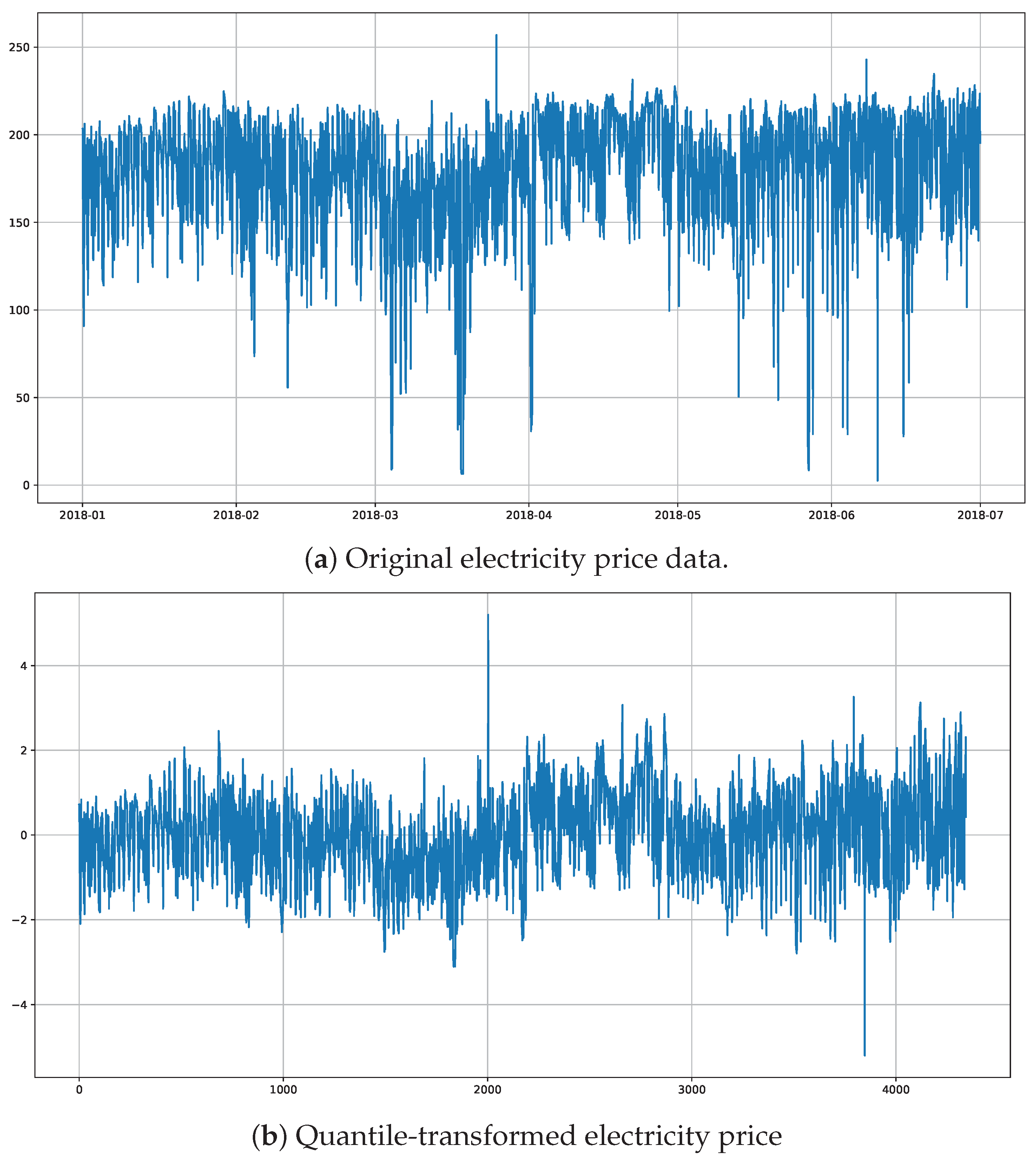
Figure 2 illustrates the evaluation of IDM-WAP electricity prices in panel (a) and the prices after preprocessing in panel (b). Note, in particular, the change in the scale and symmetry of the data after the quantile transformation. The figure illustrates that by applying quantile transformation, the data points are mapped to a normal distribution, spanning the interval [ 4 , 4 ] . This process effectively mitigates the influence of outliers by compressing extreme values towards the center of the distribution, aligning them with the mean of the data.
Table 2 also demonstrates the normalization effect, which summarizes Turkey’s IDM-WAP data and the quantile transformed data statistics. The table presents how quantile transformation reshapes the distribution of IDM-WAP data to standardize them. The transformed data are centered around 0, with a standard deviation of approximately 1, effectively normalizing the dataset and mitigating the influence of outliers by compressing extreme values toward the mean. This process facilitates more reliable statistical analyses and model performance, which assume normality in the data distribution.
In the training of the GANs, we used the quantile-transformed data. The quantile transformation has a mean value ( μ = 0 ), and the symmetric data around the mean have a minimum value of 5.199 and a maximum of 5.199 . Table 2 shows that the quantile transformation pushes the real data into a normal distribution with μ = 0 and σ = 1.004 .

4.2. Implementation Details

We considered RMSprop and Adam optimizer [59] in the numerical experiments. We used the Adam optimizer for SAGAN, LSGAN, DCGAN, DRAGAN, TRANSGAN, BigGAN-DEEP, RALSGAN, and WGAN-GP by considering β 1 = 0 and β 2 = 0.9 as the parameters for DRAGAN and WGAN-GP, β 1 = 0.5 for SAGAN, LSGAN, RALSGAN, and DCGAN, and β 1 = 0 for BigGAN-DEEP and TRANSGAN. We considered the learning rate e 4 for the GANs in the training process. However, unlike others, we set the learning rate to 5 e 5 . We chose c = 0.01 for the weight clipping of WGAN, as it was initially introduced in [46]. In the training of the GANs, the number of epochs utilized was 1.000 , and the batch size considered was 32. The numerical implementations were conducted by using Keras [60].

4.3. Qualitative Analysis

Below, we illustrate the empirical distributions (histograms) and autocorrelation functions (ACF) of all the GANs, along with real data plots. We will considered both qualitative and quantitative judgments for the performance rating of our examined GANs.
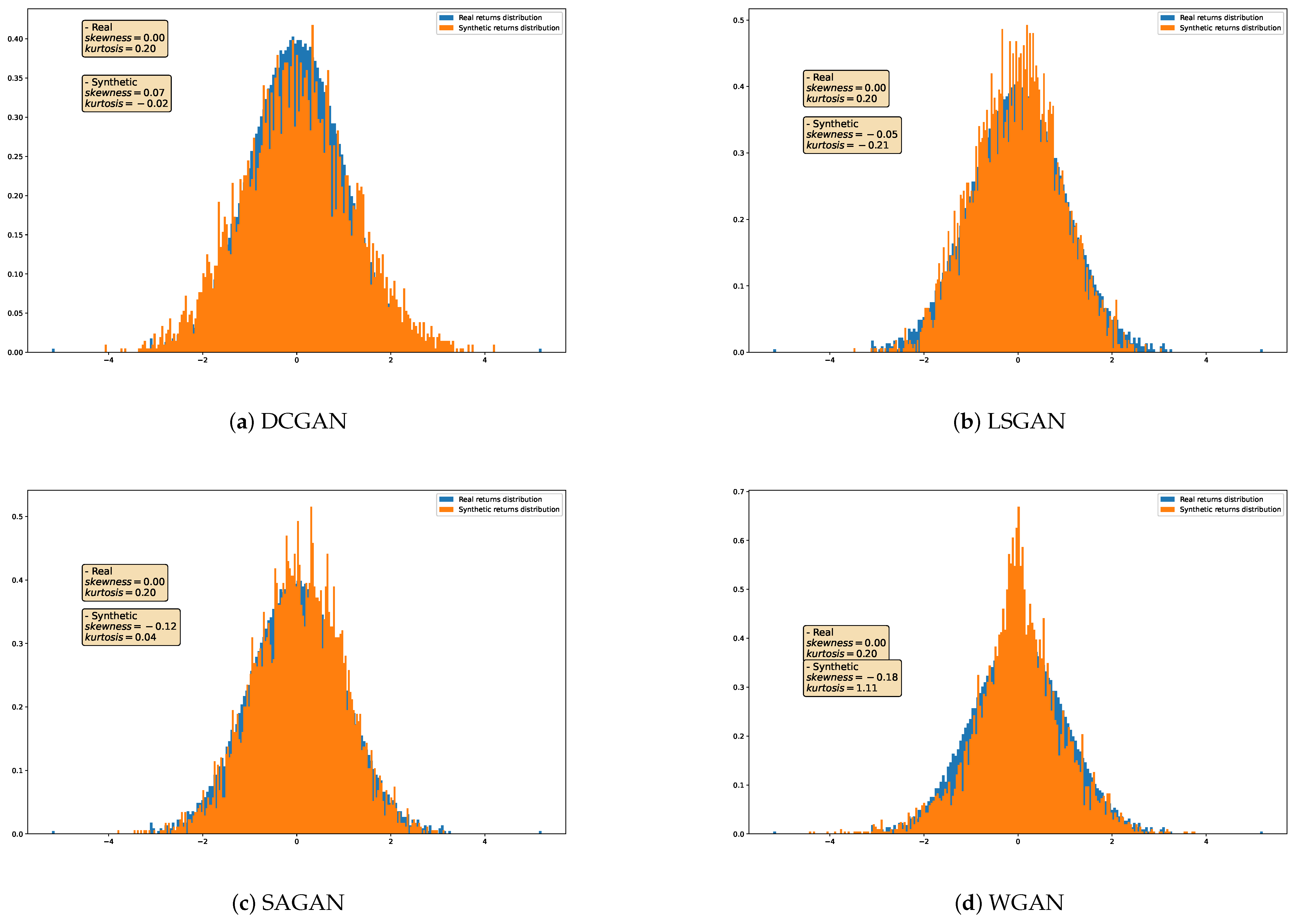
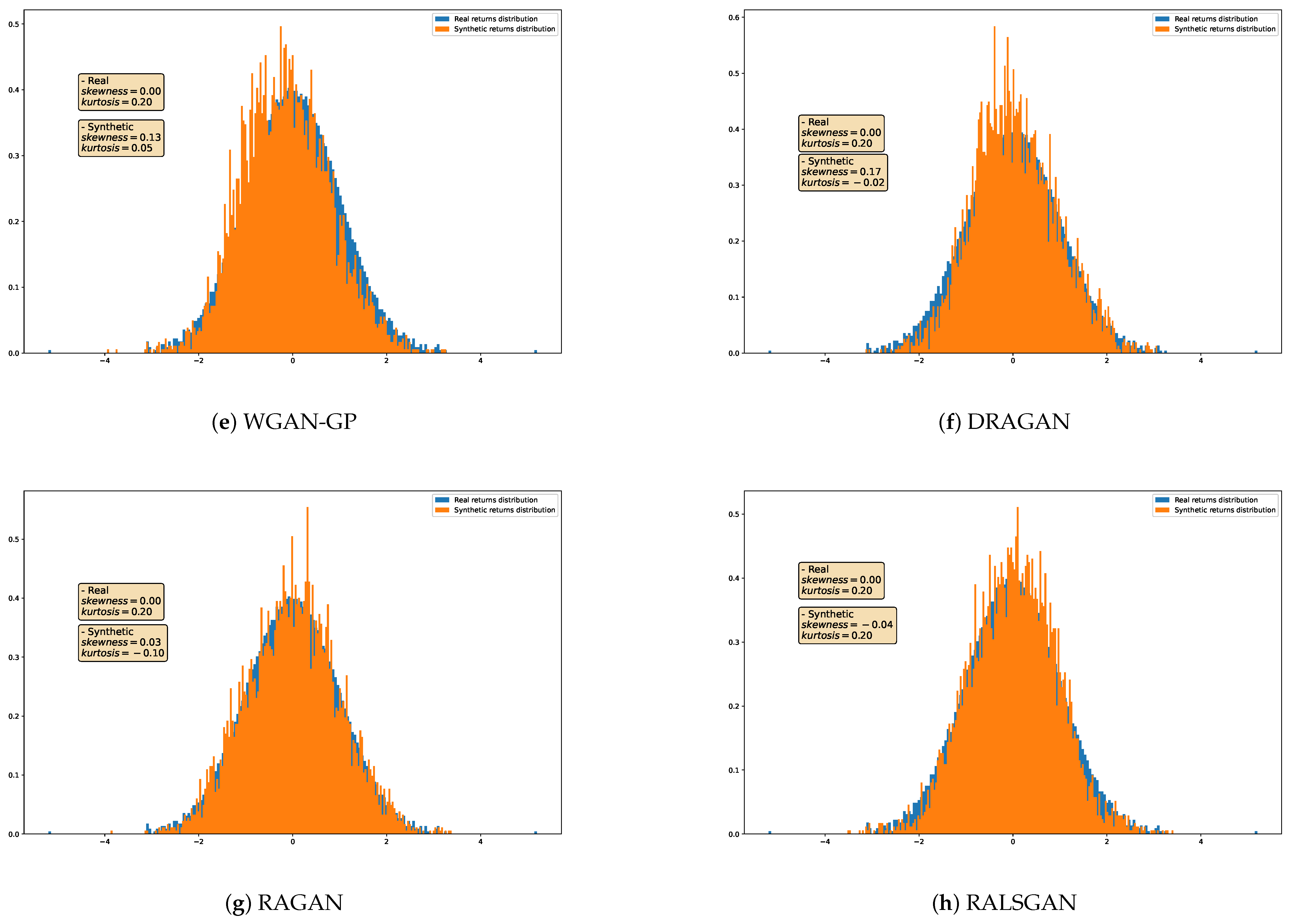
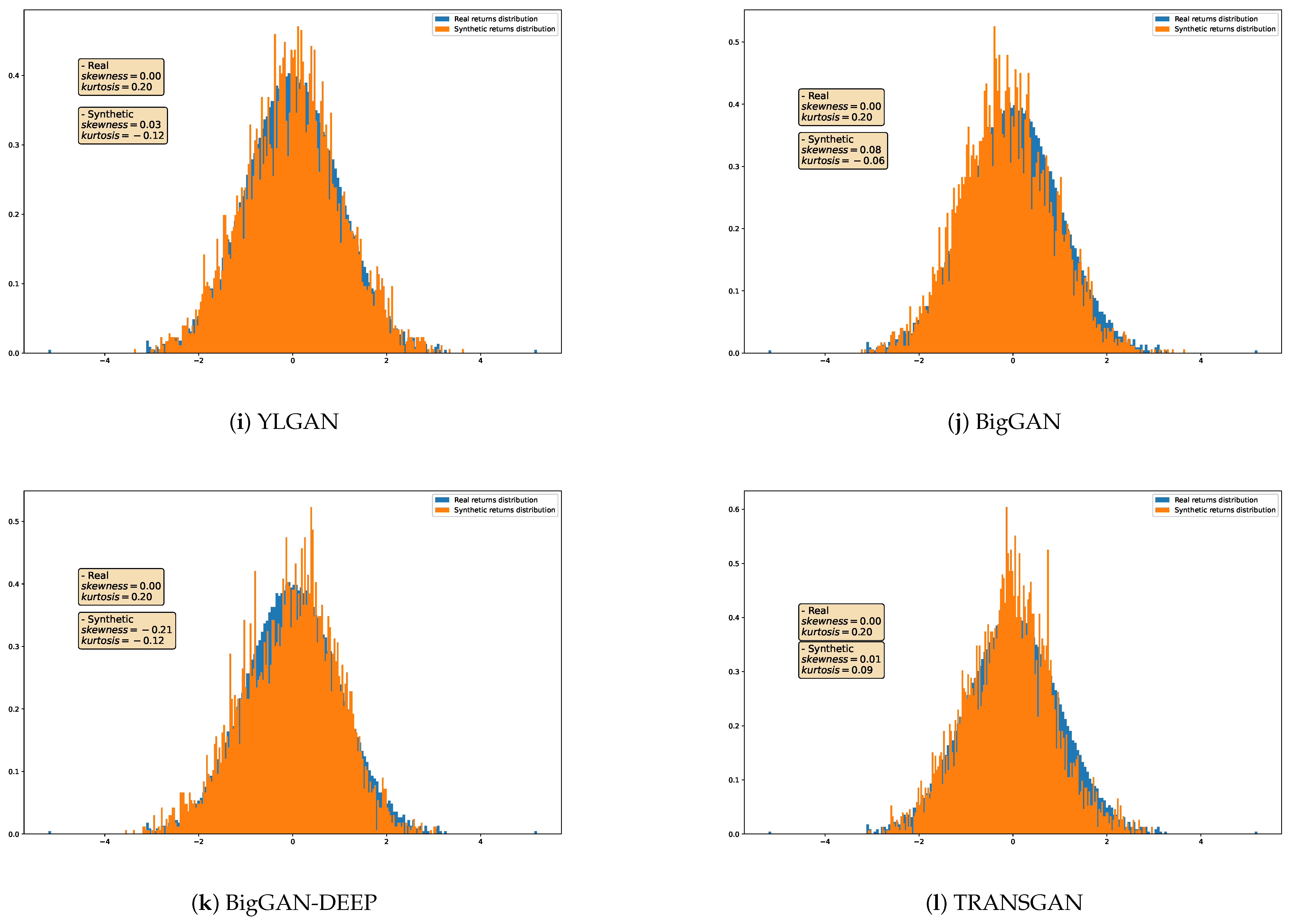
Histograms: Figure 3 compares the probability functions of the original data and the data generated by the corresponding GANs. The figure shows that the GANs perform well overall in replicating the full range of the actual data; however, upon closer examination, the DCGAN, LSGAN, SAGAN, RALSGAN, and BigGAN-DEEP models struggle to capture the left-side outliers, while all the GANs can replicate the right-side outliers. The GANs also produce larger and smaller outliers, with DRAGAN and TRANSGAN demonstrating slightly superior performance in capturing less frequent values across the entire distribution. Among all the GANs evaluated, WGAN-GP exhibits the poorest performance, as the overlap between the real and generated distributions is minimal. Additionally, DCGAN demonstrates a lower peak than the original data. Figure 3 also displays the skewness and kurtosis values of both the real and generated data. DRAGAN exhibits the largest skewness value (0.17), contrasting with the real data skewness (0.00), and BigGAN-DEEP has the lowest skewness value (−0.21). RAGAN and YLGAN demonstrate a skewness closest to the real data (0.03). LSGAN has the lowest kurtosis value (−0.21), and WGAN has the highest kurtosis value (1.11). In contrast, RALSGAN matches the real data kurtosis (0.20). Based on these findings, we conclude that RALSGAN most accurately replicates the data distribution, while WGAN performs the least effectively.
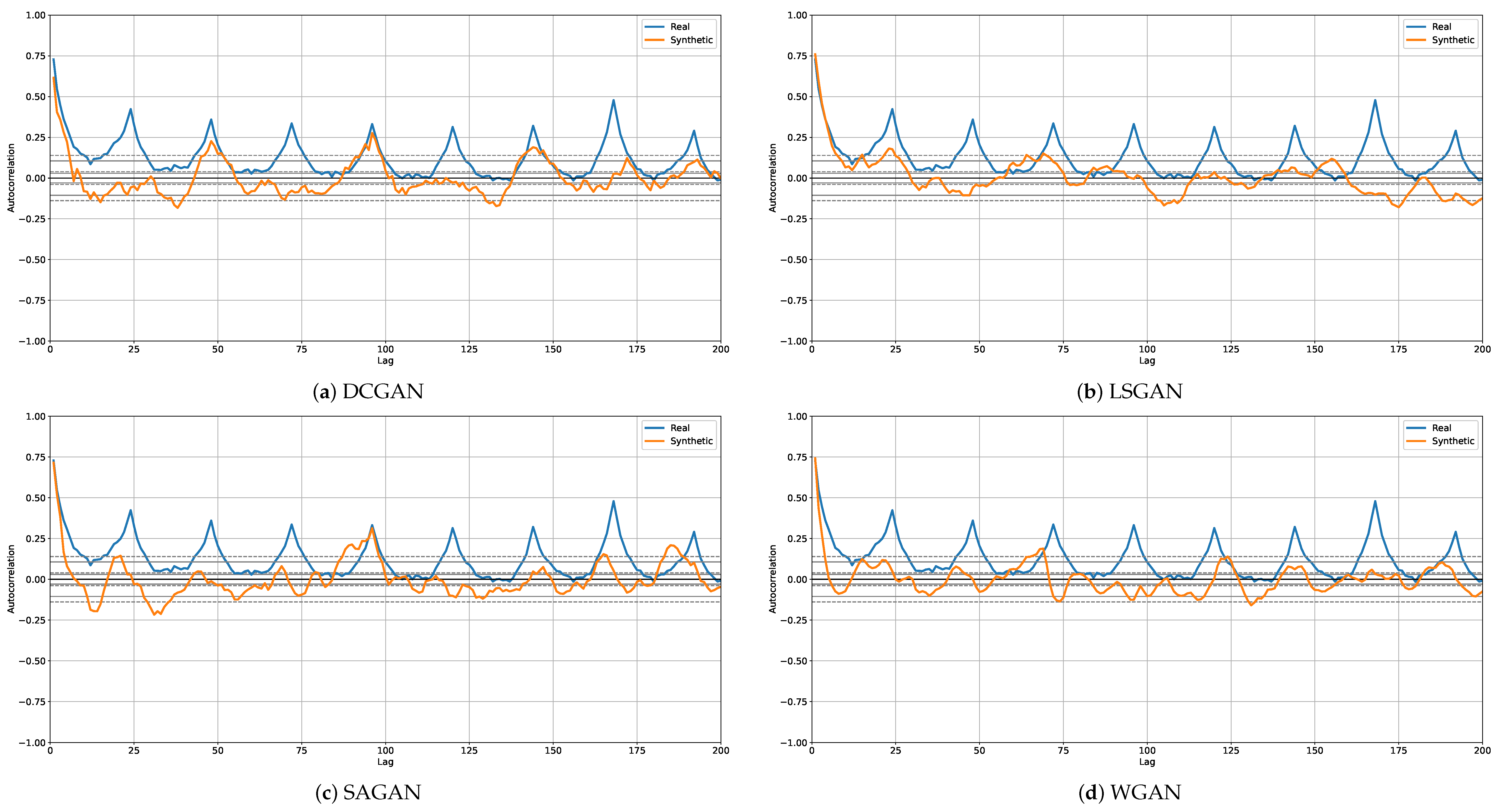
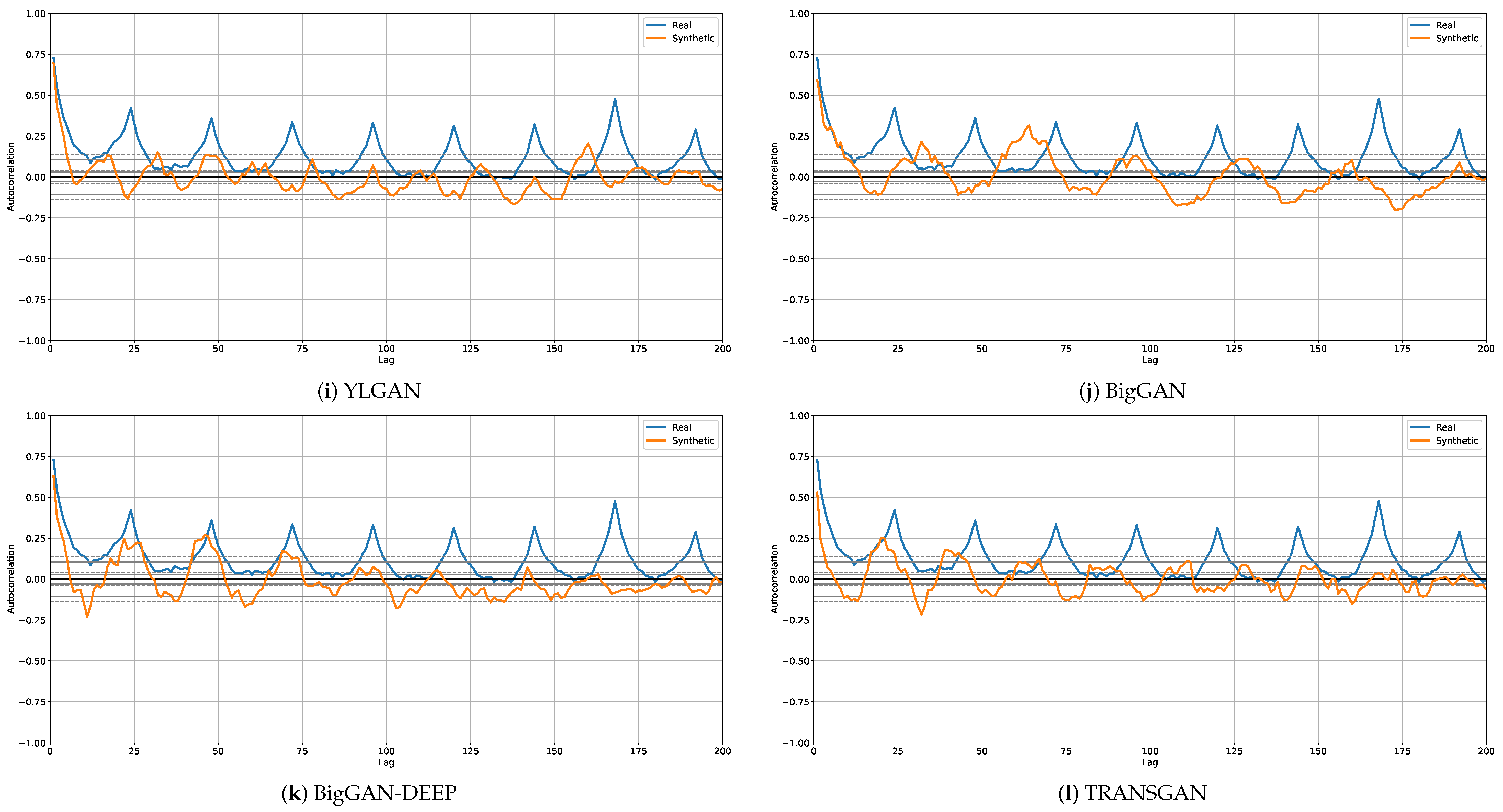
Autocorrelation functions (ACF): Figure 4 presents a comparison of the ACFs of the real data series and the generated data of the various GANs. Most of the GANs perform reasonably well, with DCGAN, SAGAN, DRAGAN, and BigGAN-DEEP showing surprisingly good similarities with the real data. RAGAN and BigGAN do not capture the autocorrelation structure well.
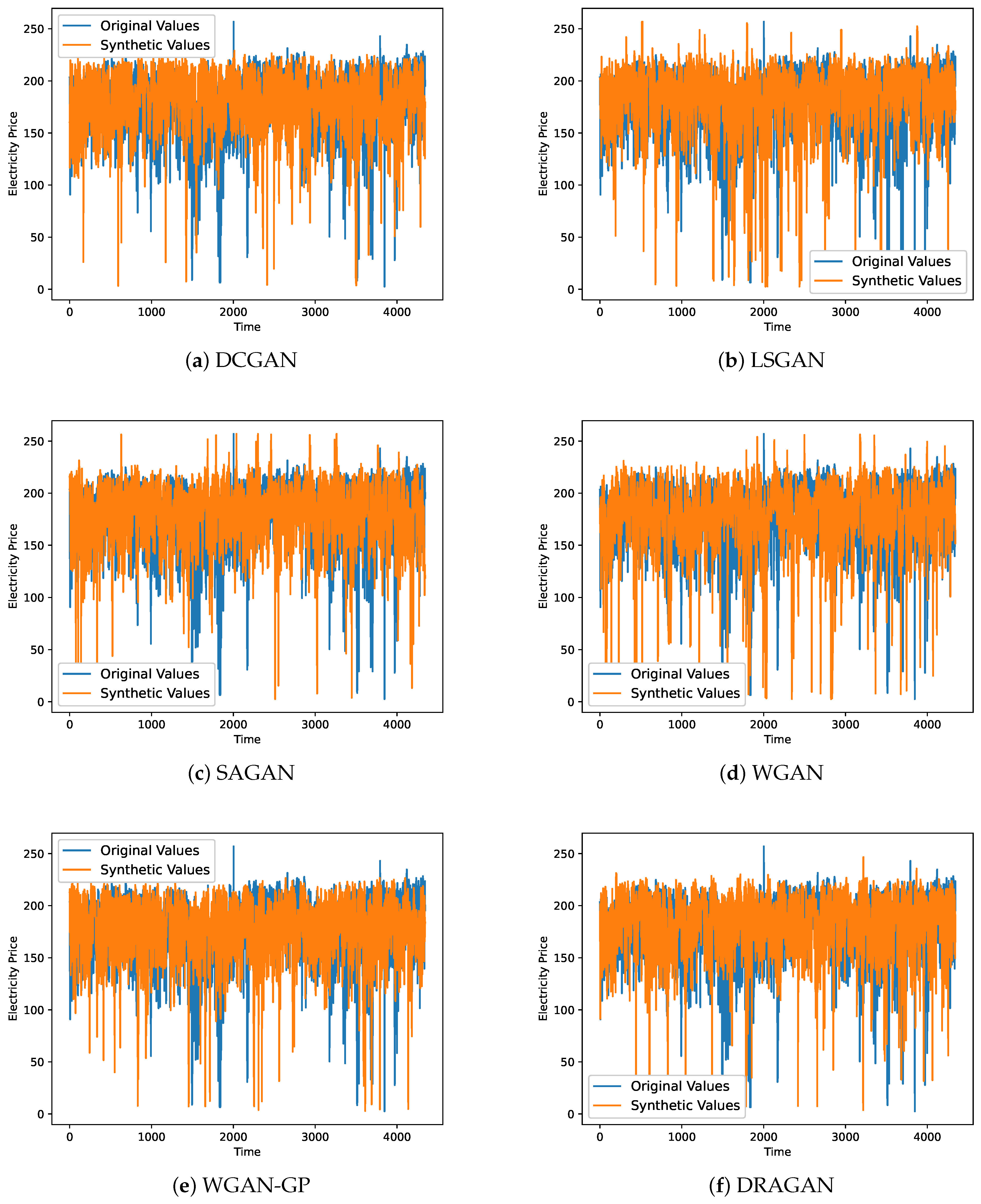
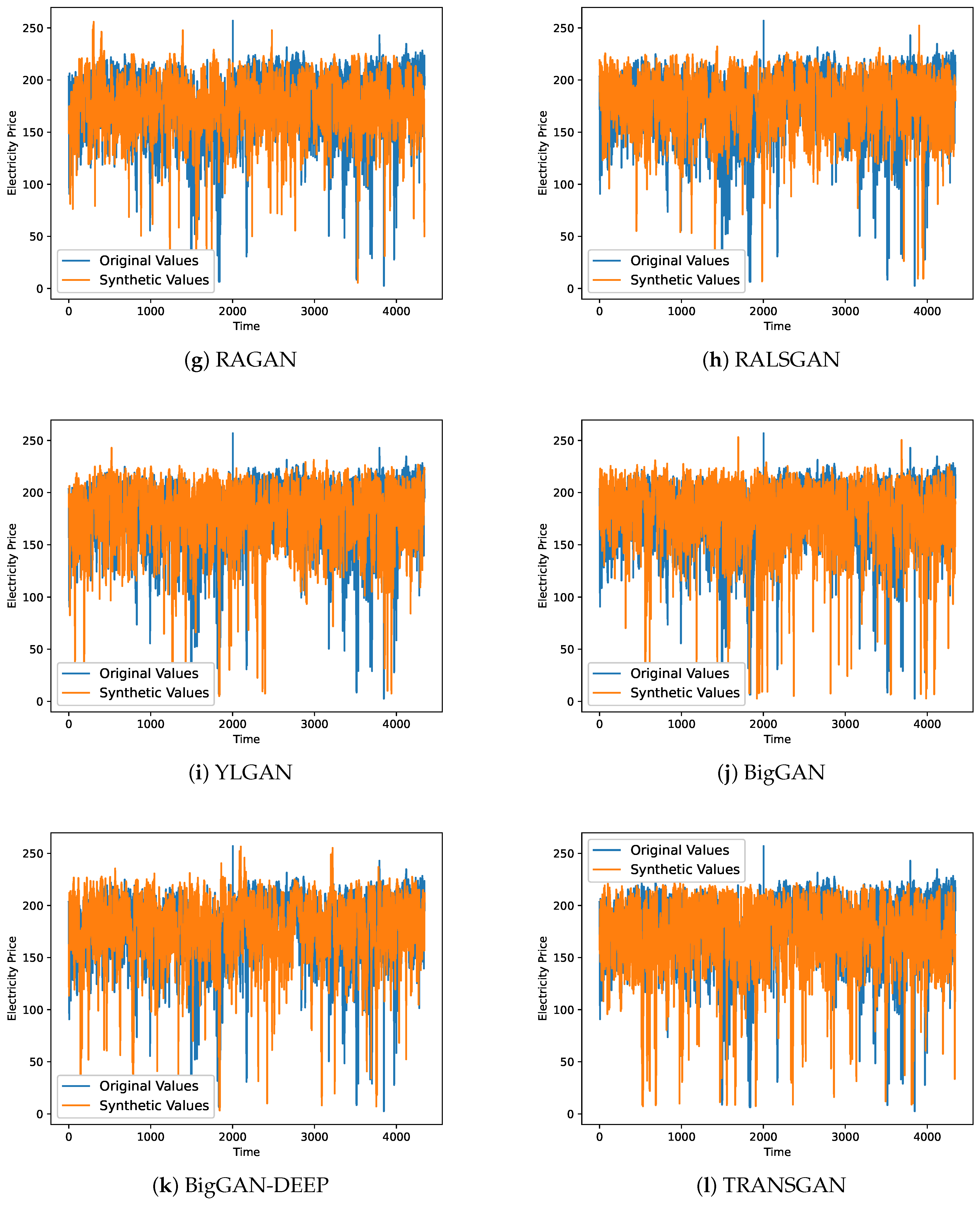
Visualizing the generated and real data series: Figure 5 illustrates a comparison between the original data before preprocessing and the generated data. The figure reveals that the GANs are good at capturing the outliers at the bottom of the data while generally suffering the outliers at the top of the data. LSGAN, SAGAN, WGAN, RAGAN, BigGAN, and BigGAN-DEEP generate synthetic electricity prices at the top of the data. However, most of the GANs generated more outliers at the top of the data. Only BigGAN and BigGAN-DEEP generated two outliers at the top.
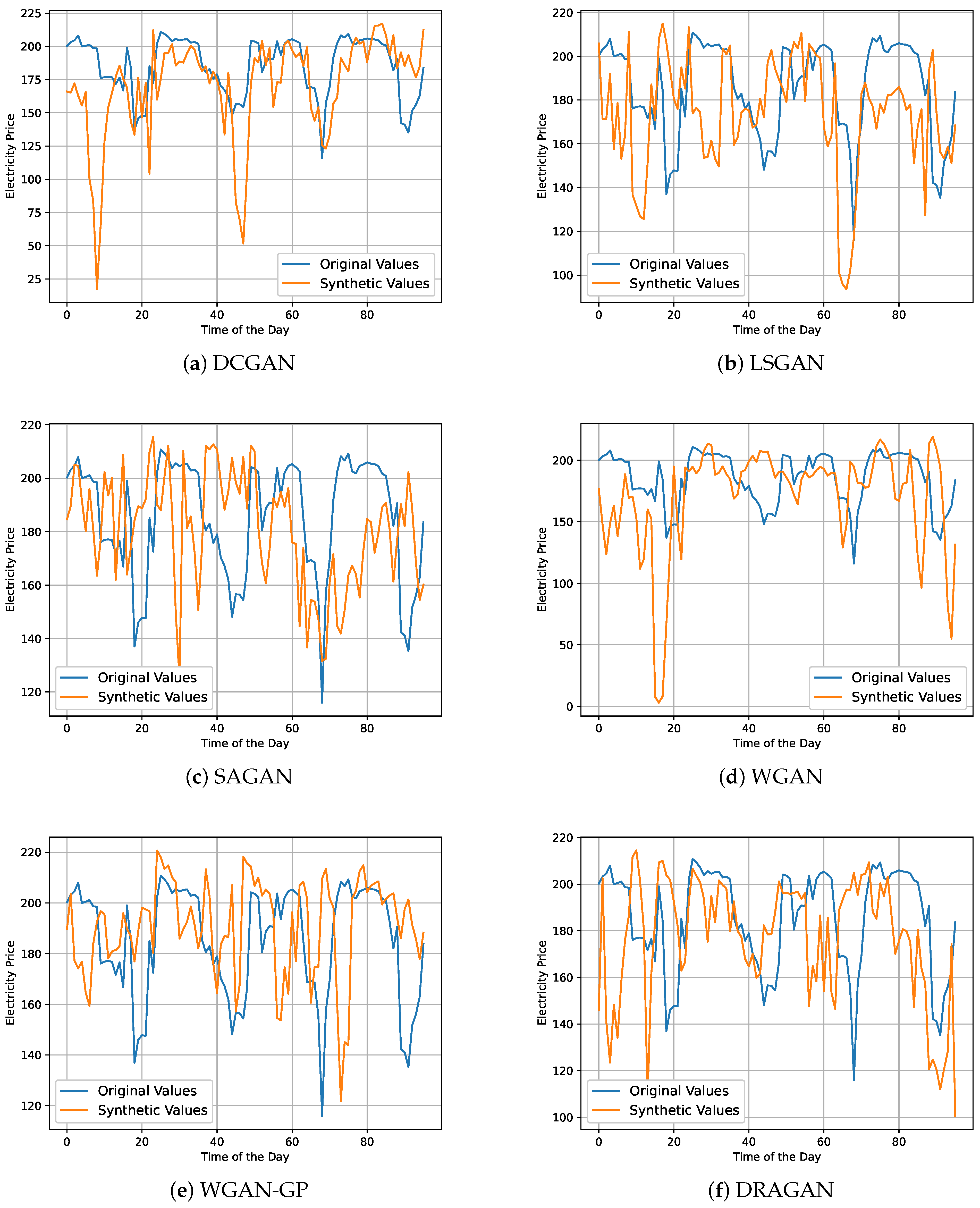
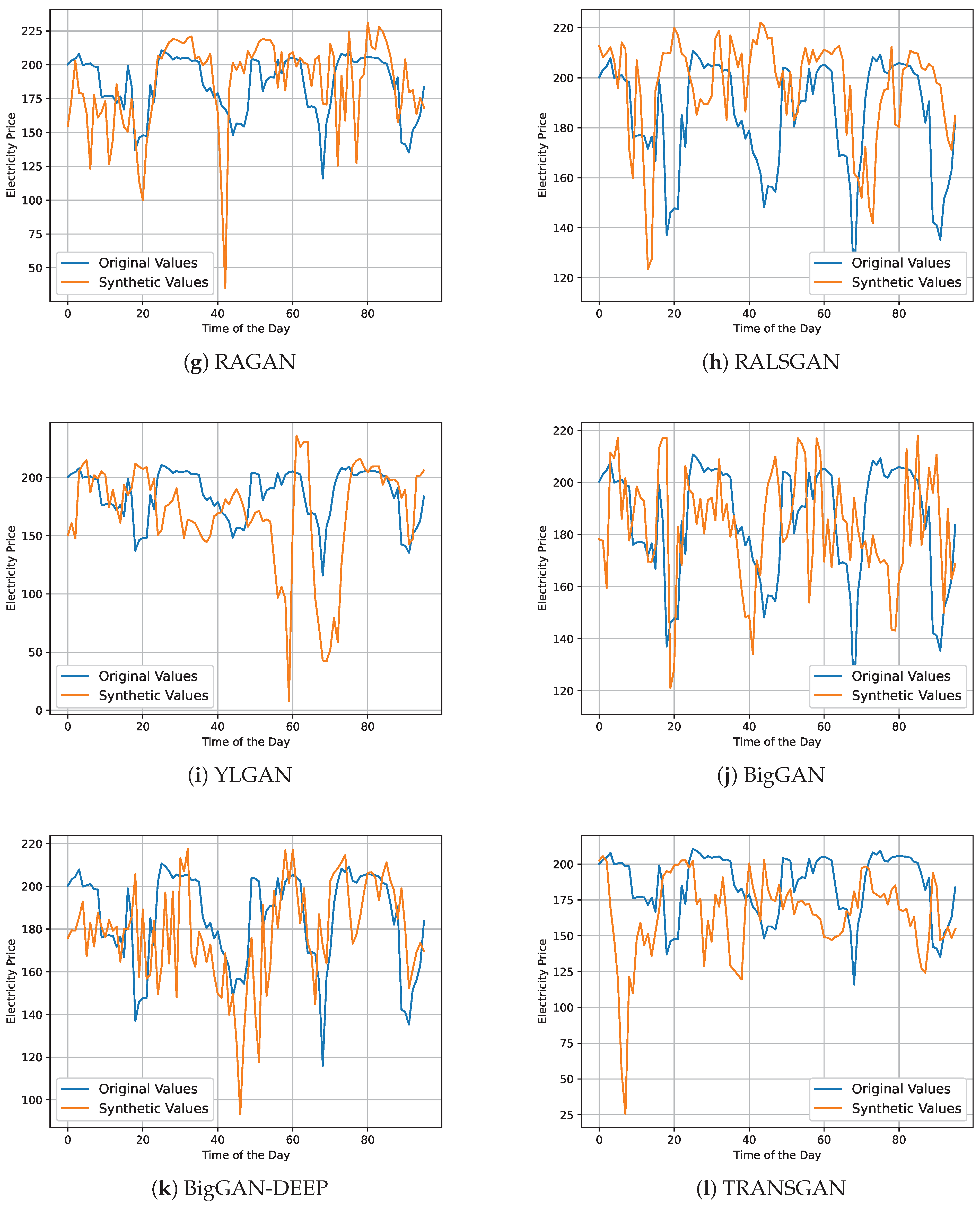
In Figure 6, we present a random selection of 96 h. The figure reveals some of the following trends. Figure 6 illustrates the similarity between the generated datasets and the behavior of electricity prices. It seems that DCGAN and BigGAN-Deep mimic quite a good hourly pattern (lower prices at night and higher prices in the daytime) in the data. For the other GANs, we also observe a shift in this pattern; e.g., for SAGAN, between hours 60 and 100, the peak is much later than in the real data. Another interesting observation is that for some of the GANs, we see a higher frequency of oscillations than in the real data, e.g., for SAGAN, BigGAN, and BigGAN-DEEP. However, based on just one simulated path, it is impossible to decide which GAN is superior to all others. On the positive side, differentiating between the real and generated data appears to be challenging.
Statistical analysis: Table 3 includes two evaluation metrics and the descriptive statistics of the synthetic data generated by the GANs. One metric is the KS statistic of the two-sided Kolmogorov–Smirnov (KS) test, with the null hypothesis that both the quantile-transformed original data and the synthetic samples produced by the GANs come from the same underlying distribution. Note that we focus here on the direct output of the GANs without using the back transformation stemming from the quantile transformation. It is defined as the maximum disparity between the distribution functions of two empirical distributions (see [61]). A low KS statistic suggests that the null hypothesis—asserting the real and synthetic data follow the same distribution—cannot be rejected. The height of the p-values indicates how strongly we can believe in the equality of the two empirical distributions. As all of the p-values are far from the usual choices of the significance level, the null hypothesis is never rejected. However, the p-values of DCGAN and TRANSGAN are lower than those of the other ones. This is already an indicator of the excellent performance of the tested GANs.
Furthermore, we used the ACE test introduced by Yilmaz [12] as the second evaluation metric to decide which of the investigated models is the superior GAN. The ACE test is based on the prediction interval coverage probability (PICP) as a metric, quantifying the proportion of real data points falling within the prediction intervals (PIs) determined by the generated data’s quantiles. PICP equals the nominal confidence of the PIs and covers the percentage of the real data points. The ACE test corresponds to the difference between PICP and the nominal confidence level ( α ) , providing insight into the accuracy of the GAN-generated PIs.
Table 3 presents the statistical properties of the generated data after back transformation. As the table shows, the mean and standard deviation of the generated data from all GANs are relatively close to the original data mean (178.130) and standard deviation (33.096) given in Table 2. BigGAN-DEEP has the closest mean (178.04) to the original data mean, whereas LSGAN has the most distant mean (184.09). Conversely, WGAN exhibits a standard deviation of 32.99 , which is closest to that of the original data ( 33.096 ), whereas a standard deviation of 28.22 for DRAGAN shows the largest deviation. Surprisingly, BigGAN-DEEP has an identical max value (256.93) to the original data max value (256.93), and WGAN-GP has a distant max value (225.32). WGAN has the closest min value (2.55), and the DCGAN has the most distant min value (16.99). The last column in Table 3 presents the total computation cost (in minutes) of the GANs we implemented in the study. We observe significant variations across different models. The DCGAN, LSGAN, WGAN, WGAN-GP, DRAGAN, RAGAN, RALSGAN, and YLGAN models generally have lower computational costs, ranging from approximately 23.64 to 52.03 min. TRANSGAN exhibits the highest computational cost among all the models, with a value of roughly 159.99 min. DCGAN, LSGAN, and others with lower computational costs have simpler architectures or require fewer computational resources during training and generation. BigGAN, BigGAN-DEEP, and TRANSGAN likely have higher computational costs due to more complex architectures, larger model sizes, or more intensive operations, such as self-attention mechanisms (in the case of TRANSGAN). TRANSGAN particularly stands out in terms of the highest computational cost, which is attributed to its transformer-based architecture and the computational demands of processing structured data with self-attention mechanisms. It is apparent that as the GAN architecture becomes more complicated, the computational cost increases drastically, while the efficiency (indicated by ACE), moments, and KS do not increase.
Based on the visualizations and statistical analysis, it is clear that all GANs generate realistic synthetic electricity price data. However, the visualizations and classical statistics are insufficient for identifying the best GANs. On the other hand, the ACE values at least provide a hint about the closest generated data to the real data. Hence, we may conclude the best GANs by considering the ACE values. Consequently, by considering the ACE values in Table 3, we may conclude that DRAGAN is the best GAN among the alternatives. Although WGAN has only a good ACF performance, its excellent ACE, low computation time, and low complexity, paired with good moment-matching, make it a serious candidate to consider, too. More importantly, GANs that have modified objective functions and specialized neural network structures fail to dominate the less cumbersome GANs, and they are computationally more expensive.

5. Conclusions

This study has established the efficacy of GANs in generating synthetic electricity price data, providing valuable insights and practical applications for participants in the energy market. We have demonstrated the capability of the models to mimic the complex dynamics and statistical properties of electricity price data through a detailed empirical analysis of various GAN architectures. The key contributions of our research are summarized as follows:
  • Replication of complex dynamics: We conducted a comprehensive empirical analysis using diverse GAN architectures and demonstrated the ability of GANs to replicate the complex dynamics and statistical characteristics of electricity price data.
  • Comprehensive performance evaluation: We leveraged a robust evaluation methodology comprising qualitative and quantitative techniques such as histograms, visual comparisons, ACF, KS statistics, and the ACE test. Further, we thoroughly assessed the performance and computational costs associated with various GAN architectures and provided valuable guidance to practitioners on utilizing synthetic data for strategy testing, risk model validation, and decision-making enhancement in the energy market, assessing the strengths and limitations of each GAN and offering practical guidance for their application in strategy testing, risk model validation, and decision-making in the energy market.
  • Quality and utility of synthetic data: We generated high-quality synthetic electricity price data that can help address privacy concerns and data scarcity issues and enable market participants to overcome the limitations related to restricted access to real-world data, facilitating innovation and informed decision-making.
  • Insights into computational efficiency: We highlighted significant variations in computational costs across the various GAN architectures; we showed that simpler GANs often offer a favorable balance between performance and computational efficiency compared to more complex models.
  • Addressing privacy and data scarcity: We highlighted the potential of high-quality synthetic electricity price data to address privacy concerns and data scarcity issues, enabling market participants to overcome the limitations associated with restricted access to real-world data.
The study can be extended by considering the following future research directions.
  • Exploring novel GAN architectures, optimization techniques, and evaluation metrics to enhance the precision and robustness of synthetic data generation might increase the value of GANs;
  • Investigating the applicability of synthetic data in other domains within the energy sector to broaden impact and stimulate interdisciplinary collaborations may increase modeling efficiency and decrease investment risk in energy markets.
In conclusion, this research provides a comprehensive evaluation of GANs for synthetic electricity price data generation, offering valuable tools and insights for energy market participants and setting the stage for future advancements in this field.

Author Contributions

B.Y.: Conceptualization, Methodology, Investigation, Validation, Visualization, Writing an original draft, Reviewing and editing. R.K.: Supervision, Writing the final draft, Methodology, Reviewing, and Editing. S.D.: Conceptualization, Supervision, Reviewing, and Editing. C.L.: Conceptualization, Methodology, Investigation, Reviewing, and Editing. All authors have read and agreed to the published version of the manuscript.

Funding

This research received no external funding.

Institutional Review Board Statement

Not applicable.

Informed Consent Statement

Not applicable.

Data Availability Statement

The data used in this work are publicly open to all interested researchers via  https://seffaflik.epias.com.tr/home, accessed on 13 May 2024.

Conflicts of Interest

The authors declare no conflicts of interest.

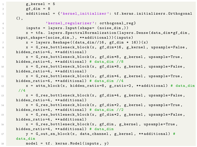
Appendix A. A Sample Code for GANs Training (BigGAN-DEEP)

Listing A1. The Generator.
Commodities 03 00016 i001
Listing A2. The Discriminator.
Commodities 03 00016 i002
Listing A3. The Discriminator Loss.
Commodities 03 00016 i003
Listing A4. The Generator Loss.
Commodities 03 00016 i004
Listing A5. Optimizers.
Commodities 03 00016 i005
Listing A6. Training.
Commodities 03 00016 i006

References

  1. Zhang, J.; Tan, Z.; Wei, Y. An adaptive hybrid model for short term electricity price forecasting. Appl. Energy 2020, 258, 114087. [Google Scholar] [CrossRef]
  2. Yang, Z.; Ce, L.; Lian, L. Electricity price forecasting by a hybrid model, combining wavelet transform, ARMA and kernel-based extreme learning machine methods. Appl. Energy 2017, 190, 291–305. [Google Scholar] [CrossRef]
  3. Gulrajani, I.; Ahmed, F.; Arjovsky, M.; Dumoulin, V.; Courville, A. Improved Training of Wasserstein GANs. arXiv 2017, arXiv:1704.00028. [Google Scholar]
  4. Zhu, J.Y.; Park, T.; Isola, P.; Efros, A.A. Unpaired Image-to-Image Translation using Cycle-Consistent Adversarial Networks. arXiv 2020, arXiv:1703.10593. [Google Scholar]
  5. Chen, Y.; Lai, Y.K.; Liu, Y.J. Cartoongan: Generative adversarial networks for photo cartoonization. In Proceedings of the IEEE Conference on Computer Vision and Pattern Recognition, Salt Lake City, UT, USA, 18–23 June 2018; pp. 9465–9474. [Google Scholar]
  6. Jin, Y.; Zhang, J.; Li, M.; Tian, Y.; Zhu, H.; Fang, Z. Towards the automatic anime characters creation with generative adversarial networks. arXiv 2017, arXiv:1708.05509. [Google Scholar]
  7. Efimov, D.; Xu, D.; Kong, L.; Nefedov, A.; Anandakrishnan, A. Using generative adversarial networks to synthesize artificial financial datasets. arXiv 2020, arXiv:2002.02271. [Google Scholar]
  8. Yu, L.; Zhang, W.; Wang, J.; Yu, Y. SeqGAN: Sequence Generative Adversarial Nets with Policy Gradient. arXiv 2017, arXiv:1609.05473. [Google Scholar]
  9. Li, J.; Chen, Z.; Cheng, L.; Liu, X. Energy data generation with Wasserstein deep convolutional generative adversarial networks. Energy 2022, 257, 124694. [Google Scholar] [CrossRef]
  10. Wang, Z.; Hong, T. Generating realistic building electrical load profiles through the Generative Adversarial Network (GAN). Energy Build. 2020, 224, 110299. [Google Scholar] [CrossRef]
  11. Yilmaz, B.; Korn, R. Synthetic demand data generation for individual electricity consumers: Generative Adversarial Networks (GANs). Energy AI 2022, 9, 100161. [Google Scholar] [CrossRef]
  12. Yilmaz, B. A scenario framework for electricity grid using Generative Adversarial Networks. Sustain. Energy Grids Netw. 2023, 36, 101157. [Google Scholar] [CrossRef]
  13. Yilmaz, B. Generative adversarial network for load data generation: Türkiye energy market case. Math. Model. Numer. Simul. Appl. 2023, 3, 141–158. [Google Scholar] [CrossRef]
  14. Wiese, M.; Knobloch, R.; Korn, R.; Kretschmer, P. Quant GANs: Deep generation of financial time series. Quant. Financ. 2020, 20, 1419–1440. [Google Scholar] [CrossRef]
  15. Li, J.; Wang, X.; Lin, Y.; Sinha, A.; Wellman, M.P. Generating Realistic Stock Market Order Streams. arXiv 2020, arXiv:2006.04212. [Google Scholar] [CrossRef]
  16. Dwibedi, D.; Misra, I.; Hebert, M. Cut, paste and learn: Surprisingly easy synthesis for instance detection. In Proceedings of the IEEE International Conference on Computer Vision, Venice, Italy, 22–29 October 2017; pp. 1301–1310. [Google Scholar] [CrossRef]
  17. Georgakis, G.; Mousavian, A.; Berg, A.C.; Kosecka, J. Synthesizing training data for object detection in indoor scenes. arXiv 2017, arXiv:1702.07836. [Google Scholar]
  18. Goodfellow, I.J.; Pouget-Abadie, J.; Mirza, M.; Xu, B.; Warde-Farley, D.; Ozair, S.; Courville, A.; Bengio, Y. Generative Adversarial Networks. arXiv 2014, arXiv:1406.2661. [Google Scholar]
  19. de Souza, V.L.T.; Marques, B.A.D.; Batagelo, H.C.; Gois, J.P. A review on generative adversarial networks for image generation. Comput. Graph. 2023, 114, 13–25. [Google Scholar] [CrossRef]
  20. Wang, T. Research and Application Analysis of Correlative Optimization Algorithms for GAN. Highlights Sci. Eng. Technol. 2023, 57, 141–147. [Google Scholar] [CrossRef]
  21. Gui, J.; Sun, Z.; Wen, Y.; Tao, D.; Ye, J. A review on generative adversarial networks: Algorithms, theory, and applications. IEEE Trans. Knowl. Data Eng. 2021, 35, 3313–3332. [Google Scholar] [CrossRef]
  22. Tavse, S.; Varadarajan, V.; Bachute, M.; Gite, S.; Kotecha, K. A systematic literature review on applications of GAN-synthesized images for brain MRI. Future Internet 2022, 14, 351. [Google Scholar] [CrossRef]
  23. Yilmaz, B.; Korn, R. A Comprehensive guide to Generative Adversarial Networks (GANs) and application to individual electricity demand. Expert Syst. Appl. 2024, 250, 123851. [Google Scholar] [CrossRef]
  24. Uddin, K.; Jeong, T.H.; Oh, B.T. Counter-act against GAN-based attacks: A collaborative learning approach for anti-forensic detection. Appl. Soft Comput. 2024, 153, 111287. [Google Scholar] [CrossRef]
  25. Wiese, M.; Bai, L.; Wood, B.; Buehler, H. Deep Hedging: Learning to Simulate Equity Option Markets. arXiv 2019, arXiv:1911.01700. [Google Scholar]
  26. Yilmaz, B. Housing GANs: Deep Generation of Housing Market Data. Comput. Econ. 2023, 1–16. [Google Scholar] [CrossRef]
  27. van Rhijn, J.; Oosterlee, C.W.; Grzelak, L.A.; Liu, S. Monte carlo simulation of sdes using gans. Jpn. J. Ind. Appl. Math. 2023, 40, 1359–1390. [Google Scholar] [CrossRef]
  28. Wang, Z.; She, Q.; Ward, T.E. Generative adversarial networks in computer vision: A survey and taxonomy. ACM Comput. Surv. (CSUR) 2021, 54, 1–38. [Google Scholar] [CrossRef]
  29. Borji, A. Pros and cons of GAN evaluation measures: New developments. Comput. Vis. Image Underst. 2022, 215, 103329. [Google Scholar] [CrossRef]
  30. Borji, A. Pros and cons of gan evaluation measures. Comput. Vis. Image Underst. 2019, 179, 41–65. [Google Scholar] [CrossRef]
  31. Sutherland, D.J.; Tung, H.Y.; Strathmann, H.; De, S.; Ramdas, A.; Smola, A.; Gretton, A. Generative models and model criticism via optimized maximum mean discrepancy. arXiv 2016, arXiv:1611.04488. [Google Scholar]
  32. Salimans, T.; Goodfellow, I.; Zaremba, W.; Cheung, V.; Radford, A.; Chen, X. Improved techniques for training GANs. Adv. Neural Inf. Process. Syst. 2016, 29, 2234–2242. [Google Scholar]
  33. Heusel, M.; Ramsauer, H.; Unterthiner, T.; Nessler, B.; Hochreiter, S. Gans trained by a two time-scale update rule converge to a local nash equilibrium. Adv. Neural Inf. Process. Syst. 2017, 30, 6629–6640. [Google Scholar]
  34. Van der Maaten, L.; Hinton, G. Visualizing data using t-SNE. J. Mach. Learn. Res. 2008, 9, 2579–2605. [Google Scholar]
  35. Bryant, F.B.; Yarnold, P.R. Principal-components analysis and exploratory and confirmatory factor analysis. In Reading and Understanding Multivariate Statistics; American Psychological Association: Washington, DC, USA, 1995; pp. 99–136. [Google Scholar]
  36. Yoon, J.; Jarrett, D.; van der Schaar, M. Time-series Generative Adversarial Networks. In Advances in Neural Information Processing Systems; Wallach, H., Larochelle, H., Beygelzimer, A., d’Alché-Buc, F., Fox, E., Garnett, R., Eds.; Curran Associates, Inc.: Red Hook, NY, USA, 2019; Volume 32. [Google Scholar]
  37. Esteban, C.; Hyland, S.L.; Rätsch, G. Real-valued (Medical) Time Series Generation with Recurrent Conditional GANs. arXiv 2017, arXiv:1706.02633. [Google Scholar]
  38. Mogren, O. C-RNN-GAN: Continuous recurrent neural networks with adversarial training. arXiv 2016, arXiv:1611.09904. [Google Scholar]
  39. Hanif, M.; Shahzad, M.K.; Mehmood, V.; Saleem, I. EPFG: Electricity price forecasting with enhanced Gans neural network. IETE J. Res. 2023, 69, 6473–6482. [Google Scholar] [CrossRef]
  40. Yuan, R.; Wang, B.; Mao, Z.; Watada, J. Multi-objective wind power scenario forecasting based on PG-GAN. Energy 2021, 226, 120379. [Google Scholar] [CrossRef]
  41. Demir, S.; Mincev, K.; Kok, K.; Paterakis, N.G. Data augmentation for time series regression: Applying transformations, autoencoders and adversarial networks to electricity price forecasting. Appl. Energy 2021, 304, 117695. [Google Scholar] [CrossRef]
  42. Cheng, T.; Li, X.; Li, Y. Hybrid deep learning techniques for providing incentive price in electricity market. Comput. Electr. Eng. 2022, 99, 107808. [Google Scholar] [CrossRef]
  43. Wang, X.; Li, F.; Zhao, J.; Olama, M.; Dong, J.; Shuai, H.; Kuruganti, T. Tri-level hybrid interval-stochastic optimal scheduling for flexible residential loads under GAN-assisted multiple uncertainties. Int. J. Electr. Power Energy Syst. 2023, 146, 108672. [Google Scholar] [CrossRef]
  44. Dimitriadis, C.N.; Tsimopoulos, E.G.; Georgiadis, M.C. A Review on the Complementarity Modelling in Competitive Electricity Markets. Energies 2021, 14, 7133. [Google Scholar] [CrossRef]
  45. Villani, C. Optimal Transport: Old and New; Springer: Berlin/Heidelberg, Germany, 2009; Volume 338. [Google Scholar] [CrossRef]
  46. Arjovsky, M.; Chintala, S.; Bottou, L. Wasserstein generative adversarial networks. arXiv 2017, arXiv:1701.07875. [Google Scholar]
  47. Mao, X.; Li, Q.; Xie, H.; Lau, R.Y.K.; Wang, Z.; Smolley, S.P. Least Squares Generative Adversarial Networks. arXiv 2017, arXiv:1611.04076. [Google Scholar]
  48. Zhang, H.; Goodfellow, I.; Metaxas, D.; Odena, A. Self-Attention Generative Adversarial Networks. arXiv 2018, arXiv:1805.08318. [Google Scholar]
  49. Jolicoeur-Martineau, A. The relativistic discriminator: A key element missing from standard GAN. arXiv 2018, arXiv:1807.00734. [Google Scholar]
  50. Radford, A.; Metz, L.; Chintala, S. Unsupervised representation learning with deep convolutional generative adversarial networks. arXiv 2015, arXiv:1511.06434. [Google Scholar]
  51. Kodali, N.; Abernethy, J.; Hays, J.; Kira, Z. On convergence and stability of gans. arXiv 2017, arXiv:1705.07215. [Google Scholar]
  52. Brock, A.; Donahue, J.; Simonyan, K. Large Scale GAN Training for High Fidelity Natural Image Synthesis. arXiv 2018, arXiv:1809.11096. [Google Scholar]
  53. Daras, G.; Odena, A.; Zhang, H.; Dimakis, A.G. Your Local GAN: Designing Two Dimensional Local Attention Mechanisms for Generative Models. In Proceedings of the IEEE/CVF Conference on Computer Vision and Pattern Recognition (CVPR), Seattle, WA, USA, 13–19 June 2020. [Google Scholar]
  54. Zhang, Z.; Wu, M. Predicting real-time locational marginal prices: A gan-based approach. IEEE Trans. Power Syst. 2021, 37, 1286–1296. [Google Scholar] [CrossRef]
  55. Avkhimenia, V.; Weis, T.; Musilek, P. Generation of synthetic ampacity and electricity pool prices using generative adversarial networks. In Proceedings of the 2021 IEEE Electrical Power and Energy Conference (EPEC), Virtual, 22–31 October 2021; pp. 225–230. [Google Scholar]
  56. Dogariu, M.; Ştefan, L.D.; Boteanu, B.A.; Lamba, C.; Kim, B.; Ionescu, B. Generation of realistic synthetic financial time-series. Acm Trans. Multimed. Comput. Commun. Appl. (TOMM) 2022, 18, 1–27. [Google Scholar] [CrossRef]
  57. Meyer-Brandis, T.; Tankov, P. Multi-factor jump-diffusion models of electricity prices. Int. J. Theor. Appl. Financ. 2008, 11, 503–528. [Google Scholar] [CrossRef]
  58. Wunderlich, A.; Sklar, J. Data-driven modeling of noise time series with convolutional generative adversarial networks. Mach. Learn. Sci. Technol. 2023, 4, 035023. [Google Scholar] [CrossRef]
  59. Kingma, D.P.; Ba, J. Adam: A Method for Stochastic Optimization. arXiv 2017, arXiv:1412.6980. [Google Scholar]
  60. Chollet, F. Keras. GitHub. 2015. Available online: https://github.com/fchollet/keras (accessed on 13 May 2024).
  61. Hodges, J.L. The significance probability of the Smirnov two-sample test. Arkiv Mat. 1958, 3, 469–486. [Google Scholar] [CrossRef]
Figure 1. An illustration of the general architecture of a GAN (taken from [13]).
Commodities 03 00016 g001
Figure 2. Time series of Turkey’s IDM-WAP electricity price and its quantile-transformed version.
Commodities 03 00016 g002
Figure 3. Distributional properties of synthetic and original data.
Commodities 03 00016 g003aCommodities 03 00016 g003bCommodities 03 00016 g003c
Figure 4. Autocorrelation functions of the real data and generated data from various GANs.
Commodities 03 00016 g004aCommodities 03 00016 g004bCommodities 03 00016 g004c
Figure 5. Realizations of data vs. back-transformed synthetic data.
Commodities 03 00016 g005aCommodities 03 00016 g005b
Figure 6. Realizations of data vs. back-transformed synthetic data for a random selection of 96 h.
Commodities 03 00016 g006aCommodities 03 00016 g006b
Table 1. Overview of GAN applications for time series data; key contributions and outcomes.
GAN TypeApplication DomainKey ContributionsMain Outcomes
TimeGAN [36]General time seriesIntroduces TimeGAN, a model that combines unsupervised
adversarial training with supervised autoregression.
Demonstrates superior performance in generating
realistic and diverse time series data.
QuantGAN [25]FinanceProposes a GAN model for financial time series, focusing
on the generation of synthetic stock prices.
Shows that GAN-generated data can improve the
performance of trading strategies.
RNN-GAN [37]HealthcareDevelops RNN-GAN for generating realistic patient data to
augment small medical datasets.
Generated data aids in enhancing the performance
of predictive models in healthcare applications.
C-RNN-GAN [38]MusicIntroduces C-RNN-GAN for generating polyphonic music
sequences.
Demonstrates the ability to generate coherent
and diverse musical pieces.
RCGAN, TimeGAN,
CWGAN, RCWGAN [11]
EnergyUse GANs to generate synthetic electricity consumption data.Efficient electricity consumption data generation.
RCGAN, TimeGAN,
CWGAN, RCWGAN [12]
EnergyIntroduces new evaluation metrics.An efficient evaluation metric for GANs in time
series applications.
Original GAN [39]EnergyEstimates electricity price prediction.The classification for probabilistic electricity price.
PG-GAN [40]EnergyDesigned wind power and point forecast scenarios.PG-GAN enriches the details of wind power scenarios.
WDCGAN [9]EnergyProposed an improved GAN.Produce realistic data similar to the original data.
WGANGP [41]EnergyProposed a novel time series augmentation method,
using generative models.
Reduces significantly a majority of forecast errors.
GAN-WT [42]EnergyIntroducing a swarm-based GAN deep learning.High prediction accuracy.
Original GAN [43]EnergyGenerating uncertain PV solar scenarios.Presents the power and effectiveness of GANs in PV scenario generation.
Table 2. The descriptive statistics of IDM-WAP data and quantile-transformed data.
μ σ MinMax
Original178.13033.0962.530256.930
Transformed0.0001.004−5.1995.199
Table 3. The descriptive statistics of the back-transformed generated data ( α = 0.95 ) .
μ σ MaxMinKS-statp-valACECC (min)
DCGAN182.3028.39253.1816.990.0230.19−0.00424.95
LSGAN184.0934.09256.922.600.0300.38−0.01223.64
SAGAN182.2529.36255.264.730.0410.49−0.02140.04
WGAN178.4132.99256.882.550.0450.910.00224.04
WGAN-GP176.9630.78225.324.980.0430.75−0.02924.64
DRAGAN181.8628.22254.258.640.0380.270.00148.84
RAGAN177.2430.37256.907.160.0110.580.01125.84
RALSGAN178.5531.05230.743.420.0360.630.01525.23
YLGAN179.5331.21256.556.700.0270.76−0.00244.49
BigGAN180.4530.62249.723.770.0190.430.00852.03
BigGAN-DEEP178.0432.15256.933.110.0430.63−0.04290.69
TRANSGAN175.6534.71226.396.960.0480.15−0.039159.99
Disclaimer/Publisher’s Note: The statements, opinions and data contained in all publications are solely those of the individual author(s) and contributor(s) and not of MDPI and/or the editor(s). MDPI and/or the editor(s) disclaim responsibility for any injury to people or property resulting from any ideas, methods, instructions or products referred to in the content.