Abstract
Gold prices have been of major interest for a lot of investors, analysts, and economists. Accordingly, a number of different modeling approaches have been used to forecast gold prices. In this manuscript, the geometric Brownian motion approach, used in the pricing of numerous types of assets, is used to forecast the prices of gold at yearly, monthly, and quarterly frequencies. This approach allows for simulating one-period-ahead prices and the associated probabilities. The expected prices obtained from the simulated prices and probabilities are found to provide reliable forecasts when compared with the observed yearly, monthly, and quarterly prices.
Keywords:
geometric Brownian motion; forecasting; commodities; prices; forecasting; gold; simulation; probabilities; asset pricing JEL Classifications:
C0; C6; G0; G12; G170
1. Introduction
Interest in gold objects goes back thousands of years [1,2,3], although, recently, gold has become a tradable investment product which can serve as an inflation hedge [4,5,6]. As gold prices can serve as an indicator of apparent predicaments [4], they attract a lot of attention [7] from gold miners, hedgers, investors, traders, and speculators. Accurate gold prices would help tremendously in decision making. Accordingly, obtaining accurate gold prices is of paramount importance. A number of researchers have attempted to model gold prices, such as Refs. [8,9,10], among others, differing in their approaches. One approach to obtain accurate gold prices is the geometric Brownian motion (GBM) approach. Refs. [11,12,13] used GBM to model gold prices, but this current manuscript differs from them in terms of its methodological approach to using GBM, the sample period, and the data frequency utilized to obtain accurate gold prices.
Ref. [11] applied the GBM methodology to estimate gold prices for the year 2022, with the purpose of testing if it could be applied as a forecasting model during unanticipated circumstances, such as a pandemic, specifically the COVID-19 pandemic. After having obtained gold prices from Yahoo Finance, they showed the GBM modeling process to be useful even in unanticipated and unforeseen circumstances. Ref. [12], on the other hand, applied the GBM modeling process to test its effectiveness in forecasting prices of derivative contracts of gold. They used ten years of closing prices of gold derivatives obtained from the website https://www.investing.com/ (accessed on 2 March 2024), for the period between December 2012 and December 2022. Just like Ref. [11], the mean absolute percentage error tests in Ref. [12] showed that the GBM forecasts had low rates of errors. Ref. [13] used GBM to obtain the price paths of Kijan Emas, the Malaysian gold bullion coin, for the year 2016, between the fourth of January and December thirtieth, from Bank Negara Malaysia’s website. While their results show that their methodology produced accurate forecasts for a short period of time, they also mention that forecasts could be inaccurate if intended for a window of time beyond one month. This manuscript adds to the literature of modeling gold prices and obtaining accurate gold prices using the GBM procedure. A twenty-year-long rolling window is hereby used to obtain the components necessary to implement the GBM model. The model is simulated a hundred thousand times, and, from these simulations, the expected prices are obtained from the addition of the product of simulated prices and the multiplication with their associated probability. This results in accurate and reliable gold prices. The process is replicated at yearly, quarterly, and monthly frequencies.
GBM has been applied to forecast asset prices. Ref. [14] is widely credited as the first work modeling stochastic asset prices using Brownian motion concepts, but, now, GBM has been applied to model the prices of a number of different types of assets like stocks [15,16,17], stock indices [18], derivatives [12,19], energy prices [20,21], agricultural products [22,23], and iron ore [24]. Ref. [25] modeled international interest rate term structures to understand the movements of currency exchange rates. Ref. [26] modeled EUR exchange rates against the USD, the SAR, and the AUD using the GBM method. Refs. [11,12,13] model gold prices using GBM. This article contributes to our understanding of the modeling of gold prices by providing a GBM approach that provides reliable forecasts.
Typically, the GBM process is a stochastic process mathematically represented in Equation (1). The process requires two terms and a random variable. The two terms usually proxied as the average return and the standard deviation are the drift and the diffusion terms. In Equation (1), they are represented as µ and σ, respectively. In this equation, dW is the random Weiner variable, which is normally distributed and has a mean of zero, and a value of one as its standard deviation. Also, in this equation, P represents the prices, while dP and dt represent changes in price and time, respectively.
Represented in Equation (2) is the closed-form solution of Equation (1). Refs. [12,18,27,28,29] also used this equation. In this equation, Pt and Pt−1 are the prices of two adjacent periods, µ and σ are the drift and diffusion terms, respectively, proxied by the averaged return and the standard deviation, Δt is the change in time, while ε is a random variable with a mean of zero and a standard deviation of 1. Refs. [27,30,31] provide a good understanding of the GBM process. Generally, it is assumed that the drift and diffusion terms would remain constant, but Ref. [30] pointed out that this assumption could be weakened. Accordingly, Ref. [18] estimated the drift and diffusion terms using a twenty-year-long rolling window, essentially obtaining a unique set of drift and diffusion terms, at the start of every forecasting period. Moreover, by randomly altering the numerical values of ε, many different numerical values of Pt can be obtained. From the universe of simulated prices, associated probabilities for those values can be obtained, and expected prices can be estimated by summing up products of these simulated prices and their multiplication with the associated probabilities. The expected price obtained in such a way can be compared to the observed price at monthly, quarterly, and yearly frequencies. A similar approach to forecasting stock indices was used in Refs. [18,32,33], where results indicate these forecasts to be reliable. In the current manuscript, the methodology used in Refs. [18,32,33] is applied to gold prices, with similar results, in that the expected prices can provide reliable forecasts of the actual prices.
2. Data
The manuscript’s data were obtained from DataStream. The data consist of gold prices per troy ounce, obtained using the DataStream code GOLDHAR. Initially, the data were extracted at a daily frequency from the 29 December 1978 to the 27 December 2023. The data were converted into annual, quarterly, and monthly frequencies by considering the last price of a year, quarter, and month. During this period, the lowest price of $216.63 per ounce was observed on the 15 January 1979, while the highest price of $2078.95 was observed on the 17 December 2023.
The annual, quarterly, and monthly returns were obtained by taking the natural logarithms of two adjacent prices at the respective frequencies by applying the formula shown in Equation (3). In this equation, r is the return, and a indicates the yearly frequency, q the quarterly frequency, and m the monthly frequency. Using this return, the mean return () and the standard deviations () were calculated using Equations (4) and (5).
Table 1 provides these calculations. The average returns were found to be 4.91%, 1.23%, and 0.41%, at yearly, quarterly, and monthly frequencies. The standard deviations were found to be 19.51%, 8.16%, and 5.09% at the yearly, quarterly, and monthly frequencies, respectively.

Table 1.
Descriptive statistics.
3. Methodology
The GBM framework used in this manuscript is similar to that used in Refs. [18,27,28,29]. Equation (6) represents the GBM framework used to simulate gold prices, which is similar to Equation (2). Pt,sim is the simulated prices, while Pt−1 is the last period’s actual closing price, which also serves as the beginning price for the period in which the simulation is carried out. and are the average return and the standard deviation, respectively, used to proxy the drift and diffusion terms, calculated using the previous 20 years, 80 quarters, and 240 months for the yearly, quarterly, and monthly bases, respectively. While there are a number of ways in which the drift and diffusion terms can be estimated, using historical averages and standard deviation as the proxies in the GBM framework has been applied in a number of manuscripts [12,28,32,33,34,35,36].
While applying the GBM framework to obtain reliable forecasts for the Dow Jones Industrial Average, S&P 500, and the NASDAQ, Ref. [33] found that historical means and standard deviation provided reliable forecasts for those indexes. Accordingly, historical means and standard deviation are used in this manuscript. These are represented in Equations (7) and (8), respectively.
A rolling window approach allows for a new drift and diffusion term for each new period. The rolling window is similar to those used in Refs. [18,32,33]. ε in Equation (6) is the random Weiner term, a standard normal variable which has a mean of zero and a standard deviation of one. One hundred thousand simulated values of Pt are obtained by arbitrarily changing the values of ε in each period. For each simulated gold price, the return is estimated using Equation (9). The associated probability of each simulated return is estimated by calculating the difference between the cumulative density function of two adjacent simulated returns, assuming a normal distribution with the mean and standard deviation estimated using Equations (7) and (8), respectively.
Refs. [18,32,33] also used this procedure to estimate the probabilities of the simulated returns. Using the simulated gold prices obtained from Equation (6) and the probabilities estimated with Equation (9), the expected price of gold is estimated using Equation (10), a procedure also used in Refs. [18,32,33].
The expected price in the current study was estimated for each year, quarter, and month, separately. Given the data available, twenty-five annual expected prices were obtained, through the years from 1999 to 2023. Similarly, one hundred quarterly and three hundred monthly expected prices were obtained. The actual and the expected prices were plotted against the year, the year_quarter, and the year_month, at frequencies which are yearly, quarterly, and monthly. These plots are presented in Figure 1, Figure 2 and Figure 3, respectively. The actual prices were also plotted against the expected prices at the three frequencies, and these plots are in Figure 4, Figure 5 and Figure 6, respectively.
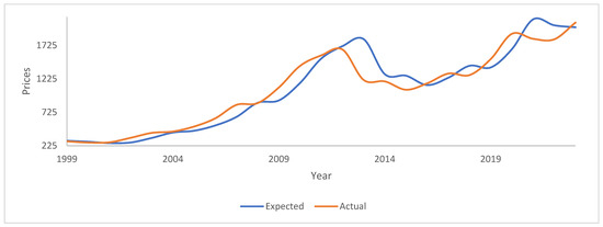
Figure 1.
Expected and actual gold prices at an annual frequency. The figure plots the actual vs. the expected prices at an annual frequency. The prices on the y-axis are the actual and expected prices. The expected price is obtained using the manuscript’s methodological procedure.
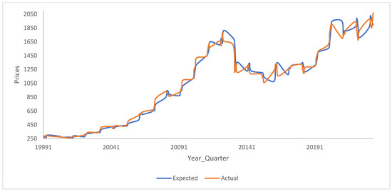
Figure 2.
Expected and actual gold prices at a quarterly frequency. The figure plots the actual vs. the expected prices at a quarterly frequency. The prices on the y-axis are the actual and expected prices. The expected price is obtained using the manuscript’s methodological procedure.
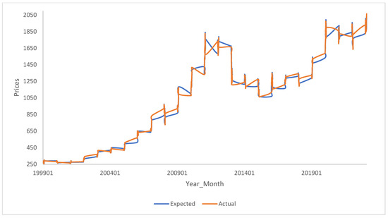
Figure 3.
Expected and actual gold prices at a monthly frequency. The figure plots the actual vs. the expected prices at a monthly frequency. The prices on the y-axis are the actual and expected prices. The expected price is obtained using the manuscript’s methodological procedure.
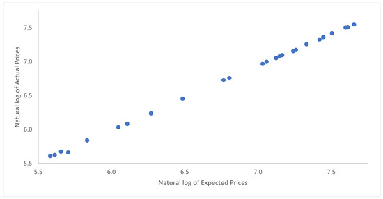
Figure 4.
Expected vs. actual gold prices at an annual frequency. This figure plots the natural logarithms of the observed prices (y-axis) against the natural logarithms of the expected prices (x-axis) estimated using the manuscript’s methodology at an annual frequency.
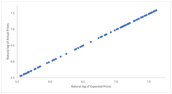
Figure 5.
Expected vs. actual gold prices at a quarterly frequency. This figure plots the natural logarithms of the observed prices (y-axis) against the natural logarithms of the expected prices (x-axis) estimated using the manuscript’s methodology at a quarterly frequency.
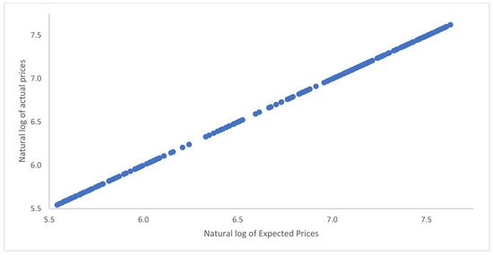
Figure 6.
Expected vs. actual gold prices at a monthly frequency. This figure plots the natural logarithms of the observed prices (y-axis) against the natural logarithms of the expected prices (x-axis) estimated using the manuscript’s methodology at a monthly frequency.
The efficacy of using the GBM simulated expected price to predict the actual gold prices was tested using a simple regression, shown in Equation (11). In this equation, Pt,actual is the actual gold price at the end of a period, while Pt,exp is the GBM-simulated expected price for that period. α is the intercept, while β is the slope coefficient. The regression error term is represented by In Equation (11), the natural logarithms of both the actual and the expected prices are used in the regressions. This equation can be used to test whether the expected price is a good reliable forecast of the actual price. Alternatively, it could also be used as a predictive model for the actual price using the expected price as the independent variable. Values of 0 for α and one for β would indicate the usefulness of the expected price. A similar logic was used in Refs. [18,32,33] as well as by Ref. [37] who tested the persistence of mutual fund performance between two adjacent periods. The regression represented in Equation (11) was carried out at annual, quarterly, and monthly frequencies in our study, and the results are presented in Table 2.
Table 2.
Regression results.
The usefulness of the GBM-simulated expected gold prices as predictors of the actual prices was also tested to check if the means and variances between the two were different. The two price series—the natural logarithms of the observed prices and those of the expected prices—were first tested for differences in terms of variances. The difference in variance between the two series was hypothesized to be zero, and the F-stat was estimated using Equation (12). The averages of the natural logarithms of the observed and estimated prices were also tested using the two-sample t-stat estimated using pooled variances. The formulas for the pooled variances and the t-stats are represented in Equations (13) and (14), respectively. The formulas from Equations (12)–(14) can be found in most statistical textbooks, like Ref. [38]. A t-stat test was conducted assuming equal variances after the F-stat test for variances that did not reject the hypothesis of no differences in terms of variance. In Equations (13) and (14), n1 = n2, and the difference between the two means, (µ1–µ2), is hypothesized to not be different from zero. Table 3 presents the results of these tests.
Table 3.
Testing the means and variances.
4. Results
Figure 1, Figure 2 and Figure 3 are plots of the expected and actual prices against time. In these figures, the actual USD prices are used. Figure 1 shows the annual frequency, while Figure 2 reflects the quarterly frequency and Figure 3 the monthly frequency. Very strong correlations between the observed and expected prices are observed in each of the three figures. Numerically and as presented in the figures, the actual prices are sometimes above the expected prices, while, at other times, it is the other way around. Nevertheless, the two lines are very close and move closer to each other as we move from the annual to the monthly frequency. Figure 4, Figure 5 and Figure 6 are plots of the natural logarithms of the observed prices against the natural logarithms of the expected prices. All three plots show upward-sloping straight lines, indicating a strong possibility of a linear relationship between the actual and expected prices. Perhaps, the expected prices obtained using the manuscript’s methodology can serve as good proxies of the actual prices or at least help in making reliable forecasts of the actual prices of gold.
Table 2 presents the results of the simple regression in Equation (11). The results are presented for all three frequencies. The values of the intercept are close to zero. At the annual frequency, the value of the intercept is equal to 0.3, but, for the quarterly and annual frequencies, it is 0.08 and 0.03, respectively. Statistically, primarily based on the t-stats, the hypothesis that the coefficient of the independent variable are not equal to zero cannot be rejected, primarily because the standard errors for the intercept terms are very small. The values of the coefficient for the annual, quarterly, and monthly frequencies are 0.95, 0.99, and 0.99 when rounded-off to two decimal places. The hypothesis that the coefficients are non-zero values cannot be rejected at the one percent significance level. They are also different from a value of one, given the very low values obtained for their standard errors. For all three regressions, the adjusted R-square and the R-square are very high. Given the model’s characteristics and the significance level of the t-stats, the expected values can be used to predict the actual gold prices.
The results for the testing of the averages and variances of the natural logarithms of the estimated price and the observed gold prices are presented in Table 3. In our study, the tests for differences in the variances have been carried out before the tests for differences in the means. The F-stat, as estimated by Equation (12), shows values of 1.11, 1.03, and 1.01 at the yearly, quarterly, and monthly frequencies. The table below also presents the critical F-values at these frequencies, and it can be observed that the test’s statistics are less than the critical F-stat. The hypothesis that there is no difference in terms of the variances in the natural logarithms of the estimated prices and the natural logarithms of the observed prices cannot be rejected. Given that the hypothesis cannot be rejected, the difference in the means of the two price series are tested assuming no differences in the variances. The test’s statistic is a t-stat, estimated, as shown in Equation (14), using the pooled variance estimated using Equation (13). The pooled variances, test statistics, critical value of the test statics, as well as the p-values are presented in Table 3. The t-stat test statistics are 0.27, 0.14, and 0.08 at the annual, quarterly, and monthly frequencies. The p-values are also higher than the normally used alpha of 5%. The hypothesis, as far as the natural logarithms of the estimated price and the natural logarithms of the actual prices are concerned, that their averages are not different from one another cannot be rejected. Thus, at least statistically speaking, there is no difference between the average and variance of the natural logarithms of the GBM-simulated gold prices and those of the actually observed gold prices at yearly, quarterly, and monthly frequencies.
5. Conclusions
Gold objects have been of prime importance for a very long time [1,2,3], and gold itself has gathered importance as a hedging instrument [4,5,6] as well. Given the growing importance of gold, gold prices are a subject of renewed interest [7] for a large number of economic entities. Accordingly, a number of researchers have developed and tested models to obtain gold prices, such as Refs. [8,9,10,39,40], among others. Ref. [8] applied a number of different time series models to obtain gold prices from Thailand, at a monthly frequency, between 2009 and 2021. Ref. [9] applied the ARIMA model to forecast gold prices based on monthly data obtained from the Multi Commodity Exchange of India for the period between 2003 and 2014. Ref. [10] applied a multivariate stochastic model to predict gold prices. Ref. [39] found the ARIMA approach to provide good forecasts, after comparing six different estimating procedures typically used to forecast gold prices and the prices of other metals like silver, platinum, palladium, and rhodium. Ref. [40] applied the exponential-smoothing approach to predict Malaysian monthly gold prices from data obtained from the World Bank. The GBM approach can be found among the popular methods for obtaining accurate forecasts, a method which has also been used to forecast the prices of a number of different assets like stocks, stock indices, options, energy products, agricultural products, and metals, including gold.
In this manuscript, a GBM approach was used to obtain accurate and reliable gold prices. While GBM has also been used to assess gold prices in Refs. [11,12,13], the methodology used in this manuscript is similar that used in Refs. [18,32,33]. Using GBM, one hundred thousand one-period-ahead prices and returns of gold were obtained at yearly, quarterly, and monthly frequencies. From the simulated returns, probabilities were obtained by taking the differences in the cumulative distribution function of two adjacent returns after the returns had been sorted from low to high. By multiplying simulated prices with the associated probabilities, and adding up the such multiplication, the expected prices were obtained. Results indicated that the expected prices can be good and reliable predictors of the actual prices. The averages and variances of the natural logarithms of the estimated prices were also found to be similar to those of the actually observed prices.
Funding
This research received no external funding.
Institutional Review Board Statement
Not applicable.
Informed Consent Statement
Not applicable.
Data Availability Statement
No new data was created. Data was obtained from DataStream through a subscription from Refinitiv.
Conflicts of Interest
The author declares no conflicts of interest.
References
- Erb, C.B.; Harvey, C.R. The Golden Dilemma. SSRN Electron. J. 2012, 69, 10–42. [Google Scholar] [CrossRef][Green Version]
- Beckmann, J.; Czudaj, R. Gold as an inflation hedge in a time-varying coefficient framework. N. Am. J. Econ. Financ. 2013, 24, 208–222. [Google Scholar] [CrossRef]
- Mukul, M.K.; Kumar, V.; Ray, S. Gold ETF Performance: A Comparative Analysis of Monthly Returns Gold ETF Performance: A Comparative Analysis of Monthly Returns. IUP J. Financ. Risk Manag. 2012, 9, 59–63. [Google Scholar]
- Erb, C.B.; Harvey, C.R. An Impressionistic View of the “Real” Price of Gold Around the World. SSRN Electron. J. 2012, 2012, 2148691. [Google Scholar] [CrossRef]
- Erb, C.B.; Harvey, C.R. The Golden Constant. SSRN Electron. J. 2015, 26, 94–101. [Google Scholar] [CrossRef]
- Reboredo, J.C. Is gold a safe haven or a hedge for the US dollar? Implications for risk management. J. Bank. Financ. 2013, 37, 2665–2676. [Google Scholar] [CrossRef]
- Shafiee, S.; Topal, E. An overview of global gold market and gold price forecasting. Resour. Policy 2010, 35, 178–189. [Google Scholar] [CrossRef]
- Jetwanna, K.W.; Choksuchat, C.; Matayong, S.; Prateepausanont, N.; Wiwattanasaranrom, U. Utilization of various time series models forecasting gold prices in Thailand. Sci. Eng. Health Stud. 2023, 17, 23020007. [Google Scholar]
- Guha, B.; Bandyopadhyay, G. Gold Price Forecasting Using ARIMA Model. J. Adv. Manag. Sci. 2016, 4, 117–121. [Google Scholar] [CrossRef]
- Madziwa, L.; Pillalamarry, M.; Chatterjee, S. Gold price forecasting using multivariate stochastic model. Resour. Policy 2022, 76, 102544. [Google Scholar] [CrossRef]
- Roslan, N.H.A.; Halim, N.A. Forecasting World Gold Price in Year 2022 Using Geometric Brownian Motion Model. In Proceedings of the 29th National Symposium on Mathematical Sciences, Virtual, 7–8 September 2022; p. 050003. [Google Scholar]
- Germansah, G.; Tjahjana, R.H.; Herdiana, R. Geometric Brownian Motion in Analyzing Seasonality of Gold Derivative Prices. Eduvest J. Univers. Stud. 2023, 3, 1558–1572. [Google Scholar] [CrossRef]
- Hamdan, Z.N.; Ibrahim, S.N.I.; Mustafa, M.S. Modelling malaysian gold prices using geometric brownian motion model. Adv. Math. Sci. J. 2020, 9, 7463–7469. [Google Scholar] [CrossRef]
- Bachelier, L. Théorie de la Spéculation; Gauther Villar: Paris, France, 1900. [Google Scholar]
- Samuelson, P.A. Rational Theory of Warrant Pricing. Ind. Manag. Rev. 1965, 6, 13–39. [Google Scholar]
- Samuelson, P.A. Mathematics of Speculative Price. SIAM Rev. 1973, 15, 1–42. [Google Scholar] [CrossRef]
- Shehzad, H.T.; Anwar, M.A.; Razzaq, M. A Comparative Predicting Stock Prices using Heston and Geometric Brownian Motion Models. arXiv 2023, arXiv:2302.07796. [Google Scholar]
- Sinha, A.K. The reliability of geometric Brownian motion forecasts of S&P500 index values. J. Forecast. 2021, 40, 1444–1462. [Google Scholar] [CrossRef]
- Black, F.; Scholes, M. The Pricing of Options and Corporate Liabilities. J. Polit. Econ. 1973, 81, 637. [Google Scholar] [CrossRef]
- Croghan, J.; Jackman, J.; Min, K.J. Estimation of Geometric Brownian motion Parameters for Oil Price Analysis. In Proceedings of the 67th Annual Conference and Expo of the Institute of Industrial Engineers 2017, New Orleans, LA, USA, 30 May–2 June 2020; pp. 1858–1863. [Google Scholar]
- Chan, J.C.C.; Grant, A.L. Modeling energy price dynamics: GARCH vs. stochastic volatility. Energy Econ. 2016, 54, 182–189. [Google Scholar] [CrossRef]
- Ibrahim, S.N.I.; Misiran, M.; Laham, M.F. Geometric fractional Brownian motion model for commodity market simulation. Alex. Eng. J. 2021, 60, 955–962. [Google Scholar] [CrossRef]
- Ibrahim, S.N.I. Modeling Rubber Prices as a GBM Process. Indian J. Sci. Technol. 2016, 9, 1–6. [Google Scholar] [CrossRef]
- Ramos, A.L.; Mazzinghy, D.B.; Barbosa, V.D.S.B.; Oliveira, M.M.; da Silva, G.R. Evaluation of an iron ore price forecast using a geometric brownian motion model. Rev. Esc. Minas 2019, 72, 9–15. [Google Scholar] [CrossRef][Green Version]
- Inci, A.C.; Lu, B. Exchange rates and interest rates: Can term structure models explain currency movements? J. Econ. Dyn. Control. 2004, 28, 1595–1624. [Google Scholar] [CrossRef]
- Alhagyan, M. The effects of incorporating memory and stochastic volatility into GBM to forecast exchange rates of Euro. Alex. Eng. J. 2022, 61, 9601–9608. [Google Scholar] [CrossRef]
- Benninga, S.; Mofkadi, T. Financial Modeling, 5th ed.; MIT Press: Cambridge, MA, USA, 2021. [Google Scholar]
- Benninga, S. Financial Modeling, 4th ed.; MIT Press: Cambridge, MA, USA, 2014; ISBN 9780262027281. [Google Scholar]
- Hull, J. Options, Futures, and Other Derivatives, 10th ed.; Pearson: London, UK, 2018; ISBN 978-0134472089. [Google Scholar]
- Musiela, M.; Rutkowski, M. Martingale Methods in Financial Modelling. In Stochastic Modelling and Applied Probability; Springer: Berlin/Heidelberg, Germany, 2005; Volume 36, ISBN 978-3-540-20966-9. [Google Scholar]
- Navin, R.L. The Mathematics of Derivatives: Tools for Designing Numerical Algorithms; John Wiley & Sons, Inc: Hoboken, NJ, USA, 2007; ISBN 978-0-470-04725-5. [Google Scholar]
- Sinha, A.K. Do Economic and Financial Factors Affect Expected S&P 500. In Selected Topics in Econophysics; Sinha, A.K., Ed.; De Gruyter Academic Publishing: Berlin, Germany, 2024. [Google Scholar]
- Sinha, A.K. Simplifying to Improve Reliability of Geometric Brownian Motion Stock Index Forecasts. In Selected Topics in Econophysics; Sinha, A.K., Ed.; De Gruyter Academic Publishing: Berlin, Germany, 2024. [Google Scholar]
- Sengupta, C. Financial Modeling Using Excel and VBA; John Wiley & Sons, Inc: Hoboken, NJ, USA, 2004; ISBN 0471267686,9780471267683. [Google Scholar]
- Estember, R.D.; Maraña, M.J.R. Forecasting of Stock Prices Using Brownian Motion-Monte Carlo Simulation. In Proceedings of the International Conference on Industrial Engineering and Operations Management, Kuala Lumpur, Malaysia, 8–10 March 2016; Volume 8–10. [Google Scholar]
- Urama, T.C.; Ezepue, P.O. Stochastic Ito-Calculus and Numerical Approximations for Asset Price Forecasting in the Nigerian Stock Market. J. Math. Financ. 2018, 08, 640–667. [Google Scholar] [CrossRef][Green Version]
- Grinblatt, M.; Titman, S. The Persistence of Mutual Fund Performance. J. Financ. 1992, 47, 1977–1984. [Google Scholar] [CrossRef]
- Berenson, M.L.; Levine, D.M.; Krehbiel, T.C. Basic Business Statistics: Concepts and Applications, 11th ed.; Pearson Prentice Hall: London, UK, 2015; ISBN 9780136034384. [Google Scholar]
- Azzutti, A. Forecasting Gold Price: A Comparative Study. Course Financ. Econ. Univ. Florence 2016. [Google Scholar] [CrossRef]
- Rahman, H.A.A.; Azizi, M.F.R.; Saruand, M.F.; Shafie, N.A. Forecasting of Malaysia Gold Price with Exponential Smoothing. J. Sci. Technol. 2022, 14, 44–50. [Google Scholar] [CrossRef]
Disclaimer/Publisher’s Note: The statements, opinions and data contained in all publications are solely those of the individual author(s) and contributor(s) and not of MDPI and/or the editor(s). MDPI and/or the editor(s) disclaim responsibility for any injury to people or property resulting from any ideas, methods, instructions or products referred to in the content. |
© 2024 by the author. Licensee MDPI, Basel, Switzerland. This article is an open access article distributed under the terms and conditions of the Creative Commons Attribution (CC BY) license (https://creativecommons.org/licenses/by/4.0/).