Copula-Based Bayesian Model for Detecting Differential Gene Expression

Abstract

Deoxyribonucleic acid, more commonly known as DNA, is a fundamental genetic material in all living organisms, containing thousands of genes, but only a subset exhibit differential expression and play a crucial role in diseases. Microarray technology has revolutionized the study of gene expression, with two primary types available for expression analysis: spotted cDNA arrays and oligonucleotide arrays. This research focuses on the statistical analysis of data from spotted cDNA microarrays. Numerous models have been developed to identify differentially expressed genes based on the red and green fluorescence intensities measured using these arrays. We propose a novel approach using a Gaussian copula model to characterize the joint distribution of red and green intensities, effectively capturing their dependence structure. Given the right-skewed nature of the intensity distributions, we model the marginal distributions using gamma distributions. Differentially expressed genes are identified using the Bayes estimate under our proposed copula framework. To evaluate the performance of our model, we conduct simulation studies to assess parameter estimation accuracy. Our results demonstrate that the proposed approach outperforms existing methods reported in the literature. Finally, we apply our model to Escherichia coli microarray data, illustrating its practical utility in gene expression analysis.

1. Introduction

Microarray technology is a cutting-edge approach to gene expression analysis, widely used in fields such as basic biology and medical science. Over the past two decades, the number of gene expression studies employing microarrays has grown rapidly. Two primary microarray technologies are available for expression analysis: spotted cDNA arrays and oligonucleotide arrays. While our research primarily focuses on the statistical analysis of data from spotted cDNA microarrays, the methods discussed here can be adapted for data generated via Affymetrix chips. In microarray experiments, RNA is first extracted from the subject cells. Some of its molecules are then replaced with counterparts containing a fluorescent dye, producing labeled transcripts known as targets. In cDNA microarrays, both targets and probes are cDNA molecules, whereas, in oligonucleotide arrays, the targets remain cDNA molecules, but the probes consist of carefully selected small cDNA segments known as oligos.

A cDNA microarray is commonly referred to as a two-channel array. In this technology, both an experimental sample and a reference sample are labeled with fluorescent dyes—Cyanine 3 (Cy3, green) and Cyanine 5 (Cy5, red)—on a single chip, with the experimental sample typically labeled with Cy5 [1]. Each chip contains thousands of spots, each corresponding to a specific gene. A laser microscope scanner measures the fluorescence intensity at each spot, providing a quantitative assessment of gene expression. Colored spots indicate genes expressed in one or both samples, while gray areas represent genes not expressed in either sample. Although microarray data capture thousands of genes, only a subset of differentially expressed genes (DEGs) may be biologically significant, particularly in diseases such as cancer. Therefore, identifying these DEGs is a crucial step in microarray analysis. Numerous methods have been proposed in the literature to detect differentially expressed genes.

The fold-change method was one of the earliest techniques used in microarray data analysis [2,3,4]. This simple approach identifies differentially expressed genes (DEGs) by applying a predefined threshold on fold change. However, it is prone to bias, particularly when the data are not properly normalized [5]. Moreover, since it does not account for statistical variation, the method is considered unreliable. To address these limitations, later approaches incorporated the probabilistic modeling of red (R) and green (G) intensities for DEG detection. These methods established classification rules based on distributional assumptions of $(R,G)$. For example, ref. [6] proposed a data-driven threshold selection for the ratio $R/G$, assuming normality and a constant coefficient of variation. However, a key drawback of this approach is that it overlooks the valuable information contained in the product $RG$.

To avoid this problem, ref. [7] suggested a hierarchical model (Gamma–Gamma–Bernoulli) to capture DEGs based on the posterior odds of change (the odds are functions of $R+G$ and $RG$). This method assumes that R and G are independent. Mav and Chaganty [8] have shown that the R and G are positively correlated. They have built a bivariate distribution with gamma marginals and a positive correlation between R and G to incorporate this dependence. They also incorporated a latent Bernoulli variable. They used the EM algorithm to calculate the posterior probabilities of differential expression. The DEGs are the ones with higher posterior probabilities.

A Bayesian approach to testing multiple hypotheses in microarray experiments was proposed by Maria et al. (2020) [9], pointing to the use of copula functions to model dependence. Their method demonstrated that incorporating dependency structures significantly improves classification accuracy when identifying differentially expressed genes. The term “copula” was first used by Sklar in 1959 [10]; its meaning is that it “ties” the marginal uniform distributions to create a joint distribution function. An excellent introduction to copulas is the book by Nelsen [11]. Copula functions are useful for constructing bivariate or, in general, multivariate distributions with given marginal distributions. Since their introduction, the literature and applications of copulas have grown rapidly. Some classic books on the topic include [11,12]. More comprehensive coverage of copula models and their applications is given in [13].

Over the past decade, extensive research has explored the application of copulas in genomics, particularly for analyzing gene expression data. For instance, Chaba (2017) [14] proposed a semi-parametric copula-based approach to differential gene expression analysis. Likewise, Ray et al. (2020) [15] introduced a copula-based model that focuses on detecting differential co-expression, rather than differential expression, emphasizing the significance of dependency structures in gene networks.

Although copulas are increasingly used in gene expression studies, existing approaches have not been specifically developed to detect differentially expressed genes in microarray experiments. To address this gap, we introduce a copula-based framework particularly for DEG detection, utilizing copulas to model dependencies between gene intensities while offering a probabilistic basis for differential expression analysis. In this article, we extend the work done by Mav and Chaganty [8], replacing the joint probability distribution of red and green intensities with a Gaussian copula-based joint distribution. The DEGs can be identified by calculating the Bayes estimate of the differential expression under this model.

The outline of the article is as follows. Section 2 describes the challenges in analyzing microarray data and the need for sophisticated statistical models to accurately capture the dependence structure between gene expressions. The theoretical foundation of the copula model, including the formulation of the model and the specification of prior distributions for the parameters, is explained in Section 3.

In Section 4, we present the methodology for estimating the parameters of the copula model using maximum likelihood estimation and Bayesian inferential procedures. The section also details the numerical optimization routines employed. Section 4 provides an in-depth discussion of the estimation process, including the steps involved in maximizing the log-likelihood function and implementing the quasi-Newton algorithm. Section 5 focuses on identifying differentially expressed genes using the estimated copula model parameters and explaining the statistical tests and criteria used. In Section 6, we explore the relationship between the copula parameter and the correlation coefficient, providing insights into how the copula model captures dependencies between gene expression levels.

Section 7 presents the results of simulation studies conducted to evaluate the performance of the copula-based Bayesian model in identifying differentially expressed genes and comparing it with other existing methods. Section 8 contains the application of the copula-based Bayesian model to real datasets of gene expression levels in Escherichia coli, demonstrating the practical utility of the model. Finally, by comparing the log-likelihood values, we show that this Gaussian copula model improves over the models given in [7,8].

2. Motivation

Escherichia coli (E. coli) is a bacteria that generally lives in the intestines of people and animals. The motivating data for this article is the experiment designed to study gene expression levels in E. coli, described in [16]. The E. coli genome consists of approximately 4.6 million base pairs (Mbp), but it is suspected of encoding only about forty-two hundred genes. To study differential gene expressions in E. coli, ref. [16] used two traditional treatments that affect gene expression levels. The first treatment was induction with isopropyl-$\beta$-D-thiogalactopyranoside (IPTG), which tests the methods since only a few gene transcripts are expected to change. Secondly, heat shock treatment allows global regulatory effects to be observed. A single colony of E. coli K-12 was divided into five samples for the experiments.

IPTG treatment was performed independently on two samples (IPTG-A and IPTG-B), while one sample (control) was untreated. Heat shock induction was carried out by treating the culture to a 50 °C shaking water bath for seven minutes on the remaining two samples (Heat Shock A and Heat Shock B). Following the hybridization of the samples on E. coli microarrays, the signal intensities for each spot were determined using the ScanAlyze software 1.0.3. The average fluorescence intensity for each spot was measured, and the background was chosen as the median pixel intensity in a square surrounding each spot. The red and green signal intensities were recalculated and normalized after background subtraction.

Newton et al. [7] proposed a Bayesian hierarchical model with a latent variable to identify differentially expressed genes. In their approach, the marginal distributions of red and green intensities were modeled as gamma distributions with common shape parameters but different scale parameters. However, they assumed that the red and green intensities for the same gene were independent. To address this limitation, Mav and Chaganty [8] introduced a bivariate distribution with gamma marginals that incorporated a positive correlation between the red and green intensities. In this article, we extend their approach by replacing the bivariate distribution with a bivariate Gaussian copula, constructing a joint distribution with gamma marginals. The performance of our proposed model is evaluated through log-likelihood analysis using E. coli data.

3. Copula-Based Bayesian Model for Expression Level

The typical objective when analyzing data from microarray experiments is to identify differentially expressed genes. This section will propose a copula-based Bayesian model that can filter these genes. Consider a microarray consisting of n genes. Let $R_{1j}$ and $R_{2j}$ denote the red and green intensities of gene j, respectively. The concepts based on the red and green intensity ratio have been widely used in the literature to identify differentially expressed genes. Some of those were discussed briefly in Section 1. To filter the differentially expressed genes, we will use the ratio of expected expression levels, which are given by ${\eta }_j=E\left(R_{1j}\right)/E\left(R_{2j}\right)$, where E stands for the expected value.

As explained in Section 2, this study was motivated by E. coli data. Gamma distribution has been widely used in statistical analysis in microarray experiments [17,18,19], not only for its analytical convenience but also for its ability to be interpreted in a deeper way. The family of gamma distributions is supported on the positive line and provides a rich class of distributions as special cases [17]. In addition, Chen et al. in 1997 [6] presented an intriguing argument that, while expected expression levels vary from gene to gene in the microarray, the measurements are connected via a constant coefficient of variation ($CV$) and $CV=1/\alpha$. Having a common shape parameter, $\alpha$, ensures that the variability structure remains consistent across genes and makes it convenient to model the variability in gene expression. Taking into account all of the above facts, we assume $R_{ij}$ and $R_{2j}$ are gamma distributions with a common shape parameter, $\alpha$, but different scale parameters, $1/{\theta }_{1j}$ and $1/{\theta }_{2j}$ for $j=1,2,\dots ,n$. The probability density function of $R_{ij}$ is given by

$$\begin{array}{ccc}\hfill f_i(r_{ij};{\theta }_{ij},\alpha )& =& {\displaystyle \frac{1}{\Gamma \left(\alpha \right)}{\theta }_{ij}^{\alpha }{r}_{ij}^{\alpha -1}exp(-{\theta }_{ij}{r}_{ij}),i=1,2;j=1,\dots ,n.}\hfill \end{array}$$

(1)

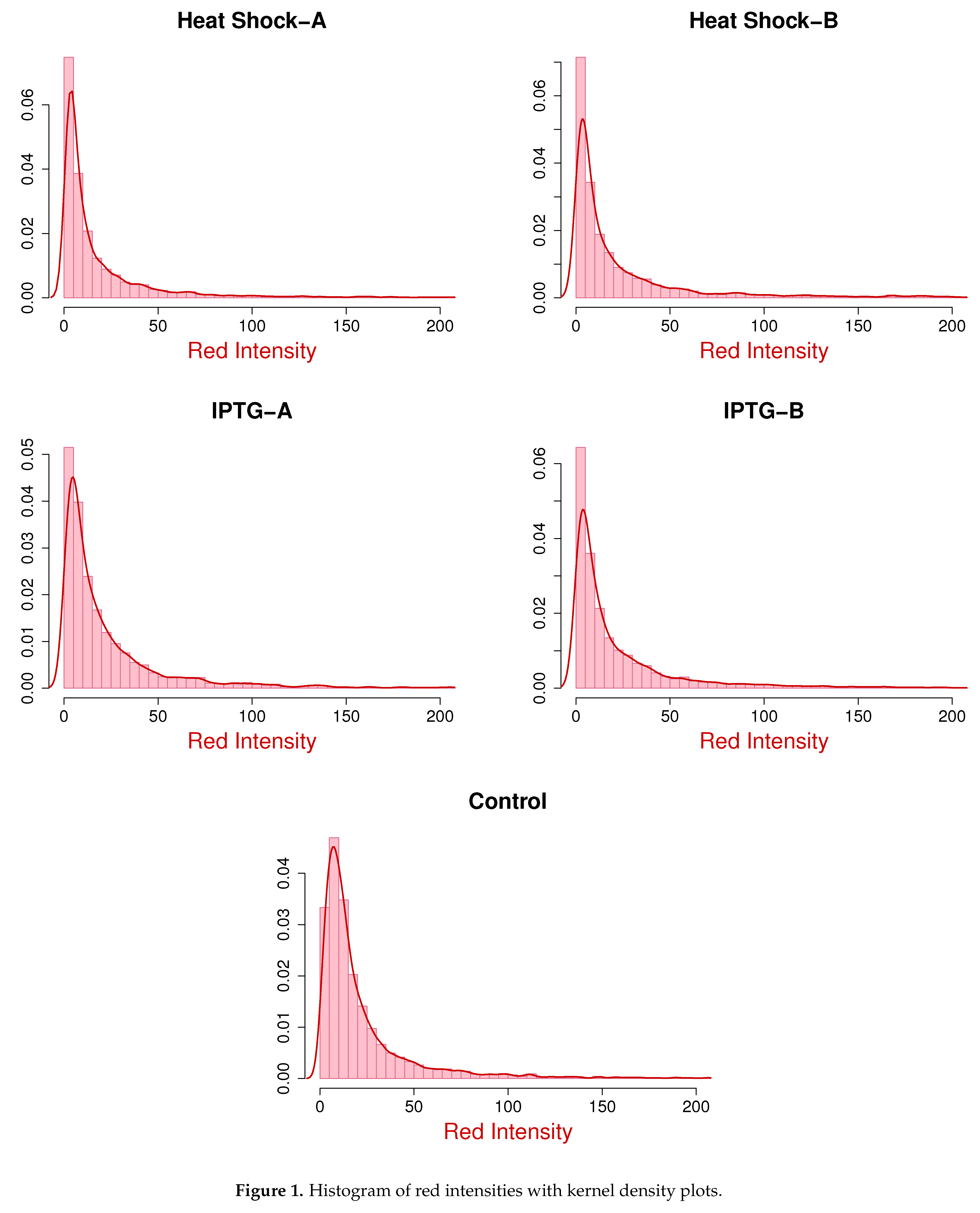
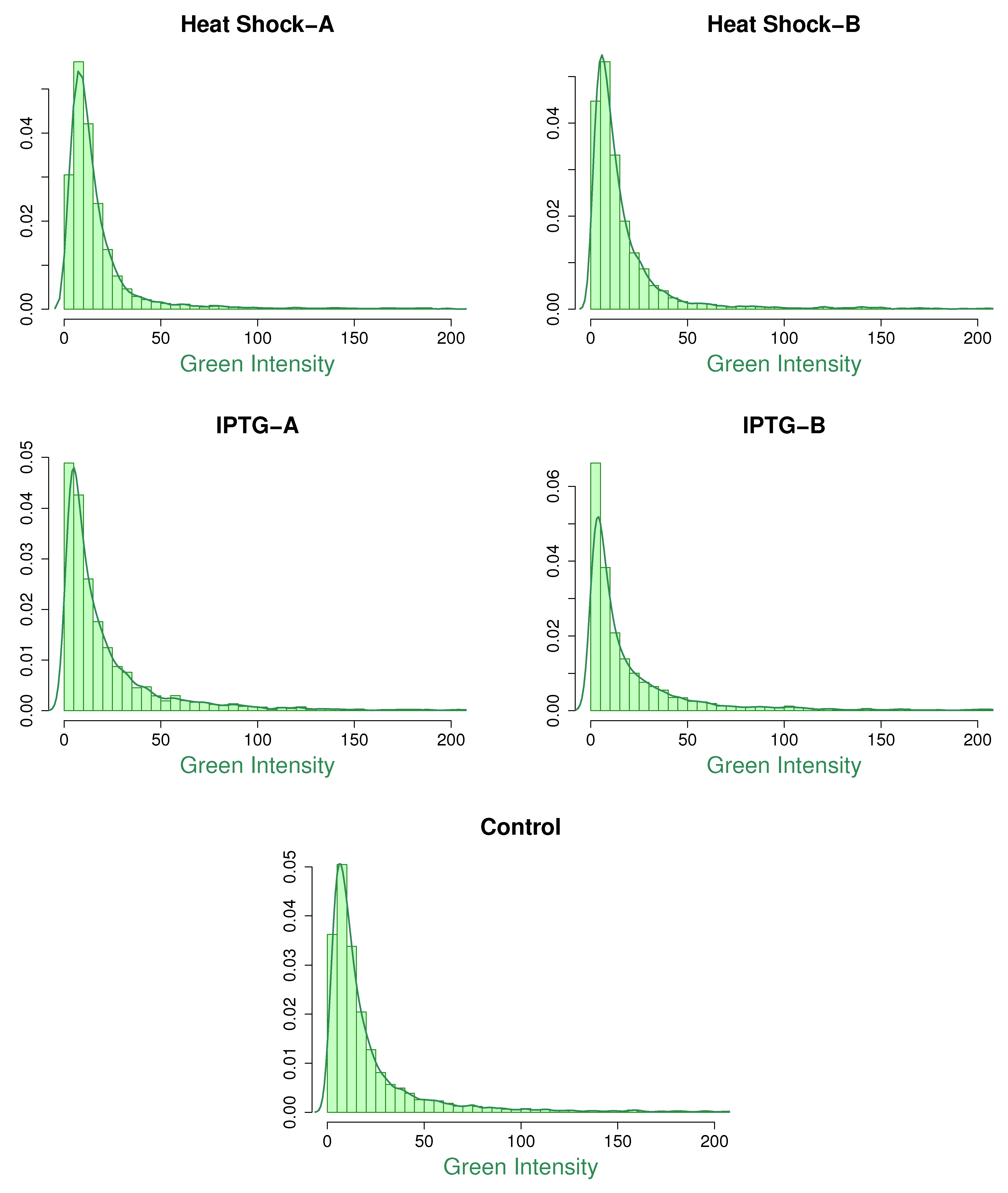
Figure 1 and Figure 2 show the histograms of red and green intensities along with nonparametric kernel density plots for the five microarray experiments. The positively skewed shape of the density curves suggests that the assumption of gamma marginals is reasonable. Note that $E\left(R_{ij}\right)=\alpha /{\theta }_{ij}$ for $i=1,2$. Therefore, the ratio of expected expression levels ${\eta }_j=E\left(R_{1j}\right)/E\left(R_{2j}\right)={\theta }_{2j}/{\theta }_{1j}$ for $j=1,\dots ,n$. To model the dependence between the two intensities, we assume the joint distribution of $(R_{1j},R_{2j})$ is given by the bivariate Gaussian copula and can be written as

$$\begin{array}{ccc}\hfill f(r_{1j},r_{2j};{\theta }_{1j},{\theta }_{2j},\alpha ,\gamma )& =& c(u_{1j},u_{2j};\gamma )f_1\left(r_{1j}\right)f_2\left(r_{2j}\right),\hfill \end{array}$$

(2)

where $u_{ij}=F_i\left(r_{ij}\right)$ and $F_i(.)$ is the cumulative distribution function of a gamma distribution with parameters $(\alpha ,1/{\theta }_{ij})$. Note that the Gaussian copula density is

$$\begin{array}{ccc}\hfill c(u_{1j},u_{2j};\gamma )& =& {\displaystyle \frac{1}{\sqrt{1-{\gamma }^2}}exp\left[-\frac{1}{2}\left(\frac{{\gamma }^2(z_{1j}^2+z_{2j}^2)-2\gamma z_{1j}{z}_{2j}}{1-{\gamma }^2}\right)\right],}\hfill \end{array}$$

(3)

where $z_{ij}={\Phi }^{-1}\left(u_{ij}\right)$, and $\gamma$ is the parameter of the copula density. To simplify the notation moving forward, we write $c(u_{1j},u_{2j})$ in place of $c(u_{1j},u_{2j};\gamma )$.

The joint distribution in (2) consists of $2n+2$ unknown parameters. Since there are too many unknown parameters, we adopt the empirical Bayes approach to make the model parsimonious. This requires specification of prior distributions for the gene-specific parameters ${\theta }_{1j}$ and ${\theta }_{2j}$. We assume independent gamma distributions with parameters ${\alpha }_0$ and $1/\nu$ as the prior distributions for ${\theta }_{ij}$.

The prior density $\pi \left({\theta }_{ij}\right)$ is

$$\begin{array}{ccc}\hfill \pi ({\theta }_{ij};\nu ,{\alpha }_0)& =& {\displaystyle \frac{1}{\Gamma \left({\alpha }_0\right)}{\nu }^{{\alpha }_0}{\theta }_{ij}^{{\alpha }_0-1}exp(-\nu {\theta }_{ij}),\mathrm{for}i=1,2;j=1,\dots ,n.}\hfill \end{array}$$

(4)

Multiplying (2) and (4), we get the joint density of $(R_{1j},R_{2j})$ and $({\theta }_{1j},{\theta }_{2j})$ as

$$\begin{array}{ccc}\hfill f(r_{1j},r_{2j},{\theta }_{1j},{\theta }_{2j};\mathbf{{\rm Y}})& =& {\left({\displaystyle \frac{{\nu }^{{\alpha }_0}}{\Gamma \left(\alpha \right)\Gamma \left({\alpha }_0\right)}}\right)}^{2}c(u_{1j},u_{2j})\prod _{i=1}^2\left[{\displaystyle r_{ij}^{\alpha -1}{\theta }_{ij}^{\alpha +{\alpha }_0-1}exp(-{\theta }_{ij}(r_{ij}+\nu ))}\right],\hfill \end{array}$$

(5)

where $\mathbf{{\rm Y}}=(\alpha ,{\alpha }_0,\nu ,\gamma )$ is the vector of model parameters. Recall that this model has gene-specific parameters, $({\theta }_{1j},{\theta }_{2j})$, for $j=1,\dots ,n$. The marginal density of ${\mathbf{R}}_j=(R_{1j},R_{2j})$ is

$$\begin{array}{ccc}\hfill f_m(r_{1j},r_{2j};\mathbf{{\rm Y}})& =& {\int }_0^{\infty }{\int }_0^{\infty }f(r_{1j},r_{2j};{\theta }_{1j},{\theta }_{2j};\mathbf{{\rm Y}})d{\theta }_{1j}d{\theta }_{2j}\hfill \\ \hfill \\ & =& {\left({\displaystyle \frac{{\nu }^{{\alpha }_0}}{\Gamma \left(\alpha \right)\Gamma \left({\alpha }_0\right)}}\right)}^2{\int }_0^{\infty }{\int }_0^{\infty }c(F_1\left(r_{1j}\right),F_2\left(r_{2j}\right))\times \hfill \\ \hfill \\ & & \prod _{i=1}^2\left[{\displaystyle r_{ij}^{\alpha -1}{\theta }_{ij}^{\alpha +{\alpha }_0-1}exp(-{\theta }_{ij}(r_{ij}+\nu ))}\right]d{\theta }_{1j}d{\theta }_{2j}.\hfill \end{array}$$

(6)

Here, $F_i\left(r_{ij}\right)$ is the cumulative distribution function of gamma with parameters $\alpha$ and $1/{\theta }_{ij}$ for $i=1,2$ and $j=1,2,\dots ,n$.

The double integral in Equation (6) does not simplify because of the presence of the Gaussian copula function $c(u_{1j},u_{2j})$ in the integrand. A numerical computation of the double integral (6) is also challenging. To compute the double integral, we could use the R libraries, such as the cubature by [20] or pracma by [21]. We were unsuccessful with these packages and encountered numerous errors with the functions embedded in these packages when evaluating the double integral iteratively. To overcome the computational problems, we have developed our own R code to evaluate the double integral and obtain the marginal density of ${\mathbf{R}}_j=(R_{1j},R_{2j})$.

4. Parameter Estimation Procedure

The marginal bivariate density of red and green intensities given in (6) has four unknown parameters given by the vector $\mathbf{{\rm Y}}=(\alpha ,{\alpha }_0,\nu ,\gamma )$. Maximum likelihood is the most efficient method for estimating these parameters. This method entails maximizing the likelihood or the log-likelihood, which is the logarithm of the likelihood function. For n genes, the log-likelihood is given by

$$\begin{array}{ccc}\hfill l\left(\mathbf{{\rm Y}}\right)& =& \sum _{j=1}^{n}log{f}_m(r_{1j},r_{2j};\mathbf{{\rm Y}})\hfill \\ \hfill \\ & =& \sum _{j=1}^{n}log[{\left({\displaystyle \frac{{\nu }^{{\alpha }_0}}{\Gamma \left(\alpha \right)\Gamma \left({\alpha }_0\right)}}\right)}^2{\int }_0^{\infty }{\int }_0^{\infty }c(F_1\left(r_{1j}\right),F_2\left(r_{2j}\right))\times \hfill \\ \hfill \\ & & \prod _{i=1}^2\left[{\displaystyle r_{ij}^{\alpha -1}{\theta }_{ij}^{\alpha +{\alpha }_0-1}exp(-{\theta }_{ij}(r_{ij}+\nu ))}\right]d{\theta }_{1j}d{\theta }_{2j}]\hfill \\ \hfill \\ & =& 2n\left[{\alpha }_{0}log\left(\nu \right)-log(\Gamma \left(\alpha \right)\Gamma \left({\alpha }_0\right))\right]+\sum _{j=1}^{n}log[{\int }_0^{\infty }{\int }_0^{\infty }c(F_1\left(r_{1j}\right),F_2\left(r_{2j}\right))\times \hfill \\ \hfill \\ & & \prod _{i=1}^2\left[{\displaystyle r_{ij}^{\alpha -1}{\theta }_{ij}^{\alpha +{\alpha }_0-1}exp(-{\theta }_{ij}(r_{ij}+\nu ))}\right]d{\theta }_{1j}d{\theta }_{2j}].\hfill \end{array}$$

(7)

Maximizing (7) will yield the maximum likelihood estimate of the unknown parameter vector $\mathbf{{\rm Y}}$.

Estimation

A numerical optimization routine is required to obtain the maximum likelihood estimator of $\mathbf{{\rm Y}}=(\alpha ,{\alpha }_0,\nu ,\gamma )$ since the log-likelihood (7) is highly nonlinear. The quasi-Newton (or variable metric) algorithm given in [22] is an ideal choice for this situation. The algorithm can be described as follows:

• Start with an initial estimate ${\widehat{\mathbf{{\rm Y}}}}_{int}$ of $\mathbf{{\rm Y}}$.
• At the ith step, compute ${\widehat{\mathbf{{\rm Y}}}}_{i+1}={\widehat{\mathbf{{\rm Y}}}}_i-cB\left({\widehat{\mathbf{{\rm Y}}}}_i\right)g\left({\widehat{\mathbf{{\rm Y}}}}_i\right)$, where $g\left(\mathbf{{\rm Y}}\right)=\partial l\left(\mathbf{{\rm Y}}\right)/\partial \mathbf{{\rm Y}}$ and $B\left(\mathbf{{\rm Y}}\right)$ is an approximation to the inverse of Hessian matrix, ${[{\partial }^{2}l\left(\mathbf{{\rm Y}}\right)/\partial {\mathbf{{\rm Y}}}_j\partial {\mathbf{{\rm Y}}}_k]}^{-1}$, and c is a constant.
• Repeat Step 2 until ${\widehat{\mathbf{{\rm Y}}}}_{i+1}\cong {\widehat{\mathbf{{\rm Y}}}}_i$, and take $\widehat{\mathbf{{\rm Y}}}={\widehat{\mathbf{{\rm Y}}}}_{i+1}$ as the MLE of $\mathbf{{\rm Y}}$.

The function optim in the R package stats provides algorithms for general purpose optimization. We used the quasi-Newton method “BFGS”, which was published simultaneously by [23,24,25,26]. The estimation of the gradient function is carried out using finite-difference approximation. The Hessian matrix is the square matrix of second-order partial derivatives given by

$$\begin{array}{c}\hfill {\displaystyle \frac{{\partial }^{2}l\left(\mathbf{{\rm Y}}\right)}{\partial \mathbf{{\rm Y}}\partial {\mathbf{{\rm Y}}}^{\prime }}=\left(\begin{array}{cccc}\frac{{\partial }^{2}l\left(\mathbf{{\rm Y}}\right)}{\partial {\alpha }^2}& \frac{{\partial }^{2}l\left(\mathbf{{\rm Y}}\right)}{\partial \alpha \partial {\alpha }_0}& \frac{{\partial }^{2}l\left(\mathbf{{\rm Y}}\right)}{\partial \alpha \partial \nu }& \frac{{\partial }^{2}l\left(\mathbf{{\rm Y}}\right)}{\partial \alpha \partial \gamma }\\ \frac{{\partial }^{2}l\left(\mathbf{{\rm Y}}\right)}{\partial {\alpha }_0\partial \alpha }& \frac{{\partial }^{2}l\left(\mathbf{{\rm Y}}\right)}{\partial {{\alpha }_0}^2}& \frac{{\partial }^{2}l\left(\mathbf{{\rm Y}}\right)}{\partial {\alpha }_0\partial \nu }& \frac{{\partial }^{2}l\left(\mathbf{{\rm Y}}\right)}{\partial {\alpha }_0\partial \gamma }\\ \frac{{\partial }^{2}l\left(\mathbf{{\rm Y}}\right)}{\partial \nu \partial \alpha }& \frac{{\partial }^{2}l\left(\mathbf{{\rm Y}}\right)}{\partial \nu \partial {\alpha }_0}& \frac{{\partial }^{2}l\left(\mathbf{{\rm Y}}\right)}{\partial {\nu }^2}& \frac{{\partial }^{2}l\left(\mathbf{{\rm Y}}\right)}{\partial \nu \partial \gamma }\\ \frac{{\partial }^{2}l\left(\mathbf{{\rm Y}}\right)}{\partial \gamma \partial \alpha }& \frac{{\partial }^{2}l\left(\mathbf{{\rm Y}}\right)}{\partial \gamma \partial {\alpha }_0}& \frac{{\partial }^{2}l\left(\mathbf{{\rm Y}}\right)}{\partial \gamma \partial \nu }& \frac{{\partial }^{2}l\left(\mathbf{{\rm Y}}\right)}{\partial {\gamma }^2}\end{array}\right).}\end{array}$$

This matrix can be calculated numerically at the point of maximum of the log-likelihood function using the method “Richardson” of function Hessian in the R package numDeriv by Gilbert and Varadhan (2019) [27]. The square root of the diagonal elements of inverse Hessian gives us the standard errors of the maximum likelihood estimates.

5. Differentially Expressed Genes

Our ultimate goal of modeling is to identify the differentially expressed genes in the cDNA microarray. Recall that we are interested in estimating ${\eta }_j=E\left(R_{1j}\right)/E\left(R_{2j}\right)={\theta }_{2j}/{\theta }_{1j}$ for $j=1,\dots ,n$. Consider the transformation ${\mu }_j={\theta }_{1j}$ and ${\eta }_j={\theta }_{2j}/{\theta }_{1j}$. The inverse transformation is ${\theta }_{1j}={\mu }_j$ and ${\theta }_{2j}={\eta }_j{\mu }_j$, and the Jacobian is given by

$$\begin{array}{c}\hfill J=\left|\begin{array}{cc}{\mu }_j& {\eta }_j\\ 0& 1\end{array}\right|={\mu }_j.\end{array}$$

Using the transformation theorem, the joint density of ${\mathbf{R}}_j=(R_{1j},R_{2j})$, ${\eta }_j$ and ${\mu }_j$ can be expressed as

$$\begin{array}{ccc}\hfill g(r_{1j},r_{2j},{\eta }_j,{\mu }_j;\mathbf{{\rm Y}})& =& f(r_{1j},r_{2j},{\mu }_j,{\eta }_j{\mu }_j;\mathbf{{\rm Y}}){\mu }_j,{\eta }_j,{\mu }_j>0.\hfill \end{array}$$

The conditional posterior distribution of ${\eta }_j$ and ${\mu }_j$, given ${\mathbf{R}}_j$, is

$$\begin{array}{c}\hfill {\displaystyle g({\eta }_j,{\mu }_j|r_{1j},r_{2j};\mathbf{{\rm Y}})=\frac{f(r_{1j},r_{2j},{\mu }_j,{\eta }_j{\mu }_j;\mathbf{{\rm Y}}){\mu }_j}{f_m(r_{1j},r_{2j};\mathbf{{\rm Y}})},{\eta }_j,{\mu }_j>0.}\end{array}$$

The Bayes estimate of the differential expression of the jth gene is

$$\begin{array}{ccc}\hfill E\left({\eta }_j\right|r_{1j},r_{2j};\mathbf{{\rm Y}})& =& {\displaystyle {\int }_0^{\infty }{\int }_0^{\infty }{\eta }_j\frac{f(r_{1j},r_{2j},{\mu }_j,{\eta }_j{\mu }_j;\mathbf{{\rm Y}}){\mu }_j}{f_m(r_{1j},r_{2j};\mathbf{{\rm Y}})}d{\eta }_{j}d{\mu }_j,}\hfill \end{array}$$

(8)

which we have calculated numerically. Let $\widehat{{\eta }_j}=E\left({\eta }_j\right|r_{1j},r_{2j};\widehat{\mathbf{{\rm Y}}})$, where $\widehat{\mathbf{{\rm Y}}}$ is the maximum likelihood estimate of $\mathbf{{\rm Y}}$. We say the jth gene is up-regulated if $\widehat{{\eta }_j}$ is greater than some specified value and down-regulated otherwise.

6. Relation Between Copula Parameter and the Correlation Coefficient

It is a well-known fact that the correlation coefficient of two random variables is the magnitude and the direction of the linear relationship between those two random variables. However, it fails to capture nonlinear dependence, which the copula function captures, specifically the dependence in the tail region for non-normal variables. In this section, we derive the relationship between the linear correlation coefficient $\rho$ between $R_1$ and $R_2$ and the Gaussian copula parameter $\gamma$.

Case 1. Suppose that $R_i$ is distributed as gamma $({\alpha }_i,1/{\theta }_i)$ for $i=1,2$, and the joint distribution is given by the bivariate Gaussian copula with parameter $\gamma$. Note that the marginal mean and variance of $R_i$ are ${\alpha }_i/{\theta }_i$ and ${\alpha }_i/{{\theta }_i}^2$, respectively. The joint probability density function of $(R_1,R_2)$ is given by

$$\begin{array}{ccc}\hfill f(r_1,r_2;{\theta }_1,{\theta }_2,{\alpha }_1,{\alpha }_2,\gamma )& =& c(u_1,u_2)f_1\left(r_1\right)f_2\left(r_2\right)\hfill \\ \\ & =& {\displaystyle \frac{1}{\sqrt{1-{\gamma }^2}}exp\left[-\frac{1}{2}\left(\frac{{\gamma }^2(z_1^2+z_2^2)-2\gamma z_1{z}_2}{1-{\gamma }^2}\right)\right]}\hfill \\ \\ & & \times \prod _{i=1}^2{\displaystyle \frac{1}{\Gamma \left({\alpha }_1\right)}}{r}_i^{{\alpha }_i-1}{\theta }_i^{{\alpha }_i}exp(-{\theta }_i{r}_i),\hfill \end{array}$$

where $z_i={\Phi }^{-1}\left(u_i\right)$, for $i=1,2$ and $u_i=F_i\left(r_i\right)$, and $F_i$ is the cumulative distribution function. Therefore, the expected value of $R_1{R}_2$ is

$$\begin{array}{c}\hfill E\left[R_1{R}_2\right]={\int }_0^{\infty }{\int }_0^{\infty }{r}_1{r}_{2}f(r_1,r_2;{\theta }_1,{\theta }_2,{\alpha }_1,{\alpha }_2,\gamma )d{r}_{1}d{r}_2.\end{array}$$

If $\rho$ is the correlation coefficient between $R_1$ and $R_2$, then we have

$$\begin{array}{c}\hfill {\displaystyle \rho =\frac{{\theta }_1{\theta }_2}{\sqrt{{\alpha }_1{\alpha }_2}}{\int }_0^{\infty }{\int }_0^{\infty }{r}_1{r}_{2}f(r_1,r_2;{\theta }_1,{\theta }_2,{\alpha }_1,{\alpha }_2,\gamma )d{r}_{1}d{r}_2-\sqrt{{\alpha }_1{\alpha }_2}.}\end{array}$$

(9)

This can be numerically computed for different values of $({\alpha }_i,{\theta }_i)$, $i=1,2$, and $\gamma$.

Case 2. Suppose that $R_i$ is distributed as gamma $(\alpha ,1/{\theta }_i)$, and ${\theta }_i$ is also distributed as gamma $({\alpha }_0,1/\nu )$ for $i=1,2.$ Then, the joint probability distribution of $(R_i,{\theta }_i)$ is

$$\begin{array}{c}\hfill {\displaystyle f_i(r_i,{\theta }_i;\alpha ,{\alpha }_0,\nu )=\frac{{\nu }^{{\alpha }_0}}{\Gamma \left(\alpha \right)\Gamma \left({\alpha }_0\right)}{r}_i^{\alpha -1}{\theta }_i^{\alpha +{\alpha }_0-1}exp[-{\theta }_i\left(r_i\nu \right)].}\end{array}$$

We can show that the marginal probability density function of $r_i$ is the beta distribution of the second type ($Bet{a}_2$) with parameters $(\nu ,\alpha ,{\alpha }_0)$.

$$\begin{array}{ccc}\hfill f_i(r_i;\alpha ,{\alpha }_0,\nu )& =& {\int }_0^{\infty }{f}_i(r_i,{\theta }_i;\alpha ,{\alpha }_0,\nu )d{\theta }_i\hfill \\ \hfill \\ & =& {\displaystyle \frac{\Gamma (\alpha +{\alpha }_0)}{\Gamma \left(\alpha \right)\Gamma \left({\alpha }_0\right)}{\nu }^{{\alpha }_0}\frac{{r_i}^{\alpha -1}}{{(r_i+\nu )}^{\alpha +{\alpha }_0}}}\hfill \\ \hfill \\ & \sim & Bet{a}_2(\nu ,\alpha ,{\alpha }_0).\hfill \end{array}$$

(10)

The marginal mean and the variance of $R_i$ are

$$\begin{array}{ccc}\hfill E\left(R_i\right)& =& {\int }_0^{\infty }{\int }_0^{\infty }{r}_i{f}_i(r_i,{\theta }_i;\alpha ,{\alpha }_0,\nu )d{r}_{i}d{\theta }_i\hfill \\ \hfill \\ & =& {\displaystyle \frac{\alpha {\nu }^{{\alpha }_0}}{\Gamma \left({\alpha }_0\right)}{\int }_0^{\infty }{\theta }_i^{{\alpha }_0-2}exp(-{\theta }_i\nu )d{\theta }_i}\hfill \\ \hfill \\ & =& {\displaystyle \frac{\alpha \nu }{{\alpha }_0-1},}\hfill \\ \hfill \\ \hfill Var\left(R_i\right)& =& {\int }_0^{\infty }{\int }_0^{\infty }{r}_i^2{f}_i(r_i,{\theta }_i;\alpha ,{\alpha }_0,\nu )d{r}_{i}d{\theta }_i-{\left({\displaystyle \frac{\alpha \nu }{{\alpha }_0-1}}\right)}^2\hfill \\ \hfill \\ & =& {\displaystyle \frac{\alpha (\alpha +1){\nu }^{{\alpha }_0}}{\Gamma \left({\alpha }_0\right)}{\int }_0^{\infty }{\theta }_i^{{\alpha }_0-3}exp(-{\theta }_i\nu )d{\theta }_i-{\left({\displaystyle \frac{\alpha \nu }{{\alpha }_0-1}}\right)}^2}\hfill \\ \hfill \\ & =& {\displaystyle \frac{\alpha (\alpha +1)}{({\alpha }_0-1)({\alpha }_0-2)}{\nu }^2-{\left({\displaystyle \frac{\alpha \nu }{{\alpha }_0-1}}\right)}^2}\hfill \\ \hfill \\ & =& {\displaystyle \frac{\alpha (\alpha +{\alpha }_0-2)}{{({\alpha }_0-1)}^2({\alpha }_0-2)}{\nu }^2.}\hfill \end{array}$$

(11)

Note that $E\left(R_1\right)=E\left(R_2\right)$ and $Var\left(R_1\right)=Var\left(R_2\right)$ are functions of $(\alpha ,{\alpha }_0,\nu )$. Assuming the joint distribution of $(R_1,R_2)$ is determined by the Gaussian copula with parameter $\gamma$, Equation (6) gives the marginal density of $(R_1,R_2)$. The expected value of the product of $R_1{R}_2$ is given by

$$\begin{array}{ccc}\hfill E\left[R_1{R}_2\right]& =& {\int }_0^{\infty }{\int }_0^{\infty }{r}_1{r}_2{f}_m(r_1,r_2;\alpha ,{\alpha }_0,\nu ,\gamma )d{r}_{1}d{r}_2\hfill \\ \hfill \\ & =& {\left({\displaystyle \frac{{\nu }^{{\alpha }_0}}{\Gamma \left(\alpha \right)\Gamma \left({\alpha }_0\right)}}\right)}^2{\int }_0^{\infty }{\int }_0^{\infty }{\int }_0^{\infty }{\int }_0^{\infty }{r}_1{r}_{2}c(F_1\left(r_1\right),F_2\left(r_2\right))\times \hfill \\ & & \prod _{i=1}^2\left[{\displaystyle r_{ij}^{\alpha -1}{\theta }_{ij}^{\alpha +{\alpha }_0-1}exp(-{\theta }_{ij}(r_{ij}+\nu ))}\right]d{\theta }_{1}d{\theta }_{2}d{r}_{1}d{r}_2.\hfill \end{array}$$

(12)

Equation (12) has a double integral with respect to ${\theta }_1$ and ${\theta }_2$, and another additional double integral with respect to $r_1$ and $r_2$. The function adaptIntegrate in the R package cubature is useful to evaluate this multidimensional integral numerically. We have developed an R function that uses adaptIntegrate to calculate (12). The relationship between the copula parameter $\gamma$ and $\rho$, in this case, is given by

$$\begin{array}{ccc}\hfill \rho & =& {\displaystyle \frac{{\alpha }_0-2}{\alpha +{\alpha }_0-2}\left[{\displaystyle \frac{{({\alpha }_0-1)}^2}{\alpha {\nu }^2}E\left[R_1{R}_2\right]-\alpha }\right].}\hfill \end{array}$$

(13)

The above-derived relationship between $\rho$ and $\gamma$ is applied in the simulation study in Section 7, demonstrating its practical relevance. Furthermore, in

Table 1. Parameter estimates (standard errors) for the first simulated data †.

n	$\widehat{\mathit{\alpha }}$	${\widehat{\mathit{\alpha }}}_0$	$\widehat{\mathit{\nu }}$	$\widehat{\mathit{\gamma }}$	$\mathit{\rho }$	$\widehat{\mathit{\rho }}$
100	0.541	8.901	22.043	0.835	0.806	0.713
	(0.054)	(0.280)	(3.829)	(0.005)
500	0.506	9.850	25.922	0.910	0.832	0.827
	(0.024)	(0.102)	(1.678)	(0.010)
3000	0.540	10.119	25.999	0.890	0.771	0.805
	(0.011)	(0.016)	(0.421)	(<0.001)

† True parameter values are $\alpha =0.5,{\alpha }_0=10,\nu =25,$ and $\gamma =0.9$.

, the correlation coefficient $\rho$ and its estimate $\widehat{\rho }$ were reasonably close for all sample sizes, validating the robustness of the proposed approach.

7. Simulation Studies

In this section, we perform simulations to gauge the performance of our Gaussian copula model. The data are simulated for two sets of values of $\mathbf{{\rm Y}}=(\alpha ,{\alpha }_0,\nu ,\gamma )$ with three sample sizes, $n=100,500,3000$. The data simulation steps are as follows.

Fix a value for $\mathbf{{\rm Y}}=(\alpha ,{\alpha }_0,\nu ,\gamma )$.

• Generate n pairs of bivariate normal random variables $(x_{1j},x_{2j})$ from a standard bivariate normal distribution (BVN) with the correlation parameter $\gamma$.
• Calculate $(u_{1j},u_{2j})=\left(\Phi \left(x_{1j}\right),\Phi \left(x_{2j}\right)\right)$ for $j=1,\dots ,n$ where $\Phi$ is the cumulative distribution function of the normal standard.
• Generate ${\theta }_{ij}$ from a gamma distribution with parameters $({\alpha }_0,1/\nu )$ for $i=1,2$ and $j=1,\dots ,n$.
• Calculate $(r_{1j},r_{2j})=\left(F_{1j}^{-1}\left(u_{1j}\right),F_{2j}^{-1}\left(u_{2j}\right)\right)$, where $F_{ij}$ is the cumulative distribution function of a gamma distribution with parameters $(\alpha ,1/{\theta }_{ij})$.

For our first simulation, we have fixed the parameter values as $\alpha =0.5,{\alpha }_0=10,\nu =25,$ and $\gamma =0.9$. We simulated samples of sizes n = 100, 500, and 3000 with these parameter values. The parameter estimation results are given in Table 1. In Table 1, $\rho$ is the correlation coefficient calculated from simulated data, and $\widehat{\rho }$ is the correlation coefficient calculated after substituting the estimated values of $(\alpha ,{\alpha }_0,\nu ,\gamma )$ in Equation (13). The parameter estimates are closer to the actual parameter values for large sample sizes, and the standard errors get smaller as the sample size increases. The correlation coefficient, $\rho$, and its estimate, $\widehat{\rho }$, were reasonably close for all sample sizes.

For our second simulation, we fixed the parameter values as $\alpha =2,{\alpha }_0=27,\nu =900,$ and $\gamma =0.8$, and as before, we took three sample sizes, 100, 500, and 3000.

Table 2. Parameter estimates (standard errors) for the second simulated data †.

n	$\widehat{\mathit{\alpha }}$	${\widehat{\mathit{\alpha }}}_0$	$\widehat{\mathit{\nu }}$	$\widehat{\mathit{\gamma }}$	$\mathit{\rho }$	$\widehat{\mathit{\rho }}$
100	2.629	31.999	899.216	0.737	0.718	0.485
	(0.005)	(0.019)	(2.772)	(0.003)
500	2.018	30.424	898.990	0.706	0.717	0.407
	(0.003)	(0.026)	(1.982)	(0.005)
3000	2.187	26.256	898.991	0.863	0.710	0.775
	(0.003)	(0.002)	(0.753)	(0.001)

† True parameter values are $\alpha =2,{\alpha }_0=27,\nu =900,$ and $\gamma =0.8$.

consists of the parameter estimation results for this second simulation.

For $n=100,300$, the estimate ${\widehat{\alpha }}_0$ is an overestimate of ${\alpha }_0$, and $\widehat{\rho }$ is a terrible underestimate of $\rho$. Otherwise, the results are consistent with the first simulation. All the parameter estimates are closer to their true values for a larger sample size, $n=3000$. This is good news because, in practice, n, which represents the number of genes, is in thousands.

8. Analysis of E. coli Microarray Data

In this section, we apply the Gaussian copula-based Bayesian model developed in Section 3 to some actual data obtained from microarray experiments on E. coli. These data consist of observations from five microarrays. There are two IPTG-treated samples labeled IPTG-A and IPTG-B, as well as two heat shock samples labeled Heat Shock A and Heat Shock B, and the fifth is a control (untreated). We described these data earlier in Section 2. There are 4253, 4083, 4141, 4208, and 4071 genes in the control, IPTG-A, IPTG-B, Heat Shock A, and Heat Shock-B samples, respectively.

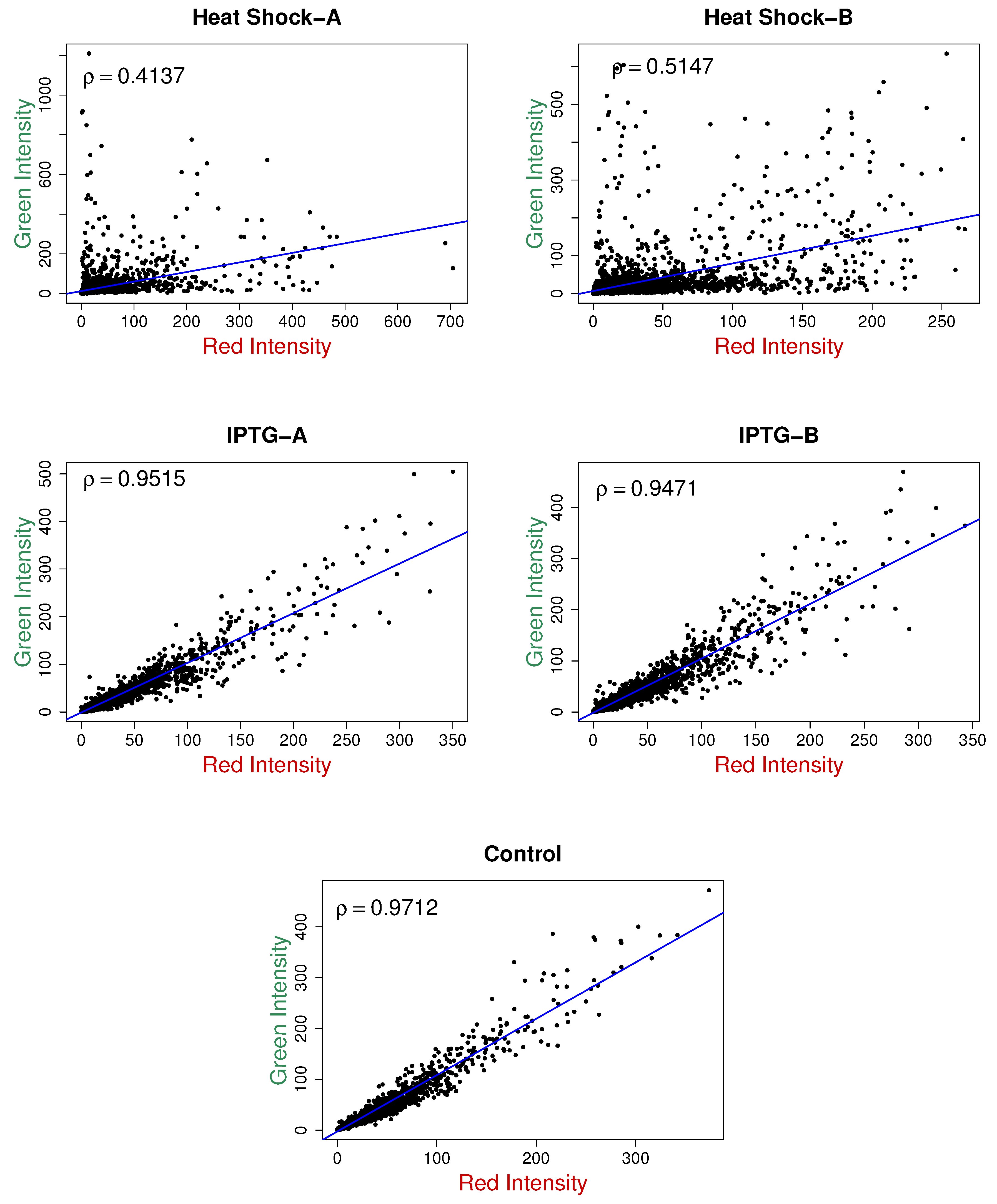
The scatter plots for the red and green intensities for the five samples are shown in Figure 3, along with the sample correlation coefficients. There is a high positive correlation between red and green intensities in all five samples. The positively skewed shape of the density curves suggests the assumption of gamma marginals is reasonable. Thus, following [7], as a parsimonious model, we assume the marginal distributions of the red and green intensities as gamma with standard shape parameters but different scale parameters.

Table 3. Parameter estimates (standard errors) for the E. coli data.

Microarray	$\mathit{\alpha }$	${\mathit{\alpha }}_0$	$\mathit{\nu }$	$\mathit{\gamma }$
Control	0.796	55.245	1529.876	0.9896
	(0.001)	(0.343)	(1.056)	(0.003)
IPTG-A	0.743	40.048	1149.604	0.9838
	(0.001)	(0.127)	(1.181)	(0.021)
IPTG-B	0.643	27.095	899.997	0.9839
	(0.003)	(0.059)	(0.678)	(0.019)
Heat Shock A	1.777	4.644	24.999	0.8116
	(0.039)	(0.094)	(0.056)	(0.013)
Heat Shock B	1.449	4.613	29.999	0.6507
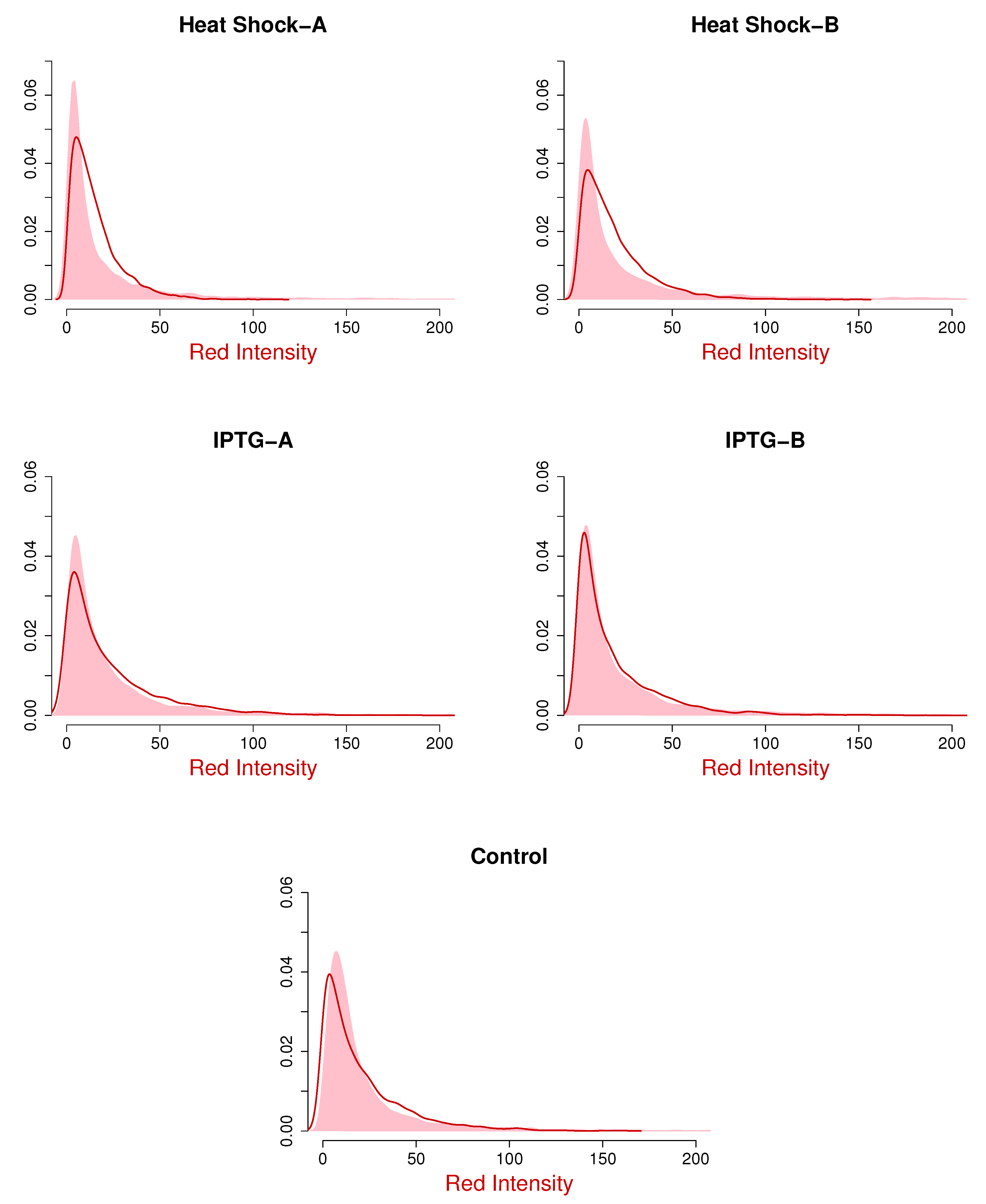
	(0.024)	(0.083)	(0.102)	(0.015)

contains the parameter estimates and their standard errors for the Gaussian copula-based Bayesian models for the five microarray samples. The standard errors are small because the sample sizes are large—more than 4000 in all cases. This suggests that the parameter estimates are pretty accurate.

The empirical density plots, along with the fitted density plots, are shown in Figure 4 and Figure 5 for the red and green intensities, respectively. The solid curves in Figure 4 and Figure 5 are the fitted gamma marginals, and the shaded curves are the empirical plots. Note that the fitted marginals are gamma densities with the estimated parameter values in Table 3. These figures show that the fitted marginals are very good for the IPTG and control samples, but there is some improvement for the heat shock samples, especially the red intensities.

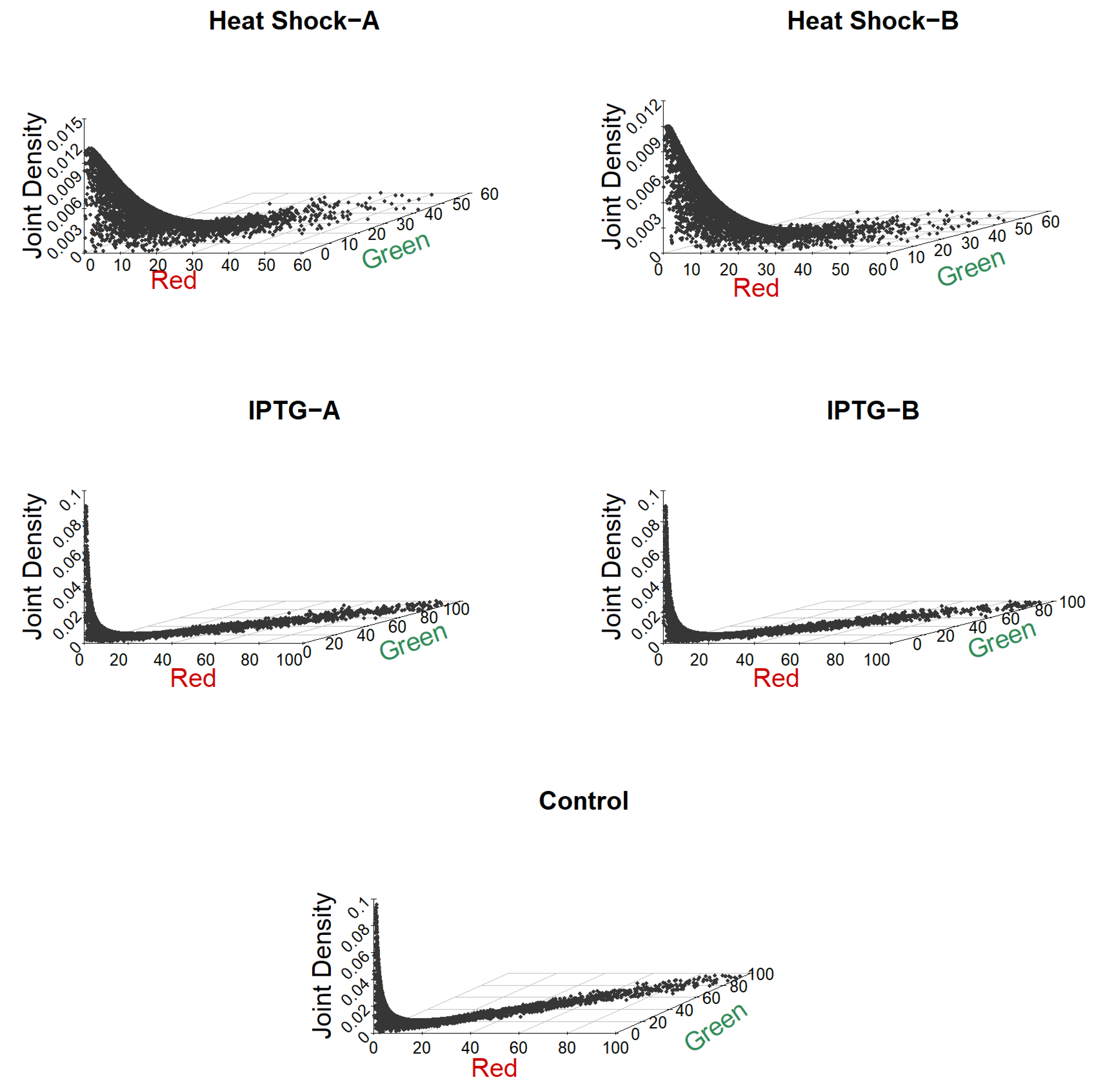
Figure 6 shows the fitted bivariate density plots obtained using the parameter estimates in Table 3. In these plots, the 45° line indicates equal red and green intensities, and the points that fall on this line correspond to genes that are not differentially expressed. We can see that most of the control group’s genes are not differentially expressed using this criteria. For the IPTG samples, a few points lie away from the 45° line, indicating the presence of differentially expressed genes in these samples. Finally, for the two heat shock samples, a large number of points are away from the 45° line, indicating that there is a large number of differentially expressed genes in these samples.

Table 4. True and estimated correlation coefficients.

Microarray	$\mathit{\rho }$	$\widehat{\mathit{\rho }}$
Control	0.9712	0.9748
IPTG-A	0.9515	0.9163
IPTG-B	0.9471	0.9799
Heat Shock A	0.4137	0.4723
Heat Shock B	0.5147	0.3971

displays the observed correlation ($\rho$) and correlation coefficient ($\widehat{\rho }$) calculated from the estimated copula parameter as in Table 3 using Equation (13). Except for Heat Shock B, for all the other four samples, the values of $\rho$ and $\widehat{\rho }$ are very close, indicating that our copula model was fairly successful in quantifying the dependence between the two intensities.

We calculated $\widehat{{\eta }_j}$ using Equation (8), the Bayes estimate $\widehat{{\eta }_j}$ of ${\eta }_j$ which is a measure of differential expression of the jth gene.

Table 5. Top 20 down-regulated genes.

#	Control		IPTG-A		IPTG-B		Heat Shock A		Heat Shock B
	Gene	$\widehat{{\mathit{\eta }}_{\mathit{j}}}$	Gene	$\widehat{{\mathit{\eta }}_{\mathit{j}}}$	Gene	$\widehat{{\mathit{\eta }}_{\mathit{j}}}$	Gene	$\widehat{{\mathit{\eta }}_{\mathit{j}}}$	Gene	$\widehat{{\mathit{\eta }}_{\mathit{j}}}$
	id		id		id		id		id
1	b0233	0.52	b4098	0.29	b4119	0.30	b3686	0.00	b3686	0.04
2	b1325	0.53	b4119	0.29	b4120	0.30	b3687	0.00	b3687	0.05
3	b0558	0.56	b4120	0.45	b4149	0.35	b0014	0.02	b4142	0.05
4	b2843	0.58	b0296	0.53	b0341	0.43	b1306	0.03	b0015	0.05
5	b2129	0.60	b4291	0.54	b4291	0.43	b1967	0.03	b0014	0.05
6	b1319	0.60	b1571	0.54	b1785	0.46	b1304	0.03	b3400	0.06
7	b3818	0.61	b0720	0.56	b1020	0.47	b1380	0.03	b1380	0.06
8	b1075	0.64	b1020	0.58	b0648	0.47	b2614	0.04	b2592	0.07
9	b1924	0.65	b3908	0.59	b0558	0.50	b0399	0.04	b1306	0.08
10	b2742	0.66	b1500	0.60	b2260	0.52	b1305	0.04	b0966	0.08
11	b1447	0.67	b0326	0.60	b0705	0.55	b1307	0.04	b4143	0.08
12	b3341	0.68	b3962	0.60	b0720	0.55	b4143	0.04	b1304	0.08
13	b3751	0.68	b4149	0.61	b3489	0.56	b4140	0.05	b1307	0.08
14	b2756	0.68	b0702	0.62	b0302	0.56	b3400	0.05	b1305	0.08
15	b1166	0.68	b1018	0.63	b3342	0.57	b4142	0.05	b2614	0.09
16	b2051	0.68	b4247	0.63	b1166	0.58	b3401	0.05	b0473	0.09
17	b2541	0.68	b1685	0.64	b0805	0.60	b1321	0.05	b0016	0.09
18	b3340	0.69	b2260	0.65	b1681	0.60	b0473	0.05	b3932	0.09
19	b3966	0.70	b0705	0.65	b2843	0.61	b1829	0.06	b1060	0.10
20	b2628	0.70	b0726	0.66	b3508	0.61	b4171	0.07	b1829	0.10

displays the top twenty down-regulated ($\widehat{{\eta }_j}$ is small) genes, and

Table 6. Top 20 up-regulated genes.

#	Control		IPTG-A		IPTG-B		Heat Shock A		Heat Shock B
	Gene	$\widehat{{\mathit{\eta }}_{\mathit{j}}}$	Gene	$\widehat{{\mathit{\eta }}_{\mathit{j}}}$	Gene	$\widehat{{\mathit{\eta }}_{\mathit{j}}}$	Gene	$\widehat{{\mathit{\eta }}_{\mathit{j}}}$	Gene	$\widehat{{\mathit{\eta }}_{\mathit{j}}}$
	id		id		id		id		id
1	b4325	1.89	b2206	2.32	b1256	2.56	b3556	20.65	b3556	15.68
2	b0657	1.79	b1256	2.30	b2206	2.47	b2094	19.03	b1078	14.71
3	b2740	1.70	b0043	2.22	b0759	2.32	b1076	15.56	b0907	12.44
4	b0542	1.69	b1673	1.97	b4307	2.11	b1077	14.40	b1857	10.89
5	b0679	1.50	b2205	1.95	b1674	2.05	b1075	14.24	b1074	10.28
6	b4314	1.50	b2204	1.95	b2997	2.03	b1857	14.12	b1076	9.91
7	b2418	1.49	b2997	1.94	b2203	2.03	b0754	14.11	b0296	9.87
8	b3616	1.48	b0115	1.90	b2151	2.02	b1074	13.85	b2094	9.51
9	b4243	1.48	b0759	1.89	b0733	2.01	b2926	13.49	b1588	8.81
10	b0185	1.47	b2727	1.89	b0857	2.00	b1073	12.11	b1245	8.22
11	b1084	1.45	b2241	1.83	b2204	1.99	b2935	11.27	b4025	8.18
12	b3834	1.44	b0283	1.81	b2242	1.97	b3544	10.66	b4328	7.97
13	b2860	1.44	b2202	1.80	b2205	1.95	b1078	10.32	b1885	7.89
14	b0729	1.44	b2996	1.80	b2996	1.95	b0907	9.60	b2241	7.17
15	b1083	1.43	b0347	1.78	b2957	1.92	b2416	9.05	b1244	7.12
16	b1064	1.42	b0733	1.78	b2727	1.91	b2092	8.93	b1417	7.03
17	b2283	1.42	b2957	1.78	b2149	1.90	b2286	8.84	b0131	6.70
18	b3147	1.42	b2203	1.76	b2241	1.90	b3357	8.73	b1938	6.63
19	b1674	1.41	b2151	1.75	b0598	1.88	b0893	8.10	b1676	6.57
20	b0698	1.41	b2242	1.74	b0894	1.87	b1244	8.06	b1072	6.53

lists the top twenty up-regulated ($\widehat{{\eta }_j}$ is large) genes for all five samples.

Plots of ordered $\widehat{{\eta }_j}$ values for the five samples are displayed in Figure 7. These plots are S-shaped; the left tails contain the down-regulated genes, whereas the right tails contain the up-regulated genes. In their paper, ref. [16] have listed the genes significantly affected by heat shock and IPTG treatments. According to their findings, the control sample has none of the differentially expressed genes, the IPTG samples have few, and the heat-shock samples have many differentially expressed genes. Therefore, by considering the number of differentially expressed genes and the plots of $\widehat{{\eta }_j}$ of five microarrays, $\widehat{{\eta }_j}=2$ is a good candidate cut-off value to filter up-regulated genes, while $\widehat{{\eta }_j}=0.5$ is for down-regulated genes. The horizontal lines in Figure 7 indicate the possible cut-off values to separate the normal genes from the two extremes.

The total number of differentially expressed genes for each microarray is listed in

Table 7. Total number of differentially expressed genes.

Microarray	# of Genes for Which
	$\widehat{{\mathit{\eta }}_{\mathit{j}}}\mathbf{>}\mathbf{2}$		$\widehat{{\mathit{\eta }}_{\mathit{j}}}\mathbf{<}\mathbf{0}.\mathbf{5}$
	Bivariate	Gaussian	Bivariate	Gaussian
	Gamma	Copula	Gamma	Copula
Control	0	0	0	0
IPTG-A	10	3	3	3
IPTG-B	21	9	7	8
Heat Shock A	553	451	1007	439
Heat Shock B	856	600	590	169

, along with the total number of differentially expressed genes filtered with the bivariate gamma model proposed by [8].

As expected, none of the genes are identified as differentially expressed in the control sample, and very few in IPTG-A and IPTG-B. Many genes were filtered as up- or down-regulated from both the Heat Shock A and Heat Shock B models. The number of genes filtered from the Gaussian copula model is somewhat smaller than that from the bivariate gamma model.

The best model cannot be determined by looking at this total number of genes. Therefore, the log-likelihoods for the two models under each microarray are compared and shown in

Table 8. Log-likelihoods for the competitive models.

Microarray	Bivariate Gamma	Gaussian Copula
Control	−28,824	−28,350
IPTG-A	−28,320	−27,853
IPTG-B	−28,257	−27,885
Heat Shock A	−31,936	−30,419
Heat Shock B	−31,658	−30,282

. The log-likelihood values under our model are higher than those of the bivariate gamma model, which was proposed by [8] for each microarray. Hence, we conclude that the Gaussian copula-based Bayesian model achieves an improvement over the model given in [8]. Further, our method’s filtered differentially expressed genes of heat-shock samples are well matched with the genes listed in [16]. Recall that, in [16], the control sample had no differentially expressed genes, and the IPTG samples had few, consistent with our findings.

9. Discussion

Various methods have been proposed in the literature to identify differentially expressed genes. In this article, we have developed a Gaussian copula-based Bayesian model for detecting differentially expressed genes in cDNA microarray data. The accuracy of the model’s parameter estimates was demonstrated through two simulation studies with three different sample sizes. We further applied our model to five microarray samples from E. coli. Experimentally identified differentially expressed genes in E. coli are documented in [16]. Using Bayes estimates, our model effectively distinguishes between up-regulated and down-regulated genes. Notably, many of the down-regulated genes identified using our model align with those reported in [8], which introduced a bivariate gamma model for the same E. coli data. However, the higher log-likelihood values obtained under our model compared to [8] suggest an improvement over the bivariate Gamma approach. A key advantage of our Guassian-copula model is its flexibility—it can accommodate any marginal distribution for intensities, whereas the bivariate gamma model is restricted to gamma-distributed marginals. Future research will explore the use of other copulas.