Abstract
Coral-reefs are a significant species in marine life, which are affected by multiple diseases due to the stress and variation in heat under the impact of the ocean. The autonomous monitoring and detection of coral health are crucial for researchers to protect it at an early stage. The detection of coral diseases is a difficult task due to the inadequate coral-reef datasets. Therefore, we have developed a coral-reef benchmark dataset and proposed a Multi-scale Attention Feature Fusion Network (MAFFN) as a neck part of the YOLOv5’s network, called “MAFFN_YOLOv5”. The MAFFN_YOLOv5 model outperforms the state-of-the-art object detectors, such as YOLOv5, YOLOX, and YOLOR, by improving the detection accuracy to 8.64%, 3.78%, and 18.05%, respectively, based on the mean average precision (mAP@.5), and 7.8%, 3.72%, and 17.87%, respectively, based on the mAP@.5:.95. Consequently, we have tested a hardware-based deep neural network for the detection of coral-reef health.
1. Introduction
Coral-reefs play a crucial role in natural marine ecosystems; they serve as the main source of nutrient-rich feed, a significant repository of biodiversity, and a safe environment for marine organisms [1,2]. Coral-reefs help to develop the fishing industry by making fish and other species live near or in the habitats of the corals [3]. However, coral-reef ecosystems are vulnerable to climate change and other man-made activities [4]. In the 1980s, researchers found that the sea surface temperature has been increasing every day due to global warming [5]. Further, thermal stress has degraded corals’ color rapidly, which has affected the corals through bleaching effects. Because of these environmental changes, nearly 30% of coral-reefs have suffered, which may increase to 60% by 2030 [6,7,8].
Figure 1a shows a healthy coral-reef in an underwater scenario, whereas the bleached ones lose their tissues due to environmental stresses such as pollution, variation in temperatures, and salinity, as shown in Figure 1b. The microbial assemblage creates a band of diseases, which destroys the coral tissues and generates the bare coral skeleton, as shown in Figure 1c [9]. The White pox disease in coral-reefs appears as a small circle, and the large white patches are due to the degradation of tissues, as shown in Figure 1d [10]. After the disease is spreads, the coral-reefs become destroyed, which is termed dead coral, as shown in Figure 1e. Consequently, the disease overlay in coral-reefs leads to habitat loss for many marine species.
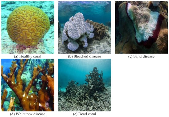
Figure 1.
Coral-reef health conditions.
To detect the disease in corals, an underwater optical imaging system is required to monitor the coral-reef ecosystems frequently. Initially, this coral-reef ecosystem was monitored using photo-quadrats, which were found to be time-consuming to analyze the area covered. Deep learning-based convolutional neural networks have performed automated image processing tasks for coral-reef and fish studies. This technology speeds up and accurately annotates images autonomously and reduces the duration of identifying the coral bleaching within a short span [11,12]. In this paper, a MAFFN_YOLOv5 neural network-based coral-reef health detection system has been proposed. The significant findings of this research are summarized as follows:
- A MAFFN_YOLOv5 neural network is developed to detect the coral-reef health condition.
- A dataset of 3049 high-quality images of coral-reefs comprised of five health conditions such as healthy coral, bleached disease, band disease, white pox disease, and dead coral images were collected and manually annotated.
- Experimental results obtained from the benchmark dataset of the proposed method outperform the other state-of-the-art object detectors such as YOLOv5, YOLOX, and YOLOR in terms of improvements in the detection accuracy based on the mean average precision (mAP@.5 and mAP@.5:.95).
- The proposed method achieves a lightweight model size, which helps to implement the proposed model in the embedded systems in a simple and cost-effective manner.
Section 2 reviews the literature on effective methods related to coral-reef disease classification using Convolutional Neural Networks (CNNs). Section 3 covers the workflow of the MAFFN_YOLOv5 method for detecting coral-reef health. Section 4 describes the tools and measures applied to developing and testing the algorithms. Section 5 details the result and discussion, and Section 6 narrates the conclusion of the research work.
2. Related Work
Ani et al. proposed a CNN-based coral-reef image disease classification research work, but it failed to detect coral disease in images and videos [13]. Marcos et al. developed a Feed-forward back-propagation neural network for classifying coral-reefs into three classes: living coral, dead coral, and sand. [14]. Pican et al. initiated texture-based analysis to classify the seabed [15]. Clement et al. developed automatic monitoring of crown-of-thorns starfish (COTS) on coral images [16]. Johnson-Roberson et al. have tested a real-time segmentation of coral images using Gabor-Wavelet Convolution (GWC) [17]. Mehta et al. performed coral-reef colony classification using texture via support vector machines (SVM) [18]. Pizarro et al. suggested grouping objects of similar features for the hierarchical classification of marine habitat detection [19]. Purser et al. proposed machine learning-based automatic estimation of cold water corals and sponges from extracted images in underwater video frames [20]. Stokes and Deane classified the coral-reef images acquired from the photographic quadrat system [21]. Beijbom et al. constructed the Moorea Labeled Corals (MLC) dataset containing 40,000 annotated coral images [22]. Stough et al. developed a supervised learning-based segmentation of “A. cervicornis” coral images [23]. Shihavuddin et al. designed a supervised learning-based classification of coral-reefs in underwater images and mosaic datasets [24]. Villon et al. analyzed supervised learning-based detection and recognition of fish living in the coral environment [25]. Mahmood et al. attempted the classification of coral-reef images from a pre-trained CNN model-VGGnet [26]. Ani et al. reviewed image classification of coral-reefs in submarine images using Improved Local Derivative Pattern (ILDP) based texture extraction [13,27]. It proposed the Z with Tilted Z Local Binary Pattern (Z+TZLBP) [28] and the texture-based Octa-angled pattern for triangular sub-regions (OPT) [29] for the classification of coral-reef images and videos. Mohammad Hossein Shakoor and Reza Boostani derived a coral-reef image classification system using the local binary pattern [30]. Marre et al. utilized a Deep Neural Networks (DNN) based monitoring system for coralligenous reefs [31]. Raphael et al. initiated a fully-automated deep neural network (DNN) based shallow water corals identification in the Gulf of Eilat area [32]. Zhang et al. designed an improved U-Net model for the segmentation of coral orthoimages [33]. Pavoni et al. developed a semantic segmentation techniques-based annotation toolbox named ‘TagLab’ for quick labelling and analyzed coral-reef orthoimages [34]. Kondraju et al. proposed an atmospheric and water column correction technique to remove the noise for detecting coral-reef condition through remote sensing [35]. Liu et al. monitored the mass coral bleaching effects using the thermal stress from sea surface temperature and high spatial-resolution Sentinel-2B remote sensing imagery systems [36]. Williamson et al. developed a fuzzy logic-based Reef Environmental Stress Exposure Toolbox (RESET) for monitoring environmental stressors on shallow coral-reefs [37]. Meng et al. designed a portable toolkit to monitor the health of coral-reefs and diagnose coral thermal stress using image processing software [38]. Carrillo-García and Kolb introduced an indicator framework for monitoring coral-reef ecosystems [39]. Dugal et al. implemented an eDNA metabarcoding tool for coral-reef monitoring and detection [40]. Lamont et al. approached a theoretical marine policy that combines social, economic, and ecological multi-dimensional strategies for coral-reef restoration [41].
From the literature review, it is observed that most of the researchers attempted coral image classification only. Some researchers have developed a computer vision-based annotation toolbox for coral-reef detection applications. To the best of our knowledge, coral health detection in underwater images and videos is in the budding stage. To address this lacuna, an improved coral-reef health detection method has been proposed in this research with the objective of developing a hardware-based autonomous monitoring system.
3. Proposed Model for the Coral-Reef Health Detection System
3.1. Architecture and Methodology of MAFFN-YOLOv5
The MAFFN-YOLOv5 architecture consists of backbone, neck, and head networks, as shown in Figure 2. The backbone comprises of focus layer, cross-stage partial (CSP) module [42], and Spatial Pyramid Pooling (SPP) layer [43] for extracting the features. The neck consists of Multi-Scale Attention Network with a Feature Fusion network for selecting effective features. The head includes the multi-scale prediction modules for better detection using the weighted-boxes fusion method.
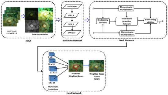
Figure 2.
Architecture of the MAFFN-YOLOv5 model.
3.1.1. Backbone Network
The backbone has three component layers, the focus, CSP, and SPP, as shown in Figure 3, and a slicing operation was employed for the convolution process to avoid information loss. After the slicing, the input image size was converted from 416 × 416 × 3 to 208 × 208 × 12 in the focus layer. Initially, the input image was sliced into four slices, which accommodated 12 output channels, then the concatenation (concat) module was used to fuse the feature maps generated from the sliced images. The convolution (conv) module consists of 40 convolutional layers, which were used to generate multiple feature maps. Then, batch normalization (BN) and leaky ReLU activation functions were performed to get a more stable output with an optimum computation speed. Batch normalization (BN) is used for stability and improves the speed of training the neural networks by regulating the allocation of the input layers during training. It normalized the output features in every layer to a zero-mean level with a standard deviation of one. The ReLU function aids in significantly reducing the learning cycle, while increasing efficiency and speed. In this model, the LeakyReLU function is used as an activation function for solving the gradient loss and dying ReLU issues by applying small positive values to the negative gradient values, which helps to improve the training and classification process. The derivative of the Leaky ReLU activation function is expressed in Equation (1).
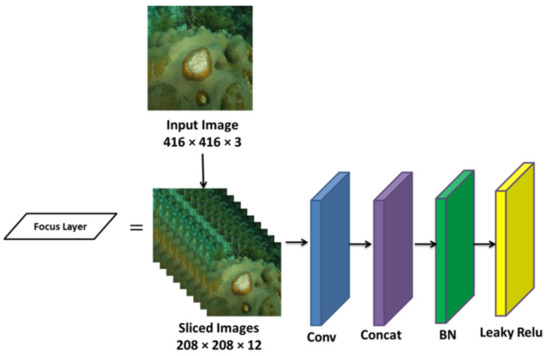
Figure 3.
Architecture of the focus layer.
Figure 4 shows the visualization of the focus layer outputs. From the input image, different features were extracted in each convolutional layer. Initially, the low-level features like the edge and corners of the image features were extracted, then the fine details of the features were obtained.
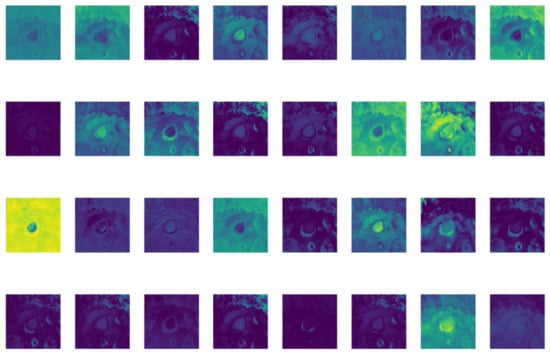
Figure 4.
The visualization of the focus layer output.
The CSP has the advantages of extracting features over propagation, decreasing the parameters in the network, retaining the fine-grained features, and reusing the features for transmitting to further deep layers more effectively. Hence, the CSP was used in the backbone for extracting useful information from the feature, which took the input feature map of the entire image from the base layer, and separated the input into two ways, viz., (i) the dense block for learning the gradient information and (ii) the remaining was directly given to the next block without processing. The YOLOv5s consists of two CSP modules, viz., CSP1_X and CSP3_X, as shown in Figure 5 and Figure 6, respectively. The CSP1_X block consists of CBL block and X*Residual connection units, Conv, Concat, BN, and leaky ReLU layers. Further, the CBL block consists of a convolutional layer (Conv), BN layer, and leaky ReLU layer, as shown in Figure 7. Finally, the CSP3_X block consists of two CBL blocks, Conv, Concat, BN, and leaky ReLU layers.
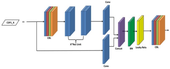
Figure 5.
Architecture of the CSP1_X module.
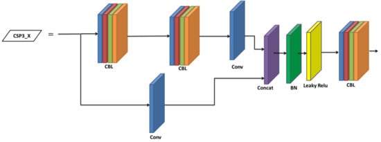
Figure 6.
Architecture of the CSP3_X module.
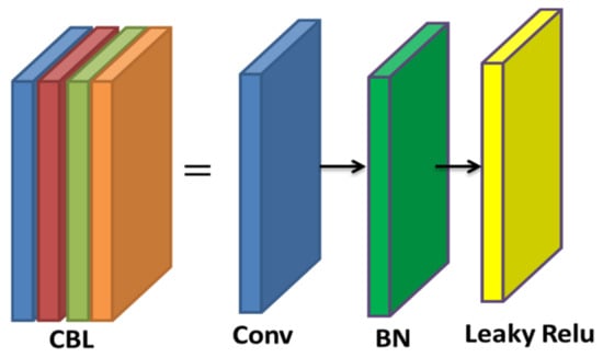
Figure 7.
Architecture of the CBL module.
Figure 8 represents the visualization of the CSP1_X and CSP3_X modules’ output. Here, each convolution layer extracted the significant features in the CSP modules. Therefore, the convolution filters retained the image features at each section of the input image.

Figure 8.
Visualization of the CSP1_X module and CSP3_X module.
The SPP layer was employed at the final block of the backbone for better anchoring and feature maps to solve the fixed-size constraints in the convolutional network. The SPP comprises blocks that come up with two CBL modules, three max-pooling layers, and a Concat block, as shown in Figure 9. In the YOLOv5, the SPP layer’s input feature map size of 416 × 20 × 20 was sub-sampled to 208 × 20 × 20, after transiting the convolution layer kernel size of 1 × 1, which was performed by the CBL module. The input and the resultant feature maps were sub-sampled by three parallel max-pooling layers. Finally, the convolution operation was performed through the CBL module.

Figure 9.
Architecture of the SPP layer module.
The features extracted by the SPP are shown in Figure 10, which exhibits the extracted features as low-visual interpretable envisaged images in the deeper layers.
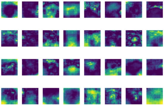
Figure 10.
Visualization of the SPP layer.
3.1.2. Neck Network
The neck is used for better feature extraction from the backbone and reproduces the feature maps from the backbone at various layers. The neck is the primary connection in the object detection network. The MAFFN was used as the neck in the MAFFN-YOLOv5 network [44], since it provides aggregation of local as well as global features from multi-scale and helps to increase the recognition accuracy of the detection network. The pseudo-code of the algorithm is summarized Algorithm 1.
| Algorithm 1: Pseudo code of the algorithm |
| def attention_layer (m, n = 2, out = 64, h_kernel = 1, h_pad = 0, w_kernel = 1, w_pad = 0): def h_pooled (x): for i in range (dense_layers − 1): x = math.ceil (0.5 * (x − 1)) + 1 return int (x) height = calc_pooled_height (100) group = trans_layers + dense_layers for i in range (layers): #conv if i == 0: f.write (layer.generate_conv_layer_str (′attention_layer_conv′ + str (i), ′dense_layer_bn′ + str (dense_layers − 1), ′attention_layer_conv′ + str (i), output * group, h_kernel, w_kernel, h_pad, w_pad, group)) else: f.write (gen_layer.generate_conv_layer_str ( ′attention_layer_conv′ + str (i), ′attention_layer_bn′ + str (i − 1), ′attention_layer_conv′ + str (i), output * group, h_kernel, w_kernel, h_pad, w_pad, group)) f.write (gen_layer.generate_bn_layer_str (′attention_layer_bn′ + str (i), ′attention_layer_conv′ + str (i), ′attention_layer_bn′ + str (i))) f.write (gen_layer.generate_activation_layer_str (′attention_layer_relu′ + str (i), ′attention_layer_bn′ + str(i))) |
The channel attention network was developed by changing the size of the pooling layers to create a lightweight network. Here, the local and global features were aggregated within the attention network, and the point-wise convolution was used as the feature aggregator. For better object detection, the captured contextual information from various network layers was aggregated by semantic and scale-variable features.
In YOLOv5s, the concatenation block was produced as a fixed linear feature fusion of contextual information, and it failed to achieve better detection. Conversely, the MAFFN network is a non-linear network capable of capturing the contextual information on various network layers by aggregating the features irrespective of the different scales. Further, it solves the scale variation problem in channel attention by processing point-wise convolution rather than using various-size kernels.
Figure 11 represents the implementation of the MAFFN_YOLOv5 model by modifying the PANet network in the YOLOv5 model.

Figure 11.
Architecture of the MAFFN module.
The output of an intermediate feature from the backbone network is computed as where represents the width and height of the feature maps and is the local channel context information. Equation (2) represents the point-wise convolution of the feature aggregator.
where A(F) represents the feature aggregator, BN is the batch normalization operator, PWConv1 and PWConv2 are the Point-wise convolution operators, and F is the intermediate feature maps. The convolutional operators’ kernel sizes of PWConv1 and PWConv2 are . The A(F) consists of the same size input feature for preserving and finding the contextual information in the low-level features. Figure 12 portrays the MAFFN module outputs. Here, the convolutional layers abstracted the visual information and changed the image into desired output domain.
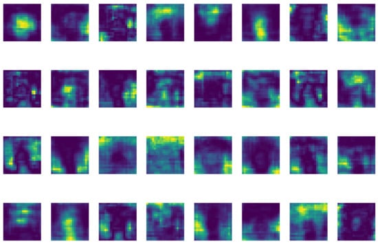
Figure 12.
Visualization of the MAFFN module.
To find the refined features, the local channel context A(F) and global channel context G(F) are modified by the multi-scale attention, as given in Equation (3).
where, is the refined feature and is the multi-scale attention weights. Here, it represents the element-wise multiplication operator and is the broadcasting addition operator.
To utilize the high-level features as well as low-level features, the MAFFN was developed for preserving contextual information from various network layers using semantic and scale-variant features with the objective of enhancing object detection accuracy. Figure 13 represents the architecture of the MAFFN_YOLOv5 Neck network.
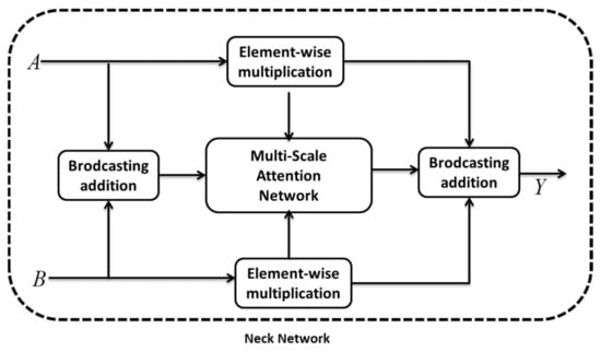
Figure 13.
Architecture of the MAFFN_YOLOv5 Neck network.
Figure 14 illustrates the visualization of the Attentional Feature fusion output. Here, the significant features were extracted well at the stage of the Attentional Feature fusion module.
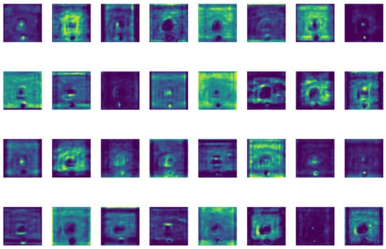
Figure 14.
Visualization of the Attentional Feature fusion module.
The output of Attentional Feature fusion (Y) is derived from the multi-scale channel attention weights and is expressed in Equation (4).
Here, A and B represent low-level semantic and high-level semantic features, respectively. The is the fused feature and represents the initial integration of two features, and . Element-wise integration is used for the initial integration. The fusion weights value should be between 0 and 1, which results in the detection of the weighted-average features.
3.1.3. Weighted-Boxes Fusion-Based Detection
In the object detection task, the backbone and neck networks are not enough to complete the detection and classification of the objects. Thus, the head is designed to categorize the class of the object and locate the object through the feature maps extracted from the neck and backbone [45]. Initially, it generated anchor-boxes on feature maps, which applied the bounding-boxes, analyzed the class probability, and predicted the confidence score [46]. The YOLOv5 is used as a detection head module, which takes significant output features from the MAFFN module as input. The YOLOv5 network utilized feature maps from the neck of the network. YOLOv5 uses the non-maximum suppression (NMS) algorithm [47] for object detection, but it fails in the case of multiple coral-reef disease detection scenarios. Since it detects one detection box as an output, the weighted-boxes fusion (WBF) algorithm [48] was adopted to measure the fusion weights depending on the confidence of the coral-reef disease detection boxes produced from various layers. As a result, the multiple bounding boxes were generated as the output for coral disease detection with high accuracy. WBF algorithm applied a confidence score for all the probability of the bounding boxes to generate the final detection box. If the predictions of bounding boxes for a single image have ‘n’ different models, they generate ‘n’ predictions for the single model from the raw and augmented images. Finally, every predicted bounding box (PBB) from the various models is summed up as a single list L. Then, the list is arranged based on the descending order of the confidence scores (CS). In the list L, every position consists of a set of bounding boxes and forms a cluster. Here, iteration operation is applied to a single image to locate a matching bounding box from the list L. Further, the thresholding level is fixed as 0.5 for better prediction. If the match is located from the list, then the bounding box is applied to the image.
For multiple bounding box predictions, weights are used for the confidence score. The weighted sum of the coordinates of the bounding boxes is assigned to the corresponding boxes. Accordingly, boxes with high confidence scores are used for the multiple box detection than boxes with low confidence scores. The multiple bounding boxes are generated through the confidence score of each coral-reef disease detection and are given in Equations (4) and (5):
In the Equations (5) and (6), , , and are the coordinates of the bounding box. The CS represents the confidence score, n denotes the number of iterations, and X is the number of the bounding-box.
From the possible predicted weighted boxes, the WBF method produces an accurate region of interest when compared with the NMS algorithm. From Figure 15, the black color represents the ground truth bounding box and the red color denotes the final predicted bounding box. The NMS method failed to detect the smaller portions of the diseased area. It is demarcated with a wider bounding box than the actual region of interest, i.e., diseased and non-diseased areas. On the other hand, the WBF method accurately predicted the small and large diseased regions. Thus, the WBF method does not remove any bounding boxes, but it fuses them to demarcate the actual region of interest, very nicely. This method would be a useful feature in the case of multi-class prediction of coral-reef diseases on a single image. Figure 16 represents the visualization output of the weighted boxes fusion module.
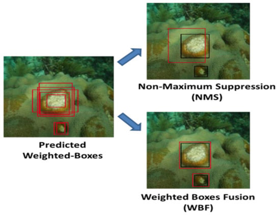
Figure 15.
Comparison results of the NMS algorithm with the WBF method.
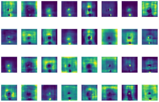
Figure 16.
Visualization of the weighted boxes fusion module.
Here, the significant features were extracted well, and the diseased regions were particularly overlapped with the labeled object, i.e., coral’s white pox diseased region. The final visualization layers illustrate that the proposed model learned the features from the neck part well and exactly localized the diseased region.
4. Tools and Measures
The autonomous monitoring of healthy, disease-affected, and dead coral-reef is necessary to enrich the marine habitat’s productivity. A deep neural network-based system is an effective tool for monitoring this coral-reef health conditions. The deep neural network-based autonomous monitoring tool aids in avoiding human manual errors and helps to monitor the requirements within a short span of time with enhanced accuracy. In the DNN, many neural network architectures have been designed for object detection. We have adopted pre-trained neural networks such as YOLOv5, YOLOR, YOLOX, and MAFFN-YOLOv5 for the object detection model.
4.1. Dataset Collection and Image Augmentation
Due to the inadequate dataset and the difficulty in capturing diverse images and videos from various environments, irrespective of the properties of the images, we have collected and built a benchmark dataset for our research. It comprises coral-reef images collected from Google Images [49], Getty Images [50], Shutter Stock [51], and Coralpedia [52]. The collected images have good variability and complexities like lighting conditions, colored water, occlusion, hazed, angular rotation and orientation, image resolutions, and so on. Then, the collected images were inspected by a specialist to categorize the class and remove the unwanted images. The gathered coral images are categorized manually under five classes: healthy, bleached, white pox, band, and dead corals. Totally, 1000 images were collected and stored as a dataset and those are given as Supplementary Materials. Then, the images were resized from different scales to 416 × 416 images for further processing. Figure 17 shows the building of training dataset after image augmentation. The resized images are augmented from artifacts, such as blurred, mirrored, flipped, hazed, and rotated in various angles, for the training process. Figure 18 shows the workflow of the YOLOv5-MAFFN model-based health detection system.
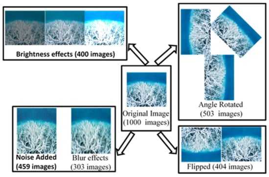
Figure 17.
Training dataset generation through image augmentation process.
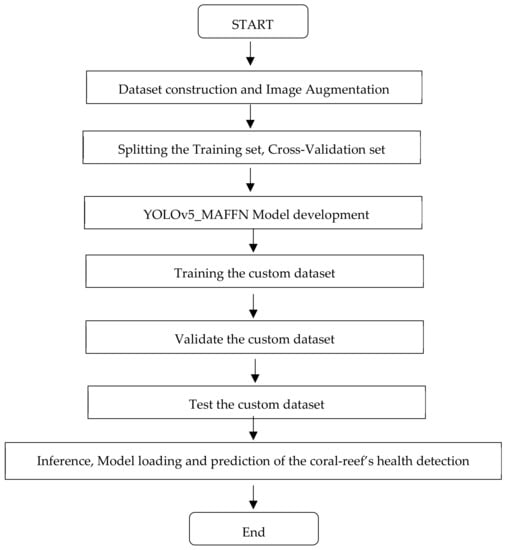
Figure 18.
Flow chart of the YOLOv5-MAFFN model-based health detection system.
4.2. Training and Cross-Validation Details
All the comparative models and the proposed model were implemented on a Workstation system having Intel i5, 4 GB NVIDIA Quadro GPU memory, 16 GB RAM, and 1 TB hard disk memory. To accelerate parallel computing capabilities, the PyTorch framework was framed by CUDA’s (cuDNN) libraries. The configuration of every model’s training detail is described as follows. After the augmentation process, a total of 3069 images were selected and assigned as a coral-reef health detection benchmark dataset. Each class of the dataset was partitioned into 70% images for the training process, 20% images for the validation process, and 10% images for the testing process. From the total number of 3069 images, 70% of images (i.e., 2148) were chosen for the training process, and 20% of images (i.e., 613) were used to validate the prediction accuracy of the trained model. The dataset was separated into a training set and a validation set using the k-fold Cross-Validation method, which helps the model for learning knowledge from the entire collection of data. The processing system was configured with low graphics card memory, i.e., 4 GB, the processing of 720 × 720 resolution images was more complex, and it was replicated as the memory full status after a few epochs. Therefore, the resolution of the input image was resized to 416 × 416, which is sufficient for a quick training process. In the training process, parameters like the number of epochs, the batch size, the learning rate, the momentum factor, and decay rate of weight are user-defined. All the comparative and the proposed models’ epoch number was fixed at 100. The batch size is necessary (to be given) as a hyper-parameter. In this work, genetic algorithms (GA) were applied to obtain optimal hyper-parameters. If the batch size is small, the accuracy of the model becomes low, and if the batch size is too large, it requires a long-computational time. Therefore, to optimize the computational capability, the batch size was given as 16 for all the models. In the MAFFN_YOLOv5, an adaptive moment estimation (Adam) optimizer was used to optimize the learning rate at a low level of 0.0003. Momentum factor and weight decay were fixed at 0.937 and 0.005, respectively. After the training process, the corresponding weight file of the model was saved, and the saved weight file was utilized for testing the model. The model parameters are listed in Table 1.

Table 1.
The default training parameters for the YOLO models.
5. Results and Discussion
5.1. Training Results
During the training process, box_loss, objectness_loss, and classification_loss are the three significant types of losses in the object detection models [53]. Box_loss represents that the prediction is not covering the region of interest in the image. It is a Mean Squared Error (MSE) for bounding box regression loss. Classification_loss denotes the prediction of the region of interest through the bounding box by 1 for the matching class and 0 for other classes, which is called “Cross Entropy”. Objectness_loss is a Binary Cross Entropy loss, which illustrates the wrong bounding box prediction of an object. The loss value is calculated from the variation of the predicted value from the ground truth value. The loss value gets smaller when the prediction value is nearer to the ground truth value, and that model is declared as a better detection performance model.
In the training process, the performance of the proposed model was compared with other object detection models in terms of loss_function and the model weight size. From Figure 19, we observed that the bounding box_loss, classification_loss, and objectness_loss of the training set exhibits a dropping state initially and then stabilized after certain epochs. Among the object detection models, the proposed MAFFN_YOLOv5 model’s loss value was found to be very low and stabilized very well. At the 100 epoch, the box_loss value of the proposed model has attained a value 0.01, but for other models, the box_loss value has taken a range of values from 0.04 to 0.05, as shown in Figure 19a. The lower box_loss value states that the proposed model has better performance than other models and the predicted bounding boxes cover the region of interest accurately. From the objectness_loss, the proposed model’s graph shown in Figure 19b has a value lower than 0.015, but other models have values near 0.025 at the 100th epoch. The lower value of objectness_loss represents that the proposed model has a better prediction of the object through the bounding box than other models. In the case of classification_loss, the proposed model has converged below 0.015, but other models have convergence near 0.025 at the 100th epoch, as shown in Figure 19c. the proposed model has a lower classification_loss value, which implies that the proposed model predicts the region of interest with the perfect classification of the object category than the other models. Thus, the proposed model has performed the classification very well, as is evident from the lower box_loss, objectness_loss, and classification_loss values. Further, the speed of the training process can be accelerated by optimizing the neural network’s architecture.
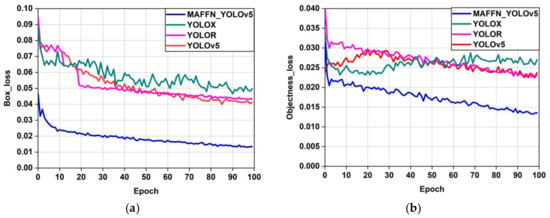
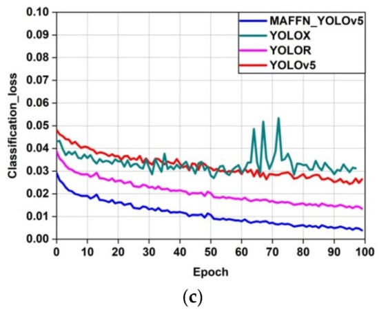
Figure 19.
Comparison of box_loss (a), objectness_loss (b), and classification_loss (c) of the proposed MAFFN_YOLOv5, YOLOR, YOLOX, and YOLOv5.
Table 2 illustrates the training results of the proposed model along with other object detection models. In terms of the model weight size, the MAFFN_YOLOv5 model consists of only 89 MB, i.e., around half (½) of the model weight is reduced compared with the original YOLOv5 model. In contrast, YOLOX and YOLOR models have a higher model weight than the other models. The lesser weight size is preferable to deploy the specific model in hardware devices. Compared with other models, the proposed model has an optimized weight size, which will favor the choice for real-time application. The proposed model took 10.50 h to train the model, whereas the other models consumed more time to complete the training process. Finally, the total number of parameters used in the proposed model is half (½) million times less than the original YOLOv5. Thus, the proposed model ensures low weight and speed among other object detection models.

Table 2.
Performance comparison of training results of the object detection models.
Cross-Validation of the Dataset
The proposed model should be fitted to the training dataset while fitting the model’s hyper-parameters, when objectively evaluated using the validation dataset. The validation datasets are utilized to avoid over-fitting error. It is otherwise called as early stop-regularization of the training process. If the errors increase in the validation dataset, the training process stops and the results in the over-fitting error will be shown in the training dataset. To prove the versatility of the proposed model, mean average precision (mAP@0.5 and mAP@0.5:0.95), Precision (P), Recall (R), and Precision-Recall (P-R) were studied to cross-validate the proposed algorithm. The mean average precision (mAP) is expressed in Equation (7).
where is the number of classes (i.e., health conditions of coral-reefs), N represents the number of Intersection over Union (IoU) threshold, P(t) and R(t) denotes the precision and recall, respectively, and t is the IoU threshold. The mAP@0.5 is the mAP of intersection over union (IOU), which has a fixed threshold of 0.5, and mAP@.5:.95 was calculated by averaging the mAP by varying the threshold level from 0.5 to 0.95. Equations (8) and (9) represent the definition of the Precision and Recall curves, respectively.
Here, TP is the true positive value, and FP and FN are the False-positive and False-negative values, respectively. TP represents the true detection of the disease affected coral-reefs, FP defines the false detection of the disease when there is no disease in the image, and FN represents that the disease is not detected even though the image is a diseased one.
Figure 20a is the IOU threshold at 0.5, in which the MAFFN_YOLOv5 model has a higher value of 0.9 than the other object detection models, which exhibits the performance of the proposed model’s object detection in the training phase. In the case of mAP 0.5:0.95, the threshold varies from 0.5 to 0.95, and the corresponding results of the models are drawn as a graph, as shown in Figure 20b. From the graph, the curve is gradually increased and stabilized after the eight epochs, whereas the other models achieved lesser values than MAFFN_YOLOv5, which denotes that the proposed model achieved a high and stable response for the threshold levels from 0.5 to 0.95 (mAP@0.5:0.95).
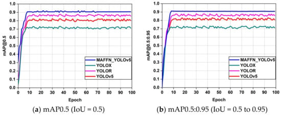
Figure 20.
Performance comparison of the mean Average Precision (mAP) value of MAFFN_YOLOv5, YOLOR, YOLOX, and YOLOv5 models.
In Figure 21a,b, the precision and recall curves gradually increased up to 10 epochs, and afterward, they stabilized. Further, the proposed model reached above 90% level, even though the other models attained lesser values, between 70% to 85%, which predicted that the proposed model detected the object more precisely than the others.
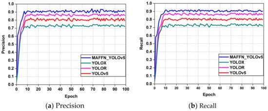
Figure 21.
Comparison of the Precision and Recall plots on the coral-reef dataset.
From the PR curve of the MAFFN_YOLOv5 model shown in Figure 22, it is confirmed that the validation of the proposed model achieves better detection performance, which is inferred from the closer PR curves at the upper-right corner. Further, for the bleached disease corals, the PR value is found to be significantly closer to the right corner, which indicates that the PR value for bleached disease detection attained a high value for the proposed model. Finally, the coral-reef health detection shown in Figure 22 (the black color line) indicates that all the classes have achieved 0.901 (90.1%) PR values for the proposed model. Thus, the proposed model detects the healthy, dead, and all diseased coral-reefs very precisely compared with other models.
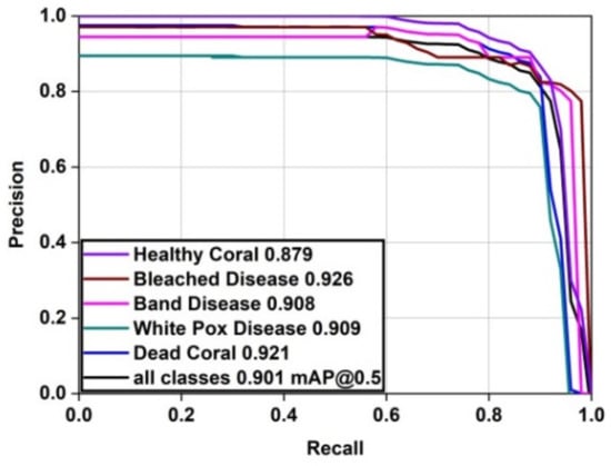
Figure 22.
P-R curves of various health condition classes for the proposed model.
In Table 3, the values of different performance measures were calculated from the benchmark dataset and tabulated to evaluate the accuracy of the proposed model. Compared with other models, the proposed models’ accuracy has significantly improved. In Table 2, the mAP value of the proposed MAFFN_YOLOv5 model achieved the highest values, which were 8.64%, 3.78%, and 18.05% higher than the YOLOv5, YOLOR, and YOLOX models, respectively. By varying the threshold from 0.5 to 0.95, the mAP value of the proposed model is increased by 7.8%, 3.72%, and 17.87% than the YOLOv5, YOLOX, and YOLOR models, respectively. Further, the proposed models’ precision values were 10.73%, 5.41%, and 18.8% higher than the YOLOv5, YOLOX, and YOLOR models, respectively. Moreover, the recall value of the proposed model attained 10.93%, 3.97%, and 17.18% higher values than the YOLOv5, YOLOX, and YOLOR models, respectively. An average detection speed of 9 ms/image is achieved for the proposed model, which is an 11, 7, and 22-fold increase in the speed of the YOLOv5, YOLOR, and YOLOX models, respectively. Consequently, the proposed model achieved the highest mAP@0.5, mAP@0.5:0.95, precision, and recall values, which is highlighted in bold font in Table 2. Thus, the proposed model more accurately detected the coral-reef health condition than the other models. Additionally, the proposed model achieved a very short inference time for a single image, which is a desirable feature for real-time applications.

Table 3.
Quantitative comparison of the proposed and other object detection models.
5.2. Testing the Proposed Model
The models were tested after the training process. From the total number of 3069 images, 10% of images (i.e., 306) were used for the testing process. The confidence threshold value of the object detection model was initially set at 0.5 since a lower threshold value increases the number of false positive bounding boxes and detects the diseases wrongly, whereas a higher threshold value will not detect the disease in the image. Therefore, the selection of the appropriate confidence threshold plays an essential role in the object detection model. To test the detection accuracy of the proposed model, an image was selected randomly from the dataset. The proposed model performed very well in identifying the test image than the other models, which is evident from Figure 23. Here, the coral-reef has no diseases in any area of the entire image, which was detected as a healthy coral-reef (ROI) using the neural networks. The neural network analyzed the input from the pre-trained model and explored the healthy coral-reef with a bounding box based on the accuracy value. The proposed model predicted the bounding box more precisely on the healthy area from the ground truth bounding box of the test image. The ground truth bounding box was generated using manual labeling, where the healthy coral appeared in the entire image. The detection accuracy of 83.9%, 80%, 85%, and 87% was achieved for the YOLOv5, YOLOR, YOLOX, and the proposed MAFFN_YOLOv5, respectively. The proposed models’ accuracy value was increased by 2% than the original YOLOv5 model. Further, there is a 7% and 3.1% increase in the accuracy of the proposed model to the YOLOR and YOLOX models, respectively.
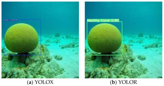
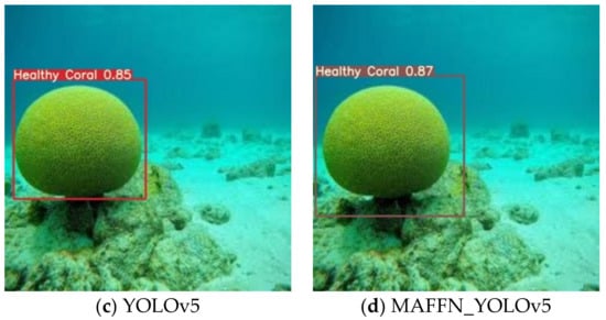
Figure 23.
Healthy coral-reef detection.
Figure 24 shows the detection ability of the models for the coral affected with bleached disease. To demarcate the diseased area, the neural network takes the input from the pre-trained model. The proposed model predicted the bounding box more precisely on the diseased area from the ground truth bounding box of the test image, due to high mAP and IoU. Initially, the ground truth bounding box was generated using manual labeling where the bleached disease affected the image. The accuracy values of 78.5%, 66%, 68%, and 92% were estimated for YOLOX, YOLOR, YOLOv5, and MAFFN_YOLOv5 models, respectively. Compared with the other models, the proposed model achieved 13.5%, 26%, and 24% higher accuracy values than its counterparts.
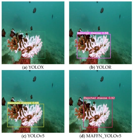
Figure 24.
Bleached disease detection.
Figure 25 shows the results of band disease detection from the benchmark dataset. To detect the band diseased region, the neural network trained the pre-trained model and predicted the results using bounding box and precision values. In Figure 25, the two band diseased coral-reef images were merged as a single image for testing. Here, the upper region of the healthy coral-reef was affected by the band disease. The YOLOX and YOLOR models detected the diseases on both the disease affected images at the accuracy of 88.9% and 82.8%, and 91% and 64%, respectively. In the case of YOLOX model, another bounding box was overlapped in the diseased region and represented the healthy coral with an accuracy value of 32.5%. The YOLOv5 model did not detect the band disease in the upper region of the coral-reef and only detected the lower region of the image at an accuracy of 88%. This is due to some variation in the IoU, and the model does not fit in the ground truth bounding box. However, the proposed model achieved 89% and 90% accuracy values and precisely drew both the diseased regions as a bounding box without any error.
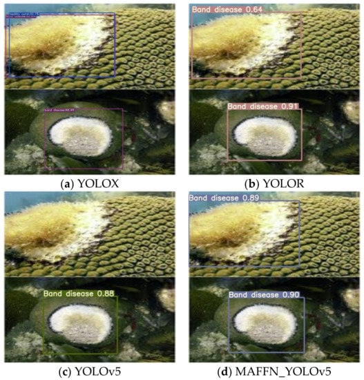
Figure 25.
Band disease detection.
Figure 26 shows an image having two regions affected with white pox disease detected by the models. The pre-trained model has predicted the region of interest, i.e., white pox disease affected region, from the whole test image. The proposed model precisely demarcates more white pox diseased regions by positioning the bounding box at the affected regions. In the case of the YOLOX model, the white pox disease was identified with an accuracy of 59.2%. Still, the positioning of the bounding box occupied a wider area than the actual white pox diseased region, which is due to the variation of the IoU.
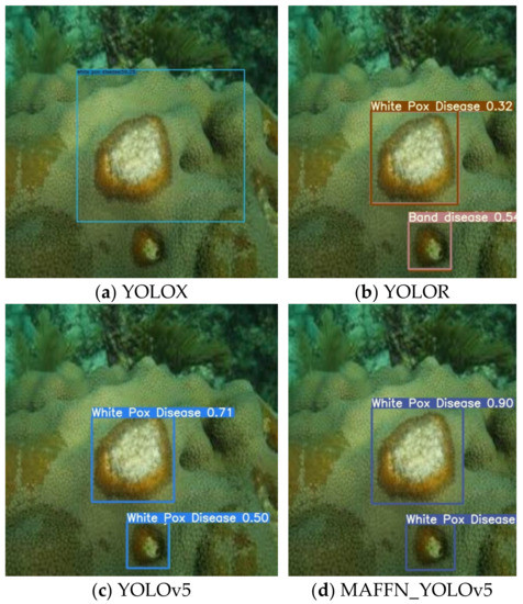
Figure 26.
White pox disease detection.
Further, the YOLOX model did not recognize another white pox diseased region. However, the YOLOR model detected two white pox diseased regions with a low accuracy of 32% and 73%. Conversely, the overlapped bounding box detected the disease as band disease with an accuracy of 54%. Whereas the proposed model has an accuracy of 90% for one of the white pox diseased regions and 89% for another, the YOLOv5 model detected two white pox diseased regions with an accuracy of 71% and 50%. Based on these results, the proposed model achieved 90% and 89% higher accuracy than the other models by precisely drawing the bounding box as per the expected features. Thus, the proposed model is more reliable for detecting white pox disease in coral-reefs.
Figure 27 shows the dead coral and other objects like fish in the test image. To recognize the dead corals, the pre-trained model was applied to the image. Further, predicting the region of interest by demarcating objects and fish from one other was difficult. The proposed model precisely detected the accurate position of the bounding box of the dead coral with an accuracy of 94% and 89%. However, other models predicted the dead corals with an accuracy of 37.2%, 31%, and 62%, respectively. Thus, the proposed model improved detection accuracy by 56.8%, 63%, and 32%, respectively, compared with the other three models. Importantly, the lower regions of the dead coral-reefs were detected promisingly. Thus, the proposed model is more effective for the detection of the dead corals.
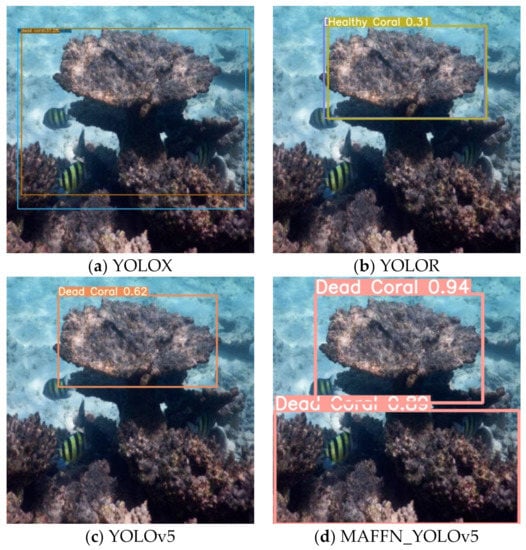
Figure 27.
Dead coral detection.
5.3. Experiment on Multiple Detection and Missing Instances Scenarios
The effectiveness of the proposed method was examined under multiple detections and missing instances to assess its detection efficiency under natural environments, which helps to explore the capability of the proposed method in detecting various disease-affected corals in the given test image. Additionally, missing instances investigated the missing identification of the natural disease-affected area in some test images. Figure 28 shows the multiple health detection of coral-reefs in a single image. In terms of the multiple detection scenarios, the proposed model predicts two types of diseases at a time, i.e., bleached disease with an accuracy of 83% and healthy coral-reefs with an accuracy of 84%, 90%, and 92%. Other object detectors failed to achieve the multiple disease-affected regions in a single test image. The YOLOX model detected one bleached disease and one healthy coral-reef with an accuracy of 81.1% and 37%, respectively, but failed to detect other health conditions of coral-reefs, which were demarcated with a wide bounding box. Whereas the YOLOR model detected two healthy coral regions with an accuracy of 80% and 57% and one bleached disease with an accuracy of 83% but failed to detect the health condition of other coral-reefs. In YOLOv5, bleached disease was represented as dead coral with a single bounding box with an accuracy of 38%. Therefore, the proposed model has solved the various coral-reef diseases missed instance detection problems. The proposed method could effectively extract the significant features for the possible identification of diseases at a time. Other models failed to recognize the detection of small regions of the disease-affected coral-reefs.
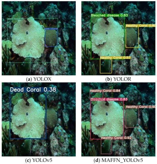
Figure 28.
Multiple and missed detections.
5.4. Noise-Based Experiment
To verify the adaptability of the proposed method, the synthetic noises were added randomly to the input image, despite the noise added already during the image augmentation process of the dataset generation. The noise-affected images were tested in the model, and the results are given in Figure 29. The YOLOX model predicted the bleached disease at 83.1% and healthy disease at 25.9%, whereas the YOLOR and YOLOv5 models predicted the bleached disease at 66% and 88%, respectively. Among them, the proposed model achieved a high prediction accuracy of 92% for the bleached disease even though the images were added with noise.
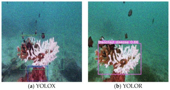
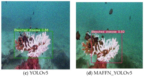
Figure 29.
Results of noise-affected bleach disease detection.
Error Evaluation Performance Metrics
To validate the efficiency of the proposed model for the noisy accrued images, the noise error evaluation performance metrics such as Peak signal-to-noise ratio (PSNR), Mean square error (MSE), Mean Absolute Error (MAE), Mean Average Percentage Error (MAPE) were calculated for the bleached disease detection and the comparative study was performed with other object detection models. The results obtained are illustrated in Table 4. For a good model, the error evaluation measures should have higher PSNR values and lower MSE, MAE, and MAPE values, which predicted higher in the proposed model.

Table 4.
Comparison of Error Evaluation performance metrics calculated for various object detection models with the proposed model.
5.5. Ablation Study
To examine the universality of the proposed model, the ablation study was experimented with in different environments (open agriculture). Here, one of the typical computer vision applications called apple object detection, an emerging application in the agriculture sector, was attempted. With the advent of deep learning, the agriculture industry has seen significant advances in addressing most of its problems and assuring the highest possible product quality. Therefore, accurate detection of the apple in a tree is essential for the autonomous agriculture robotic application. In the open environment, the artifacts such as occlusion, blurring, low-contrast, and so on, are affected the image of the apple, which impediments the prediction accuracy. Figure 30 shows the results of the detection of apple images (five numbers) in the open environment. Among other models, the proposed model has predicted all five apples with accuracy of 94%, 93%, 72%, 58%, 48%, and 38%, whereas the YOLOX and YOLOR models have predicted two apples only. However, YOLOv5 model predicted only three apples, which proved its inability to compete with the prediction accuracy of the proposed model. Thus, the proposed model is more effective in detecting the apple in the open environment.
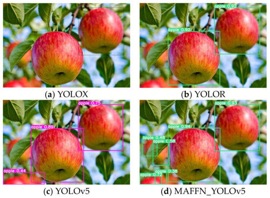
Figure 30.
Results of the ablation study for the apple detection.
5.6. Hardware Implementation
The trained model was deployed on the edge device, called NVIDIA Jetson Xavier NX [54], as shown in Figure 31. It comprises a CPU with 6-core NVIDIA Carmel ARM® v8.2 64-bit processor, GPU with NVIDIA Volta architecture containing 384 CUDA cores and 48 Tensor cores, and requires low power, i.e., 10 W power. It is capable of high-resolution processing data and running multiple neural networks at a time. The NVIDIA Jetson Xavier NX has Jetpack SDK version 4.6.1, which comprises Jetson Linux Driver Package (L4T) with Linux operating system and CUDA accelerated (cuDNN) libraries for computer vision and deep learning with TensorRT for accelerating computers. The CUDA libraries reduce the calculation time to optimize the operations like addition and multiplication in deep neural networks. Pytorch and OpenCV libraries were configured to implement the proposed model on Jetpack SDK. Even though Jetson Xavier NX is a portable device that can use for remote applications, it is not suitable for training the large dataset of deep learning models. Therefore, the training was done on a GPU workstation; thereafter, the best model was deployed on Jetson Xavier NX.
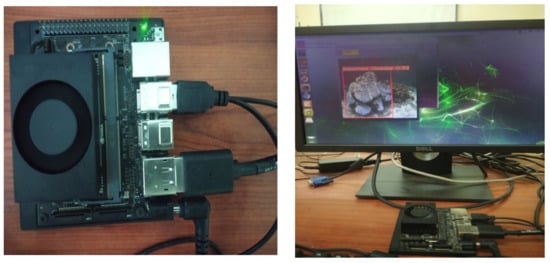
Figure 31.
NVIDIA Jetson Xavier NX board-based coral-reef health detection system.
Video Inference on NVIDIA Jetson Xavier NX Board
To validate the video inference on coral-reef health condition, the input video was taken at 25 frames/sec with a resolution of 1280 × 720. The inference time of the proposed model was estimated as 0.5 ms. Other detection models processed the test image at the speed of 11 ms, 7 ms, and 13 ms for the YOLOX, YOLOR, and YOLOv5, respectively. The results imply that the proposed model satisfied the hardware requirements of real-time coral-reef disease detection. Table 5 illustrates the execution time comparison of the Jetson Xavier NX board-based coral-reef health detection system. Figure 32 shows the implementation of NVIDIA Jetson Xavier NX board-based coral-reef health detection system.

Table 5.
Execution time comparison of the Jetson Xavier NX-based health detection system.
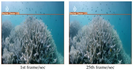
Figure 32.
Snapshot of video inference on NVIDIA Jetson Xavier NX board.
The Jetson Xavier NX board-based health detection system has low power consumption, low memory, and low computation cost with a high inference speed. Figure 32 shows the snapshot of the coral-reef health detection using the proposed model. As a result, the proposed model is most suitable for developing hardware-based real-time coral-reef health detection systems.
6. Conclusions
This research work tries to unravel the possibilities of constructing an autonomous system for detecting coral-reef health conditions using the latest image processing strategies. At the outset, this research proposed a novel convolutional neural network, “MAFFN_YOLOv5”, for detecting the coral health condition with improved accuracy and speed. For testing the algorithm of the models, a high-quality image benchmark dataset of coral-reefs was constructed, which was utilized for training models. In the proposed MAFFN_YOLOv5 models, the multi-scale feature fusion attention network was used to modify the neck part of the YOLOv5, which yields an accuracy of 90.1% (mAP) on the benchmark dataset. As a result, the proposed model is lightweight, which may solve real-time requirements such as high accuracy, speed, and easy implementation. Consequently, the identification of coral-reef health detection using a benchmark dataset is a vital application and will be considered a remarkable contribution to the computer vision research community. Additionally, the proposed method has been implemented in a hardware-based system to study the feasibility of an automated system detecting coral-reef health conditions. Thus, the hardware-based system has detected the coral’s health condition with high accuracy, speed, and low-cost.
Supplementary Materials
The following supporting information, such as dataset, source code and result videos, can be downloaded at the submission portal https://www.mdpi.com/article/10.3390/analytics2010006/s1.
Author Contributions
Conceptualization, S.K.S.R. and N.D.; methodology, S.K.S.R. and N.D.; software, S.K.S.R.; validation, S.K.S.R. and N.D.; formal analysis, S.K.S.R. and N.D.; investigation, S.K.S.R. and N.D.; writing—original draft preparation, S.K.S.R.; writing—review and editing, S.K.S.R. and N.D.; visualization, S.K.S.R.; supervision, S.K.S.R. and N.D.; project administration, S.K.S.R. and N.D. All authors have read and agreed to the published version of the manuscript.
Funding
This research received no external funding.
Institutional Review Board Statement
Not applicable.
Informed Consent Statement
Not applicable.
Data Availability Statement
Given in the Supplementary Materials.
Conflicts of Interest
The authors declare no conflict of interest.
References
- Spalding, D.; Ravilious, C.; Edmund, P. Green World Atlas of Coral Reefs; University of California Press: London, UK, 2001. [Google Scholar] [CrossRef]
- Hoegh-Guldberg, O.N.; Mumby, P.J.; Hooten, A.J.; Steneck, R.S.; Greenfield, P.; Gomez, E.; Harvell, C.D.; Sale, P.F.; Edwards, A.J.; Caldeira, K.; et al. Coral Reefs Under Rapid Climate Change and Ocean Acidification. Science 2007, 318, 1737–1742. [Google Scholar] [CrossRef] [PubMed]
- Mahmood, A.; Bennamoun, M.; An, S.; Sohel, F.; Boussaid, F.; Hovey, R.; Kendrick, G.; Fisher, R.B. Deep Learning for Coral Classification, 1st ed.; Elsevier Inc.: Amsterdam, The Netherlands, 2017. [Google Scholar] [CrossRef]
- Hughes, T.P.; Barnes, M.L.; Bellwood, D.R.; Cinner, J.E.; Cumming, G.S.; Jackson, J.B.C.; Kleypas, J.; van de Leemput, I.A.; Lough, J.M.; Morrison, T.H.; et al. Coral reefs in the Anthropocene. Nature 2017, 546, 82–90. [Google Scholar] [CrossRef] [PubMed]
- Brown, A. No escaping the heat. Nat. Clim. Chang. 2012, 2, 230. [Google Scholar] [CrossRef]
- Hughes, T.P.; Baird, A.H.; Bellwood, D.R.; Card, M.; Connolly, S.R.; Folke, C.; Grosberg, R.; Hoegh-Guldberg, O.; Jackson, J.B.C.; Kleypas, J.; et al. Climate Change, Human Impacts, and the Resilience of Coral Reefs. Science 2003, 301, 929–933. [Google Scholar] [CrossRef] [PubMed]
- Hughes, T.P.; Kerry, J.T.; Álvarez-Noriega, M.; Álvarez-Romero, J.G.; Anderson, K.D.; Baird, A.H.; Babcock, R.C.; Beger, M.; Bellwood, D.R.; Berkelmans, R.; et al. Global warming and recurrent mass bleaching of corals. Nature 2017, 543, 373–377. [Google Scholar] [CrossRef] [PubMed]
- Bourne, D.G.; Garren, M.; Work, T.M.; Rosenberg, E.; Smith, G.W.; Harvell, C.D. Microbial disease and the coral holobiont. Trends Microbiol. 2009, 17, 554–562. [Google Scholar] [CrossRef] [PubMed]
- Rosenberg, E.; Loya, Y. Coral Health and Disease; Springer Science & Business Media: Berlin/Heidelberg, Germany, 2013. [Google Scholar]
- Sharma, D.; Ravindran, C. Diseases and pathogens of marine invertebrate corals in Indian reefs. J. Invertebr. Pathol. 2020, 173, 107373. [Google Scholar] [CrossRef]
- Nunes, J.A.C.C.; Cruz, I.C.S.; Nunes, A.; Pinheiro, H.T. Speeding up coral-reef conservation with AI-aided automated image analysis. Nat. Mach. Intell. 2020, 2, 292. [Google Scholar] [CrossRef]
- Vickers, N.J. Animal Communication: When I’m Calling You, Will You Answer Too? Curr. Biol. 2017, 173, R713–R715. [Google Scholar] [CrossRef]
- Ani Brown Mary, N.; Dharma, D. A novel framework for real-time diseased coral reef image classification. Multimed. Tools Appl. 2019, 78, 11387–11425. [Google Scholar] [CrossRef]
- Marcos, M.S.A.C.; Soriano, M.N.; Saloma, C.A. Classification of coral reef images from underwater video using neural networks. Opt. Express 2005, 13, 8766. [Google Scholar] [CrossRef]
- Pican, N.; Trucco, E.; Ross, M.; Lane, D.M.; Petillot, Y.; Tena Ruiz, I. Texture analysis for seabed classification: Co-occurrence matrices vs. self-organizing maps. In Proceedings of the IEEE Oceanic Engineering Society. OCEANS’98. Conference Proceedings (Cat. No.98CH36259), Nice, France, 28 September–1 October 1998; Volume 1, pp. 424–428. [Google Scholar] [CrossRef]
- Clement, R.; Dunbabin, M.; Wyeth, G. Toward robust image detection of crown-of-thorns starfish for autonomous population monitoring. In Proceedings of the 2005 Australasian Conference on Robotics and Automation, ACRA 2005, Barcelona, Spain, 18–22 April 2005; pp. 1–8. [Google Scholar]
- Johnson-Roberson, M.; Kumar, S.; Pizarro, O.; Willams, S. Stereoscopic imaging for coral segmentation and classification. In Proceedings of the OCEANS 2006, Boston, MA, USA, 18–21 September 2006; pp. 1–6. [Google Scholar] [CrossRef]
- Mehta, A.; Ribeiro, E.; Gilner, J.; Woesik, R. Van Coral Reef Texture Classification. In Proceedings of the VISAPP, Barcelona, Spain, 8–11 March 2007; pp. 302–310. [Google Scholar]
- Pizarro, O.; Rigby, P.; Johnson-Roberson, M.; Williams, S.B.; Colquhoun, J. Towards image-based marine habitat classification. In Proceedings of the OCEANS 2008, Quebec City, QC, Canada, 15–18 September 2008; pp. 1–7. [Google Scholar] [CrossRef]
- Purser, A.; Bergmann, M.; Lundälv, T.; Ontrup, J.; Nattkemper, T. Use of machine-learning algorithms for the automated detection of cold-water coral habitats: A pilot study. Mar. Ecol. Prog. Ser. 2009, 397, 241–251. [Google Scholar] [CrossRef]
- Stokes, M.D.; Deane, G.B. Automated processing of coral reef benthic images. Limnol. Oceanogr. Methods 2009, 7, 157–168. [Google Scholar] [CrossRef]
- Beijbom, O.; Edmunds, P.J.; Kline, D.I.; Mitchell, B.G.; Kriegman, D. Automated annotation of coral reef survey images. In Proceedings of the 2012 IEEE Conference on Computer Vision and Pattern Recognition, Providence, RI, USA, 16–21 June 2012; pp. 1170–1177. [Google Scholar] [CrossRef]
- Stough, J.; Greer, L.; Matt, B. Texture and Color Distribution-Based Classification for Live Coral Detection. In Proceedings of the 12th International Coral Reef Symposium, Douglas, Australia, 9–13 July 2012; pp. 9–13. Available online: http://cs.wlu.edu/~stough/research/coral/ICRS12/Stough_ICRS12_7.pdf (accessed on 5 July 2022).
- Shihavuddin, A.S.M.; Gracias, N.; Garcia, R.; Gleason, A.; Gintert, B. Image-Based Coral Reef Classification and Thematic Mapping. Remote Sens. 2013, 5, 1809–1841. [Google Scholar] [CrossRef]
- Villon, S.; Chaumont, M.; Subsol, G.; Villéger, S.; Claverie, T.; Mouillot, D. Coral Reef Fish Detection and Recognition in Underwater Videos by Supervised Machine Learning: Comparison Between Deep Learning and HOG+SVM Methods. In Proceedings of the Advanced Concepts for Intelligent Vision Systems, Lecce, Italy, 24–27 October 2016; Volume 10016, pp. 160–171. [Google Scholar] [CrossRef]
- Mahmood, A.; Bennamoun, M.; An, S.; Sohel, F.; Boussaid, F.; Hovey, R.; Kendrick, G.; Fisher, R.B. Automatic annotation of coral reefs using deep learning. In Proceedings of the OCEANS 2016 MTS/IEEE Monterey, Monterey, CA, USA, 19–23 September 2016; pp. 1–5. [Google Scholar] [CrossRef]
- Ani Brown Mary, N.; Dharma, D. Coral reef image classification employing Improved LDP for feature extraction. J. Vis. Commun. Image Represent. 2017, 49, 225–242. [Google Scholar] [CrossRef]
- Ani Brown Mary, N.; Dejey, D. Classification of Coral-reef Submarine Images and Videos Using a Novel Z with Tilted Z Local Binary Pattern (Z⊕TZLBP). Wirel. Pers. Commun. 2018, 98, 2427–2459. [Google Scholar] [CrossRef]
- Ani Brown Mary, N.; Dejey, D. Coral-reef image/video classification employing novel octa-angled pattern for triangular sub region and pulse coupled convolutional neural network (PCCNN). Multimed. Tools Appl. 2018, 77, 31545–31579. [Google Scholar] [CrossRef]
- Shakoor, M.H.; Boostani, R. A novel advanced local binary pattern for image-based coral reef classification. Multimed. Tools Appl. 2018, 77, 2561–2591. [Google Scholar] [CrossRef]
- Marre, G.; De Almeida Braga, C.; Ienco, D.; Luque, S.; Holon, F.; Deter, J. Deep convolutional neural networks to monitor coralligenous reefs: Operationalizing biodiversity and ecological assessment. Ecol. Inform. 2020, 59, 101110. [Google Scholar] [CrossRef]
- Raphael, A.; Dubinsky, Z.; Iluz, D.; Benichou, J.I.C.; Netanyahu, N.S. Deep neural network recognition of shallow water corals in the Gulf of Eilat (Aqaba). Sci. Rep. 2020, 10, 12959. [Google Scholar] [CrossRef]
- Zhang, H.; Gruen, A.; Li, M. Deep learning for semantic segmentation of coral images in underwater photogrammetry, ISPRS Annals of the Photogrammetry. Remote Sens. Spat. Inf. Sci. 2022, V-2-2022, 343–350. [Google Scholar] [CrossRef]
- Pavoni, G.; Corsini, M.; Ponchio, F.; Muntoni, A.; Edwards, C.; Pedersen, N.; Cignoni, P.; Sandin, S. Taglab: Ai-assisted annotation for the fast and accurate semantic segmentation of coral reef orthoimages. J. Field Robot. 2021, 39, 246–262. [Google Scholar] [CrossRef]
- Kondraju, T.T.; Mandla, V.R.; Chokkavarapu, N.; Peddinti, V.S. A comparative study of atmospheric and water column correction using various algorithms on landsat imagery to identify coral reefs. Reg. Stud. Mar. Sci. 2022, 49, 102082. [Google Scholar] [CrossRef]
- Liu, B.; Guan, L.; Chen, H. Detecting 2020 coral bleaching event in the Northwest Hainan Island using CORALTEMP SST and sentinel-2b MSI imagery. Remote Sens. 2021, 13, 4948. [Google Scholar] [CrossRef]
- Williamson, M.J.; Tebbs, E.J.; Dawson, T.P.; Thompson, H.J.; Head, C.E.; Jacoby, D.M. Monitoring shallow coral reef exposure to environmental stressors using satellite Earth observation: The Reef Environmental Stress Exposure Toolbox (RESET). Remote Sens. Ecol. Conserv. 2022, 8, 855–874. [Google Scholar] [CrossRef]
- Meng, Z.; Williams, A.; Liau, P.; Stephens, T.G.; Drury, C.; Chiles, E.N.; Bhattacharya, D.; Javanmard, M.; Su, X. Development of a portable toolkit to diagnose Coral thermal stress. Sci. Rep. 2022, 12, 14398. [Google Scholar] [CrossRef]
- Carrillo-García, D.M.; Kolb, M. Indicator framework for monitoring eco-system integrity of coral reefs in the western Caribbean. Ocean. Sci. J. 2022, 57, 1–24. [Google Scholar] [CrossRef]
- Dugal, L.; Thomas, L.; Wilkinson, S.P.; Richards, Z.T.; Alexander, J.B.; Adam, A.A.S.; Kennington, W.J.; Jarman, S.; Ryan, N.M.; Bunce, M.; et al. Coral monitoring in northwest Australia with environmental DNA metabarcoding using a curated reference database for optimized detection. Environ. DNA 2021, 4, 63–76. [Google Scholar] [CrossRef]
- Lamont, T.A.C.; Razak, T.B.; Djohani, R.; Janetski, N.; Rapi, S.; Mars, F.; Smith, D.J. Multi-dimensional approaches to scaling up coral reef restoration. Mar. Policy 2022, 143, 105199. [Google Scholar] [CrossRef]
- Wang, C.-Y.; Mark Liao, H.-Y.; Wu, Y.-H.; Chen, P.-Y.; Hsieh, J.-W.; Yeh, I.-H. CSPNet: A New Backbone that can Enhance Learning Capability of CNN. In Proceedings of the 2020 IEEE/CVF Conference on Computer Vision and Pattern Recognition Workshops (CVPRW), Virtual Conference, 14–19 June 2020; Volume 2020, pp. 1571–1580. [Google Scholar]
- He, K.; Zhang, X.; Ren, S.; Sun, J. Spatial Pyramid Pooling in Deep Convolutional Networks for Visual Recognition. In Proceedings of the Computer Vision—ECCV 2014, Zurich, Switzerland, 6–12 September 2014; Volume 8691, pp. 346–361. [Google Scholar] [CrossRef]
- Dai, Y.; Gieseke, F.; Oehmcke, S.; Wu, Y.; Barnard, K. Attentional Feature Fusion. In Proceedings of the 2021 IEEE Winter Conference on Applications of Computer Vision (WACV), Waikoloa, HI, USA, 3–8 January 2021; pp. 3559–3568. [Google Scholar] [CrossRef]
- Zhu, X.; Lyu, S.; Wang, X.; Zhao, Q. TPH-YOLOv5: Improved YOLOv5 Based on Transformer Prediction Head for Object Detection on Drone-captured Scenarios. In Proceedings of the 2021 IEEE/CVF International Conference on Computer Vision Workshops (ICCVW), Montreal, BC, Canada, 11–17 October 2021; Volume 2021, pp. 2778–2788. [Google Scholar] [CrossRef]
- Wan, J.; Chen, B.; Yu, Y. Polyp Detection from Colorectum Images by Using Attentive YOLOv5. Diagnostics 2021, 11, 2264. [Google Scholar] [CrossRef]
- Hosang, J.; Benenson, R.; Schiele, B. Learning Non-maximum Suppression. In Proceedings of the 2017 IEEE Conference on Computer Vision and Pattern Recognition (CVPR), Honolulu, HI, USA, 21–26 July 2017; Volume 2017, pp. 6469–6477. [Google Scholar] [CrossRef]
- Solovyev, R.; Wang, W.; Gabruseva, T. Weighted boxes fusion: Ensembling boxes from different object detection models. Image Vis. Comput. 2021, 107, 104117. [Google Scholar] [CrossRef]
- [Dataset] Google Images, (n.d.). Available online: https://images.google.com/ (accessed on 5 May 2022).
- [Dataset] Gettyimages, (n.d.). Available online: https://www.gettyimages.in/ (accessed on 5 May 2022).
- [Dataset] Shutter Stock, (n.d.) 348. Available online: https://www.shutterstock.com/ (accessed on 5 May 2022).
- Mees, J.M.; Costello, M.J.; Hernandez, F.; Vandepitte, L.; Gofas, S.; Hoeksema, B.W.; Klautau, M.; Kroh, A.; Poore, G.C.B.; Read, G.; et al. World Register of Marine Species. 2013. Available online: http://www.marinespecies.org (accessed on 5 May 2022).
- Li, S.; Li, Y.; Li, Y.; Li, M.; Xu, X. YOLO-FIRI: Improved YOLOv5 for Infrared Image Object Detection. IEEE Access 2021, 9, 141861–141875. [Google Scholar] [CrossRef]
- The Jetson Developer Kit User Guide. 2021. Available online: https://files.seeedstudio.com/products/102110427/Jetson_Xavier_NX_Developer_Kit_User_Guide.pdf (accessed on 5 May 2022).
Disclaimer/Publisher’s Note: The statements, opinions and data contained in all publications are solely those of the individual author(s) and contributor(s) and not of MDPI and/or the editor(s). MDPI and/or the editor(s) disclaim responsibility for any injury to people or property resulting from any ideas, methods, instructions or products referred to in the content. |
© 2023 by the authors. Licensee MDPI, Basel, Switzerland. This article is an open access article distributed under the terms and conditions of the Creative Commons Attribution (CC BY) license (https://creativecommons.org/licenses/by/4.0/).