Article

Graph Algebras and Derived Graph Operations

Department of Informatics, University of Bergen, 5020 Bergen, Norway
*
Author to whom correspondence should be addressed.
Logics 2023, 1(4), 182-239; https://doi.org/10.3390/logics1040010
Submission received: 12 May 2023 / Revised: 28 August 2023 / Accepted: 11 September 2023 / Published: 17 October 2023
(This article belongs to the Special Issue Combining Logics and Theories)

Abstract

:
We revise our former definition of graph operations and correspondingly adapt the construction of graph term algebras. As a first contribution to a prospective research field, Universal Graph Algebra, we generalize some basic concepts and results from algebras to graph algebras. To tackle this generalization task, we revise and reformulate traditional set-theoretic definitions, constructions and proofs in Universal Algebra by means of more category-theoretic concepts and constructions. In particular, we generalize the concept of generated subalgebra and prove that all monomorphic homomorphisms between graph algebras are regular. Derived graph operations are the other main topic. After an in-depth analysis of terms as representations of derived operations in traditional algebras, we identify three basic mechanisms to construct new graph operations out of given ones: parallel composition, instantiation, and sequential composition. As a counterpart of terms, we introduce graph operation expressions with a structure as close as possible to the structure of terms. We show that the three mechanisms allow us to construct, for any graph operation expression, a corresponding derived graph operation in any graph algebra.

1. Introduction

The paper is a relatively independent part of a broader long-term project to develop a proper foundation of diagrammatic specification formalisms and diagrammatic logics. The project is centered around and extends the concept of generalized sketches. We use the term “diagrammatic” as a synonym for “graph-based” in a very broad sense including arbitrary presheaf topoi.
One of the objectives of our project is to elevate traditional first-order logic to a wide range of arbitrary categories. In [1], we only addressed predicates and showed how to define corresponding first-order logics of statements in context without operations in arbitrary categories. The present paper is also meant to be a first step towards an abstract notion of an operation allowing us to define fully fledged first-order logics of statements in context, at least, in arbitrary topoi.
Generalized sketches have been developed in the 1990s independently by Michael Makkai, motivated by his work on an abstract formulation of completeness theorems in logic [2], and a group in Latvia around Zinovy Diskin, motivated by their work on data bases and data modeling [3,4,5]. Our concept of graph operation has its origins in the concept of sketch operation. Sketch operations do not appear in the work of Makkai, but they have been an integral part of Diskin’s pioneering work from the very beginning.
Graph operations (and their prospective generalizations) are vital in software engineering. Moreover, they provide a conceptual tool with many potential and useful applications in mathematics, logic, and computer science.
Software models are often diagrammatic structures. To keep software models comprehensible for humans, we should, however, avoid overloading them with auxiliary items and redundant information. Nonetheless, to formulate and integrate relevant constraints in software models, it is necessary to refer to items that are not present in a model but that can be derived, like the composition of references, for example. Graph operations are an appropriate tool to refer to and reason about those derivable items in diagrammatic artifacts.
Graph operations are also vital for the definition of query languages for diagrammatic data models, for example. The crucial idea is to formalize queries as derived graph operations built up from basic operations like the operations of Codd’s relational algebra, for example. The potential to formalize query languages for diagrammatic data models was one of Diskin’s main motivations to introduce sketch operations [4].
An example par excellence for the conceptual potential of graph operations in mathematics are categories. Categories can be described as graphs plus an identity and a composition operation. It is not common yet, but quite natural, to consider these operations as graph operations. The identity operation introduces, for each vertex in a graph, a loop, while the composition operation generates, for any two successive edges in a graph, a corresponding composite edge. Even statements like “we assume a category with chosen pullbacks”, for example, can be adequately made precise by means of corresponding graph operations. Ref. [6] seems to be the first paper outlining the potential of graph operations in category theory. Since categories are nowadays widely used in computer science, logic, mathematics, and physics, we will use them as our running example.
In traditional string-based formalisms and logics, terms are the standard tool used to represent and reason about “derivable data”. At the same time, terms give us an adequate tool at hand to represent derived operations, i.e., operations that can be built up from the basic operations in an algebra. Therefore, we generalized in [7] the construction of terms from traditional algebras to graph algebras. The construction of graph term algebras and their characterization as a free construction is the main result in [7]. Unfortunately, our expectation that graph terms would give us a universal and appropriate concept of derived graph operations and substitutions at hand was naive. We realized that the strong interconnection between the “representation of data” and the “representation of derived operations” breaks down in the case of graph operations.
After Section 2, where we list some basic notations, concepts, conventions, and results, the paper presents a further development of the theory of graph operations and graph algebras in two directions—model theory (including term algebras) and derived graph operations.
Model theory: 
In [7], we coined the concept of graph algebra, introduced graph terms, and showed that graph term algebras are free graph algebras. There was, however, no model theory in the sense of traditional Universal Algebra. As a kind of “proof of concept”, we therefore generalize some basic model-theoretic concepts and results from traditional algebras to graph algebras. We concentrate on the concept of “generated subalgebra” and the related problem of characterizing monomorphic and epimorphic homomorphisms.
To tackle this task, we make a substantial effort in Section 3 to revise and reformulate traditional set-theoretic definitions, constructions and proofs in Universal Algebra by means of more category-theoretic concepts and constructions. Relying on this reformulation, we can in Section 4 smoothly transfer concepts, definitions and results from traditional algebras to graph algebras. In particular, we prove that all monomorphic homomorphisms between graph algebras are regular.
In [7], we adapted the original idea of sketch operations [4] and defined the arity of a graph operation as a single graph inclusion. This definition does not allow us, however, to consider projections as legal graph operations. To be closer to the traditional concept of operation in Universal Algebra, and to be able to define an appropriate concept of a derived graph operation, we therefore declare in this paper the arity of a graph operation as a span of graph inclusions. In Section 4.2, we clarify the relation between both versions and discuss to what extent they are equivalent.
To prove that all monomorphic homomorphisms between graph algebras are regular, we also introduce partial graph algebras in Section 4.4. We define a so-called term completion procedure transforming partial graph algebras into total graph algebras. This procedure provides for each signature a free functor from the corresponding category of partial graph algebras to the corresponding category of graph algebras. The construction of graph term algebras turns out to be just a special case of this new procedure.
Derived graph 
operations: To understand why the strong interconnection between “representation of data” and “representation of derived operations” breaks down in the case of graph operations and to find out how to define derived graph operations in an appropriate way, we include in the paper a more in-depth analysis of the concept term and discuss substitution calculi in general in Section 3.4.
In Section 3.7, we recall the construction of syntactic Lawvere theories as it is described in [8], for example. In Section 5.1, we discuss finite product categories and elucidate that terms can be characterized as normal forms for finite product expressions; thus, Lawvere’s original slogan “composition is substitution” can be turned into the slogan “substitution is symbolic composition plus normalization”.
Reviewing the relationship between finite products and tensor products, we identify copying in Section 5.2 as the cause of the problem. We argue that, in the case of graph operations, “copying of data”, as a computation of its own, has to be replaced by the “soldering” of input and (!) output ports of computations.
In such a way, we end up in Section 5.3 with three mechanisms to construct new graph operations out of given ones: parallel composition, instantiation (“soldering” of input and output ports), and sequential composition.
Finally, we introduce in Section 5.4 graph operation expressions with a structure as close as possible to the structure of terms. We define their semantics, i.e., the derived graph operations we have been looking for, by means of the three mechanisms of parallel composition, instantiation and sequential composition.
We complete the paper with some remarks concerning Operations in Topoi in Section 6, a discussion of Related Work in Section 7 and concluding remarks in Section 8.

2. Notations and Preliminaries

C O b j denotes the collection of objects of a category C and C M o r as the collection of morphisms of C , respectively. C ( A , B ) is the collection of all morphisms from object A to object B in C . If the category C is clear from the context, we will often use the more compact notation B A instead of C ( A , B ) . We use the diagrammatic notation f ; g : A C for the composition of morphisms f : A B and g : B C in C . C D states that category C is a subcategory of category D . A category C is small if the collection C M o r , and thus also the collection C O b j , is a set. Cat is the category of all small categories. A category C is locally small if C ( A , B ) is a set for all objects A and B in C . Set denotes the category of all sets and all (total) maps. Cat and Set are not small but locally small.
A (directed multi) graph  G = ( G V , G E , s c G , t g G ) is given by a collection G V of vertices, a collection G E of edges and maps s c G : G E G V , t g G : G E G V assigning to each edge its source and target vertex, respectively [9]. 0 = ( , , i d , i d ) is the empty graph. A graph G is small if G V and G E are sets. A graph homomorphism  φ : G H between two graphs G = ( G V , G E , s c G , t g G ) and H = ( H V , H E , s c H , t g H ) is a pair ( φ V , φ E ) of maps φ V : G V H V , φ E : G E H E such that the following diagrams commute.
Logics 01 00010 i001 The identity graph homomorphism  i d G on a graph G is the pair ( i d G V , i d G E ) of identity maps and composition of graph homomorphisms φ : G H and ψ : H K is performed componentwise, i.e., φ ; ψ : = ( φ V ; ψ V , φ E ; ψ E ) . Graph is the category of all small graphs and all graph homomorphisms between them. The empty graph is the initial object in Graph . For convenience and uniformity, we will often consider a set A as a graph without edges.
The category comprising finite and small graphs as well as the underlying graphs of categories like Cat , Set , and Graph , for example, is denoted by GRAPH , while SET is the category containing all the corresponding collections of vertices and edges, respectively. Correspondingly, we denote the category with all small categories and categories like Cat , Set , and Graph as objects by CAT .
g r ( C ) denotes the underlying graph of a category C , i.e., we have gr ( C ) V : = C O b j and gr ( C ) E : = C M o r . Note that a functor F : C D is just a graph homomorphism F : g r ( C ) g r ( D ) also preserving identities and composition. In other words, the assignments C g r ( C ) , ( F : C D ) ( F : g r ( C ) g r ( D ) ) define a faithful forgetful functor Gr : Cat Graph . It is well known that there is a functor Pth : Graph Cat left-adjoint to Gr assigning to any graph G the corresponding path category  P ( G ) .
In practical applications, it is often more convenient to work with interpretation categories instead of functor categories. An interpretation of a graph G in a category C , denoted by φ : G C , is a graph homomorphism φ from G to g r ( C ) . A natural transformation μ : φ ψ between two interpretations φ : G C and ψ : G C is a family μ v : φ V ( v ) ψ V ( v ) , v G V of morphism in C such that φ E ( f ) ; μ u = μ v ; ψ E ( f ) for all edges f : v u in G . All interpretations of G in C and all natural transformations between them constitute the interpretation category  [ G C ] with composition as the vertical composition of natural transformations. (In [10], interpretations φ : G C are called “models of G in C ” and the notation Mod ( G , C ) is used instead of [ G C ] . For our purposes, the more neutral and general term “interpretation” is more convenient). For any categories C , D the assignments ( F : C D ) ( F : g r ( C ) g r ( D ) ) define a full embedding of the traditional functor category  [ C D ] into the interpretation category [ g r ( C ) D ] .
Obviously, the category Graph is, by definition, isomorphic to the interpretation category [ MG Set ] with MG as the graph E         t g         s c V . On the other hand, the adjunction Pth Gr ensures that for any small graph G the interpretation category [ G C ] is isomorphic to the functor category [ P ( G ) C ] and thus a presheaf topos.
For any set I and any set A the set A I = { a : I A } of all maps from I into A is a categorical product in Set with the family ( π i : A I A i I ) of projections defined by π i ( a ) : = a ( i ) for all a A I . If I is finite with n elements (indices), A I is therefore isomorphic to the n-ary Cartesian product A n of A. If we equip a finite set I n = { i 1 , i 2 , , i n } with a fixed total order i 1 < i 2 < < i n , we can reuse the traditional tuple notation for elements in the Cartesian product A n to also represent the elements in A I n : A map a : I n A is represented by the tuple ( a ( i 1 ) , a ( i 2 ) , , a ( i n ) ) . In this paper, we will often describe a map a : I n A by simply declaring a = ( a 1 , a 2 , , a n ) , i.e., a ( i j ) = a j for all 1 j n . If n = 0 , we have I 0 = , and we will consequently represent the only map a : I 0 A by the empty tuple  ( ) . For any finite set A we denote its cardinality by | A | .
For any inclusion A B of sets, we denote by ι A , B : A B the corresponding inclusion map with ι A , B ( a ) = a for all a A . A graph G is a subgraph of a graph H , G H in symbols, if G V H V , G E H E and the inclusion maps ι G V , H V : G V H V and ι G E , H E : G E H E establish a graph homomorphism ι G , H = ( ι G V , H V , ι G E , H E ) : G H . ι G , H is also called an inclusion graph homomorphism or graph inclusion, for short.
A partial map  f : A B is given by a domain of definition  d o m ( f ) A and a total map from d o m ( f ) into B. The composition f ; g : A C of two partial maps f : A B and g : B C is defined by
  • d o m ( f ; g ) : = { x A x d o m ( f ) , f ( x ) d o m ( g ) } and
  • f ; g ( a ) : = g ( f ( a ) ) for all a d o m ( f ; g ) .
  • We consider any (total) map f : A B as a partial map f : A B with d o m ( f ) = A .

3. Algebras and Term Algebras

Traditional expositions of Universal Algebra are based on finite Cartesian products. As a first step of a smooth transition from traditional algebras to graph algebras, we reformulate in this section some very basic concepts and results of Universal Algebra utilizing sets of maps A I instead of finite Cartesian products A n .
In parallel, we try to lift the traditional set-theoretic definitions, constructions and proofs in Universal Algebra to a more general and abstract level utilizing category-theoretic concepts and constructions. The objective is to pave the way from traditional operations and algebras via graph operations and graph algebras to operations and algebras in topoi.

3.1. Signatures, Algebras and Homomorphisms

To declare the arities of operation symbols, we use canonical finite indexing sets
I 0 = , I n : = { i 1 , i 2 , , i n } for all n 1 and O = { o } .
For all n 2 , we assume I n to be equipped with a fixed total order i 1 < i 2 < < i n ; thus, we can reuse the tuple notation to represent maps a : I n A as discussed in Section 2.
Definition 3.1 
(Signature). A signature Σ = ( O P , a r ) is given by
  • A set   O P   of operation symbols,
  • A map a r assigning to each operation symbol op as its arity a pair a r ( op ) = ( I op , O op ) of finite sets with I op = I n for some n N , and O op = O = { o } .
We say that op O P is an n-ary operation symbol if I op = I n . If I c = I 0 for c O P , and we also say that c is a constant symbol.
Remark 3.1 
(Sets as arities). There can be arbitrarily and finitely many disconnected inputs for an algebraic operation. We have decided to work with explicit sets of names for the “input positions”. In contrast to possibly multiple inputs, it is usually assumed that an algebraic operation has exactly one single output. For conformity reasons, we also introduce a name for the single output position. This brings us closer to graph algebras, where the single-output paradigm will be given up. The input as well as the output arity of a graph operation can be an arbitrary finite graph (see Definition 4.1).
Definition 3.2 
(Algebra). Let Σ be a signature. A Σ-algebra A = ( A , O P A ) is given by
  • A set A, called the carrier of A , and
  • A family   O P A = ( op A : A I op A O op op O P )   of maps called operations.
We say that   op A   is an n-ary operation if   I op = I n . If   I c = I 0 , we also say that   c   A is a constant operation, or simply a constant.
In the case where the signature Σ has no constant symbols, the empty set constitutes a Σ -algebra, called the empty Σ-algebra.
Now, we reformulate the traditional concept of homomorphism.
Definition 3.3 
(Homomorphism). Let Σ be a signature. A Σ -homomorphism   h : A B between two Σ-algebras A and B is a map h : A B satisfying the following homomorphism condition
( HC ) op A ( a ) ; h = op B ( a ; h ) f o r a l l op O P a n d a l l a A I op
.
Logics 01 00010 i002 For any sets A, B and I each map h : A B induces a map _ ; h : A I B I and thus we can, more abstractly but equivalently, express the homomorphism condition (HC) with the requirement that the above right square of maps commutes. Note that, in the case of constant symbols c O P with I c = I 0 , the homomorphism condition turns into the equation op A ( ) ; h = op B ( ) if we apply our conventions in Section 2 concerning the tuple notation.
Given any Σ -algebra A , the identity map on the carrier set i d A : A A induces an identity Σ -homomorphism i d A : A A . Similarly, given any Σ -homomorphisms f : A B , g : B C , the composition f ; g : A C of the underlying maps induces a Σ -homomorphism f ; g : A C . This defines the category Alg ( Σ ) with all Σ -algebras as objects and all Σ -homomorphisms as morphisms.
Proposition 3.1 
(Forgetful Functor). The assignments A A for Σ-algebras and ( f : A B ) ( f : A B ) for Σ-homomorphisms define a faithful forgetful functor
U Σ : Alg ( Σ ) Set .
A characteristic for any incarnation of the concept algebra is that the corresponding categories of algebras inherit all limits from the respective underlying category. For the abstract concept of F -algebra for an arbitrary functor F : C C , for example, the category of all F -algebras inherits all limits from the category C [11].
It is well-known that the category Alg ( Σ ) inherits all limits from the category Set . Following our methodological intention to lift things up to a more categorical element-free level, we demonstrate that the decision to work with sets of maps A I instead of Cartesian products A n enables us to give a pure categorical concise proof of this classical result. We intend to carry out all later constructions and argumentations within Set , and thus we restrict ourselves to small limits.
Theorem 3.1 
(Limits). Alg ( Σ ) inherits any small limit from the category Set , i.e., the functor U Σ : Alg ( Σ ) Set creates small limits. Alg ( Σ ) has therefore all small limits since Set does.
Proof. 
Let J be a small graph and δ : J Alg ( Σ ) be a diagram in Alg ( Σ ) where δ v = A v = ( A v , O P A v ) for all vertices v in J V . We have to show that any limit cone π : L δ ; U Σ over the translated diagram δ ; U Σ : J Set induces a limit cone π : L δ over δ in Alg ( Σ ) such that L is a Σ -algebra with L as its carrier.
To define the operations in L , we note that for any operation symbol op in O P and any map l : I op L we obtain a commutative cone l ; π : I op δ ; U Σ in Set with ( l ; π ) v : = l ; π v : I op A v for all v in J V . Applying the respective operations op A v to the maps l ; π v gives us a new cone op δ ( l ; π ) : O op δ ; U Σ in Set with op δ ( l ; π ) v : = op A v ( l ; π v ) : O op A v for all vertices v in J V . Now, for any edge e : v w in J E , we have that δ e : δ v δ w is a Σ -homomorphism from A v to A w and thus, by the homomorphism condition and commutativity of π : L δ ; U Σ , we have
op A v ( l ; π v ) ; δ e = op A w ( l ; π v ; δ e ) = op A w ( l ; π w )
which encapsulates that the cone op δ ( l ; π ) : O op δ ; U Σ is commutative. By the universal property of π , there is a unique map k : O op L which satisfies
k ; π v = op A v ( l ; π v )
for all v in J V . By defining op L ( l ) : = k , we ensure that each map π v : L A v induces a Σ -homomorphism π v : L A v for all v in J v . Thus, we indeed obtain a commutative cone π : L δ in Alg ( Σ ) .
It remains to show that π : L δ is a limit cone, i.e., for any other commutative cone p : X δ in Alg ( Σ ) , we have to show that there is a Σ -homomorphism κ : X L such that κ ; π v = p v for all v in J V . Note that p induces a commutative cone p ; U Σ : X δ ; U Σ in Set with ( p ; U Σ ) v : = p v : X A v for all v in J V . As π is a limit cone over δ ; U Σ , there exists a unique map κ : X L such that κ ; π v = p v for all v in J V . We claim that κ extends to the desired Σ -homomorphism by showing that
op X ( x ) ; κ = op L ( x ; κ )
for any op in O P and x : I op X . By definition, op L ( x ; κ ) is the unique map such that op L ( x ; κ ) ; π v = op A v ( x ; κ ; π v ) holds for all v in J V . Indeed, the map op X ( x ) ; κ : O op X also satisfies this equality for all v in J V as
op X ( x ) ; κ ; π v = op X ( x ) ; p v = op A v ( x ; p v ) = op A v ( x ; κ ; π v ) .
By the uniqueness of mediating morphisms. we obtain (5), which shows that κ : X L is indeed a Σ -homomorphism from κ : X L . Moreover, it is the unique homomorphism such that κ ; π v = p v and thus, π : L δ is a limit cone. □
Remark 3.2 
(Hom-sets). The proof of Theorem 3.1 is based on the convention in Section 2 that we consider A I as a shorthand notation for the collection (hom-set) Set ( I , A ) of all morphisms in Set from I to A. Set ( I , A ) is a set since Set is locally small. Set ( I , A ) is isomorphic to a corresponding exponential object in Set , but this isomorphism does not play any role in this paper.

3.2. Subalgebras

As in the traditional approach, we can define subalgebras by means of set inclusions.
Definition 3.4 
(Subalgebras). Let Σ = ( O P , a r ) be a signature. A Σ-algebra A = ( A , O P A ) is a Σ -subalgebra of a Σ-algebra B = ( B , O P B ) , A B in symbols, if A B and for all op O P and a : I op A the following diagram commutes:
Logics 01 00010 i003Here, ι A , B : A B is the corresponding inclusion map from A into B.
A comparison of Definitions 3.3 and 3.4 makes it, however, obvious that we also can simply describe Σ -subalgebras as special kinds of Σ -homomorphisms.
Corollary 3.1 
(Subalgebras as Inclusion Homomorphisms). For Σ-algebras A and B such that A B , we have that A is a Σ-subalgebra of B if, and only if, the inclusion map ι A , B : A B establishes a Σ-homomorphism ι A , B : A B .
Since one of our objectives is to lift the traditional set-theoretic exposition of Universal Algebra to a more category-theoretic one, we will use, from now on, the concepts “ Σ -subalgebra” and “inclusion Σ -homomorphism” interchangeably.
We know that the monomorphisms (epimorphisms) in Set are exactly the injective (surjective) maps, respectively. Any faithful functor reflects monomorphisms and epimorphisms. The forgetful functor U Σ : Alg ( Σ ) Set is faithful, and thus, we obtain
Corollary 3.2 
(Injective and surjective Homomorphisms). If the underlying map f : A B of a Σ-homomorphism f : A B is injective (surjective), then f : A B is a monomorphism (epimorphism) in Alg ( Σ ) .
In the traditional set-theoretic approach to Universal Algebra, a preferred tool to describe, construct and reason about subalgebras are subsets of the carrier which are closed with respect to applications of the operations in the algebra.
Definition 3.5 
(Closedness). Let B = ( B , O P B ) be a Σ-algebra. We say a subset A B is closed in B if for all op O P and a : I op A the result op B ( a ; ι A , B ) : O op B of applying the operation op B in B to the input a ; ι A , B : I op B factors through the inclusion map ι A , B : A B , i.e., there exists a map r a : O op B such that the following diagram commutes:
Logics 01 00010 i004 If A is a Σ -subalgebra of B then the carrier A of A is obviously closed with respect to all the operations in B . On the other hand, the inclusion map ι A , B : A B is a monomorphism in Set . Therefore the map r a : O op B in Definition 3.5 is unique if it exists. In such a way, the assignments a r a define a total operation from A I op to A O op if A is closed, and we obtain the following result.
Proposition 3.2 
(Subalgebra ≅ Closed Subset). There is a one-to-one correspondence between Σ-subalgebras of B and closed subsets of B .
Proposition 3.2 suggests that there may actually be no need for the auxiliary concept closed subset in a more category-theoretic approach. This conjecture is supported by the observation that we can reconstruct the standard result that closed subsets are closed with respect to intersection, reformulated in terms of inclusion homomorphisms, as a special case of Theorem 3.1. To see this, we have to realize that the intersection of subsets can be described as a special limit construction, namely multiple pullbacks, in Set .
Remark 3.3 
(Multiple Pullbacks). Let I be a set and M be an I-indexed family ( A i B i I ) of subsets of a set B. We can describe this situation witha diagram δ : MP ( I ) Set with MP ( I ) as a small graph given by MP ( I ) V : = I { } , MP ( I ) E : = { e i : i i I } , and δ defined by δ i : = A i for all i I , δ : = B and inclusion maps δ e i : = ι A i , B : A i B for all i I .
It is well known and straightforward to prove that the intersection M : = i I A i together with the inclusion maps ι M , A i : M A i , i I and ι M , B = ι M , A i ; ι A i , B : M B is a limit cone of the diagram δ : MP ( I ) Set in Set .
Limits of this shape are also called multiple pullbacks and they reflect monomorphisms: For any category C , any diagram δ : MP ( I ) C and any limit cone p : L δ , all the morphisms p i : L δ i , i I are monomorphisms in C as as long as all the morphisms δ e i : δ i δ , i I exist.
Due to Remark 3.3, we can now replace and enhance the traditional statement
“If M is a family of closed subsets in B , then its intersection M is closed as well”
by the following corollary of Theorem 3.1.
Corollary 3.3 
(Intersection of Subalgebras). For any set I, any Σ-algebra B , and any diagram δ : MP ( I ) Alg ( Σ ) of Σ-subalgebras δ e i = ι A i , B : A i B , i I of B there is a unique Σ-subalgebra L = ( L , O P L ) of B with L = i I A i that is a Σ-subalgebra of A i for all i I .
Moreover, the inclusion Σ-homomorphisms ι L , A i : L A i , i I and ι L , B : L B constitutes a multiple pullback, i.e., a limit cone of the diagram δ : MP ( I ) Alg ( Σ ) in Alg ( Σ ) .
We also call L = ( L , O P L ) the intersection of the I-indexed family M = ( A i i I ) of Σ-subalgebras of B and may use the notations M , i I A i or, simply, A i to denote L .
Traditionally, the Σ -subalgebra R ( A , B ) of a Σ -algebra B generated by a subset A B can be defined as the Σ -subalgebra with the carrier R ( A , B ) constructed as the intersection of the following family of closed sets in B :
R ( A , B ) : = { X B X closed in B and A X } .
Since the collection of all subsets of a set B is a set as well, this definition matches the pattern of Corollary 3.3. We only have to choose for I the set { X B X closed in B and A X } itself or any isomorphic set.
Using this sleight of hand, we can take full advantage of the universal property of the intersection of subalgebras in Alg ( Σ ) , as stated in Corollary 3.3, and lift up the concept “generated by a subset” to the concept “accessible via a map”.
Definition 3.6 
(Subalgebra accessible via a Map). For any Σ-algebra B and any map f : A B , let M be the set of all Σ-subalgebras X of B such that f factors through the inclusion map ι X , B : X B , i.e., there exists a map f X : A X such that f X ; ι X , B = f .
We denote by R ( f , B ) the intersection of M , according to Corollary 3.3. In particular, the carrier of R ( f , B ) is the intersection R ( f , B ) : = { X X M } of sets. We call R ( f , B ) the Σ -subalgebra of B accessible (reachable) via f or the homomorphic image of A with respect to f.
In the case of inclusion maps f = ι A , B : A B , we also use the traditional notation R ( A , B ) instead of R ( ι A , B , B ) and also call R ( A , B ) the Σ -subalgebra of B generated by A.
Note that the map f X : A X in Definition 3.6 is unique if it exists, since the inclusion map ι X , B : X B is a monomorphism in Set .
Corollary 3.4 
(Homomorphic image includes Image). For any Σ-algebra B and any map f : A B , we have f ( A ) R ( f , B ) for the (set-theoretic) image f ( A ) : = { f ( a ) a A } of A with respect to the map f.
Proof. 
This follows immediately from the observation that f ( A ) = { Y Y N } for the set N of all subsets Y of B such that f factors through the inclusion map ι Y , B : Y B and that { X X M } N due to the definition of M and R ( f , B ) in Definition 3.6 and the definition of N . □
Remark 3.4 
(Well-powered). In category theory, the adjective well-powered is used for categories C where for all objects A in C the collection of all subobjects of A is a set.
Of course, we do have the traditional concept of generated algebra and corresponding results available.
Definition 3.7 
(Accessible and Generated Algebras). Let B be a Σ-algebra.
1. 
B is accessible via a map f : A B if R ( f , B ) = B .
2. 
If B is accessible via an inclusion map ι A , B : A B , i.e., if R ( A , B ) = R ( ι A , B , B ) = B , we also say that B is generated by A.
3. 
B is said to be generated if it is generated by the empty set, i.e., accessible via the unique map ι , B : B from the initial object ∅ in Set to B. 
Corollary 3.5. 
A Σ-algebra B is generated if, and only if, there are no proper Σ-subalgebras of B .
Corollary 3.6. 
If a signature Σ has no constant symbols, then the empty Σ-algebra is the only generated Σ-algebra.
The concept accessible via a map can be utilized to find a characterization of epimorphisms in Alg ( Σ ) . First, we observe that “accessible via a map” implies “epic”.
Lemma 3.1 
(Accessible implies Epic). A Σ-homomorphism f : A B is an epimorphism in Alg ( Σ ) if B is accessible via the underlying map f : A B , i.e., if B = R ( f , B ) .
Proof. 
We consider arbitrary Σ-homomorphisms g , h : B C such that f ; g = f ; h .
We know that the set X = { b B g ( b ) = h ( b ) } B together with the inclusion map ι X , B : X B is an equalizer of the maps g , h : B C in Set . According to Theorem 3.1, there is a unique Σ-algebra X = ( X , O P X ) such that ι X , B : X B becomes an inclusion Σ-homomorphism ι X , B : X B , which is, moreover, the equalizer of the Σ-homomorphisms g , h : B C . Assumption f ; g = f ; h ensures that there exists a unique map f X : A X with f X ; ι X , B = f . Due to the construction of R ( f , B ) in Definition 3.6, we have an inclusion Σ-homomorphism ι R ( f , B ) , X : R ( f , B ) X .
Accessibility of B means B = R ( f , B ) , and thus we obtain, finally, X = B . This means, however, that the equalizer of g and h is the identity on B thus, we have g = h as required. □
To show that, on the other hand, epic implies accessible, we can take advantage of the following result.
Proposition 3.3 
(Subalgebras are Regular Monos). For any Σ-subalgebra ι A , B : A B of a Σ-algebra B there exists a Σ-algebra C and parallel Σ-homomorphisms g , h : B C such that ι A , B : A B is the equalizer of g and h.
Proof. 
We construct the pushout of the span B ι A , B A ι A , B B of inclusion maps (see the left diagram below). We set C : = B + A B , g : = κ 1 , and h : = κ 2 . Since ι A , B is injective, both maps κ 1 , κ 2 : B B + A B are injective too, and, moreover, the pushout square is as well a pullback square. This ensures, especially, that ι A , B : A B is the equalizer of the maps κ 1 , κ 2 : B B + A B in Set . The pushout property of the square provides a unique map k : B + A B B such that
κ 1 ; k = κ 2 ; k = i d B
Logics 01 00010 i005Operations on C: We now extend C to a Σ-algebra C = ( C , O P C ) by defining for each op in O P a corresponding operation op C : ( B + A B ) I op ( B + A B ) O op . For any c : I op B + A B in ( B + A B ) I op , we do have four possible cases.
Case 1 
c factors through κ 1 : There exists a map b 1 : I op B such that b 1 ; κ 1 = c (see the right diagram above). b 1 is unique since κ 1 is a monomorphism. We simply set
op C ( c ) = op C ( b 1 ; κ 1 ) : = op B ( b 1 ) ; κ 1
Logics 01 00010 i006
Case 2 
c factors through κ 2 : Analogous to Case 1.
Case 3 
Overlapping of Case 1 and 2: There exist maps b 1 , b 2 : I op B such that b 1 ; κ 1 = c = b 2 ; κ 1 . Due to the pullback property of the square, there exists a unique a : I op A such that b 1 = a ; ι A , B = b 2 . The homomorphism property of ι A , B ensures op B ( b 1 ) = op B ( a ; ι A , B ) = op B ( b 2 ) = op A ( a ) ; ι A , B and we obtain, finally, op B ( b 1 ) ; κ 1 = op A ( a ) ; ι A , B ; κ 1 = op A ( a ) ; ι A , B ; κ 2 = op B ( b 2 ) ; κ 2 . That is, in the event of an overlapping, Case 1 and Case 2 define the same output op C ( c ) = op B ( b 1 ) ; κ 1 = op B ( b 2 ) ; κ 2 . Note that there will always be an overlapping for constant symbols!
Case 4 
c factors neither through κ 1 nor through κ 2 : This can only happen if I op = I n with n 2 . Utilizing the operations in B to a maximal extent, Cases 1 and 2 define a partial map from ( B + A B ) I op to ( B + A B ) O op . However, since we restrict ourselves to total operations, we have to find an ad hoc totalization trick to turn op C into a total operation. Employing (7), we may decide to utilize the operations in B to produce outputs in the left copy of B in B + A B . We set
op C ( c ) : = op B ( c ; k ) ; κ 1
Logics 01 00010 i007
The operations in C are defined by (8) exactly in a way that the maps κ 1 and κ 2 become Σ-homomorphisms κ 1 , κ 2 : B C . Note that Case 4 has no relevance for the homomorphism property of κ 1 and κ 2 ! Theorem 3.1 ensures, finally, that the inclusion Σ-homomorphism ι A , B : A B is the equalizer of the Σ-homomorphisms κ 1 , κ 2 : B C . □
Regularity of Alg ( Σ ) entails that the concepts accessible and epic are equivalent.
Proposition 3.4 
(Accessible ≅ Epic). For any Σ-homomorphism f : A B , it holds that B is accessible via the underlying map f : A B ; i.e., in other words, B is equal to the homomorphic image R ( f , B ) of A with respect to f, if, and only if, f : A B is an epimorphism in Alg ( Σ ) .
Proof. 
“Accessible implies epic” has been shown in Lemma 3.1. We now show that “epic implies accessible”: We consider an arbitrary Σ-subalgebra X of B such that there exists a map f X : A X with f X ; ι X , B = f . Due to Proposition 3.3, there exist Σ-homomorphisms g , h : B C such that ι X , B : X B is the equalizer of g and h. Due to the assumption f X ; ι X , B = f , we obtain f ; g = f ; h and thus g = h since f is epic. This means, however, X = B and, finally, R ( f , B ) = B due to the construction of R ( f , B ) in Definition 3.6. □
The axiom of choice is equivalent to the statement that all epimorphisms f : A B in the category Set are split; i.e., there exists a map g : B A such that g ; f = i d B . As a consequence, each homomorphism between Σ -algebras maps closed subsets to closed subsets. In particular, we have
Lemma 3.2 
(Closed Images). For any Σ-homomorphism f : A B , the (set-theoretic) image f ( A ) B of the carrier A of A is closed in B . We denote by f ( A ) the unique Σ-subalgebra of B with the carrier f ( A ) and call it the (set-theoretic) image of A with respect to the Σ -homomorphism f.
Lemma 3.2 is the last brick we need to conclude that the epic Σ -homomorphisms are exactly the surjective ones.
Corollary 3.7 
(Epic ≅ Surjective). For any Σ-homomorphism f : A B we have f ( A ) = R ( f , B ) ; thus, f : A B is an epimorphism in Alg ( Σ ) if, and only if, the map f : A B is surjective.
Proof. 
By Corollary 3.4 we have f ( A ) R ( f , B ) . Lemma 3.2 gives us the Σ-subalgebra f ( A ) of B at hand and ensures f ( A ) R ( f , B ) due to the construction of R ( f , B ) in Definition 3.6. This gives us f ( A ) = R ( f , B ) since two Σ-subalgebras of a Σ-algebra B are equal if, and only if, they do have the same carrier. By Proposition 3.4 we obtain f : A B epic if, and only if, B = f ( A ) = R ( f , B ) . B = f ( A ) , however, means that f is surjective. □
Remark 3.5 
(Stepwise Generation of Closed Subsets). There is another, more constructive, way to construct the closed sets R ( A , B ) . We start with A and add all the elements from B that we can reach by successively applying the operations in B to elements that have already been reached. A categorical analysis, formalization, and generalization of this stepwise iterative construction can be found in [12], for example.

3.3. Terms and Term Algebras

We define terms as strings of symbols. To distinguish terms from metalevel expressions, such as o p A ( a 1 , , a n ) , we will use angle bracket symbols , , instead of parentheses ( , ) , to build terms. Moreover, we will use delimiter signs ⸢…⸣ to indicate that the expression between the delimiters is a string. So the delimiter signs ⸢…⸣ are not constituents of terms and we may just drop them if convenient. The following is a traditional inductive definition of terms similar to [13,14]:
Definition 3.8 
(Terms). The set T Σ ( X ) of all Σ -terms over a set X of variables is the smallest set of strings of symbols such that
Variables: 
x T Σ ( X ) , for all x X ;
Constants: 
c T Σ ( X ) , for all c O P with I c = I 0 ;
Operations: 
op t 1 , , t n T Σ ( X ) , for all op O P with I op = I n , n 1 and all maps t = ( t 1 , , t n ) in T Σ ( X ) I n .
Note that the assignments x x , assigning to each variable the string consisting only of a single symbol denoting this variable, define an injective map η X : X T Σ ( X ) . Note, moreover, that in case X = I n = { i 1 , i 2 , , i n } , each operation symbol op O P is reborn as the Σ -term op i 1 , , i n T Σ ( I n ) .
A term can be seen as a “tree-like computation scheme” and if we assign to variables certain values in an algebra, we can compute a value in this algebra following this computation scheme. Terms are constructed inductively, and thus we can also define this kind of evaluation of terms inductively.
Definition 3.9 
(Evaluation of terms). For any set X of variables, any Σ-algebra A = ( A , O P A ) and any map α : X A (called a variable assignment), we can inductively define a map α : T Σ ( X ) A :
Variables: 
α ( x ) : = α ( x ) , for all x T Σ ( X ) ;
Constants: 
α ( c ) : = c A ( ) ( o ) , for all c T Σ ( X ) ;
Operations: 
α ( op t 1 , , t n ) : = op A ( α ( t 1 ) , , α ( t n ) ) ( o ) , for all op t 1 , , t n T Σ ( X ) .
All three cases in Definition 3.9 are disjoint and terms are only equal if, and only if, they are equal as strings and thus α is uniquely defined.
There is no indication in Definitions 3.8 and 3.9 where the sets T Σ ( X ) of Σ -terms live and where the evaluation of Σ -terms takes place. A very common and powerful practice in Universal Algebra is to internalize Σ -terms as elements of carriers of Σ -algebras and to encode term evaluation through Σ -homomorphisms. First, we observe that the stepwise construction of terms in Definition 3.8 can be reflected by defining for each operation symbol in O P a corresponding (constructor) operation on T Σ ( X ) :
Definition 3.10 
(Term algebra). For a set X of variables, we define the term Σ -algebra over X T Σ ( X ) = ( T Σ ( X ) , O P T Σ ( X ) ) by
Constants: 
c T Σ ( X ) ( ) ( o ) : = c , for all c O P with I c = I 0 , and
Operations: 
op T Σ ( X ) ( t ) ( o ) : = op t 1 , , t n , for all op O P with I op = I n , n 1 and all maps t = ( t 1 , , t n ) in T Σ ( X ) I n .
Note that the term Σ -algebra T Σ ( X ) is generated by η X ( X ) T Σ ( X ) . This is implicitly ensured by the statement of T Σ ( X ) being the smallest set satisfying the conditions in Definition 3.8. We say that the elements in η X ( X ) are the generators of T Σ ( X ) .
Second, we observe that the introduction of term Σ -algebras T Σ ( X ) allows us to encode the defining equations for the cases Constants and Operations in Definition 3.9 via the requirement that the map α : T Σ ( X ) A should establish a Σ -homomorphism α : T Σ ( X ) A :
Constants: 
α ( c ) = α ( c T Σ ( X ) ( ) ( o ) ) = ( c T Σ ( X ) ( ) ; α ) ( o ) = c A ( ) ( o ) , for all c T Σ ( X ) ;
Operations: 
α ( op t 1 , , t n ) = α ( op T Σ ( X ) ( t ) ( o ) ) = ( op T Σ ( X ) ( t ) ; α ) ( o ) = op A ( t ; α ) ( o ) = op A ( α ( t 1 ) , , α ( t n ) ) ( o ) , for all op t 1 , , t n T Σ ( X ) where t is the map in T Σ ( X ) I n defined by t = ( t 1 , , t n ) .
The third case Variables in Definition 3.9 simply requires that the map α : T Σ ( X ) A is an extension of the map α : X A and thus the statement “Definition 3.9 defines α : T Σ ( X ) A uniquely” is transformed into the statement that the term Σ -algebra T Σ ( X ) is a Σ -algebra freely generated by X.
Proposition 3.5 
(Term Algebras as Free Construction). Given a set X of variables, the Σ-term algebra T Σ ( X ) has the following universal property: For any Σ-algebra A = ( A , O P A ) and any map α : X A , there exists a unique Σ-homomorphism α : T Σ ( X ) A such that η X ; α = α .
Logics 01 00010 i008
The universal property in Proposition 3.5 characterizes T Σ ( X ) uniquely up to isomorphism and the case X = gives us an initial Σ -algebra at hand.
Corollary 3.8. 
T Σ ( ) is initial in the category Alg ( Σ ) .
It is a standard result for free constructions that the assignments X T Σ ( X ) and ( f : X Y ) ( ( f ; η Y ) : T Σ ( X ) T Σ ( Y ) ) define a (free) functor F Σ : Set Alg ( Σ ) that is left-adjoint to the forgetful functor U Σ (see [15]).
Logics 01 00010 i009

3.4. Substitutions

The very appealing advantage of internalizing terms as elements of carriers of algebras, encoding term evaluations as homomorphisms and thus having the adjunction F Σ U Σ at hand, is that we obtain a fully fledged, well-defined, and well-behaved substitution calculus for free relying on general results in Category Theory. We insert an informal exposition of what we mean by a substitution calculus and what the expected features of such a calculus could be. The advantages of the “internal view of terms” will be discussed afterwards.

3.4.1. Substitution Calculi

The concept substitution is a kind of conceptual descendant of the concept of variable. A variable in an expression is a “free location” where we can put in expressions of a certain kind. The basic constituent of a substitution calculus is its specific way to describe a
(1) Substitution (declaration), i.e., an assignment of expressions to variables.
In Universal Algebra, we can formalize substitutions as maps σ : X T Σ ( Y ) . For finite sets X = { x 1 , , x n } we may simply declare a substitution by listing the corresponding assignments { x 1 t 1 , , x n t n } .
The second constituent of a substitution calculus is the specific mechanism for
(2) Substitution application, i.e., the replacement of occurrences of variables in a given expression by the expressions assigned to the variables by a substitution.
A common practice in Universal Algebra [14] is to denote the resulting term in T Σ ( Y ) of applying a finite substitution { x 1 t 1 , , x n t n } to a term t in T Σ ( X ) by
t [ x 1 / t 1 , , x n / t n ] .
An obvious, but not always trivial, requirement for substitution application is
(3) Preservation of well formedness; i.e., replacing variables in a well-formed expression by well-formed expressions should result in a well-formed expression.
In the case of terms, “well-formedness” simply means that we consider only those strings of symbols as terms that can be generated inductively by the three rules in Definition 3.8.
Let us assume that we have three collections of expressions and two linkable substitutions. The first substitution replaces variables in expressions from the first collection with expressions from the second collection, and thus its application produces expressions in the second collection. Analogously, the second substitution replaces variables in expressions from the second collection by expressions from the third collection and its application results in expressions from the third collection. In this situation, we do have two possibilities to transform expressions from the first collection into expressions from the third collection. First, we can apply both substitutions successively. Second, we can compose both “small step” substitutions into a single “big step” substitution. That is, we apply the second substitution to all the expressions appearing in the definition of the first substitution and obtain a new substitution replacing variables in expressions from the first collection by expressions from the third collection. This puts another feature of substitution calculi on the agenda:
(4) Composition of linkable substitutions.
The composition of the two linkable finite substitutions { x 1 t 1 , , x n t n } from X = { x 1 , , x n } to T Σ ( Y ) and { y 1 r 1 , , y m r m } from Y = { y 1 , , y m } to T Σ ( Z ) results, for example, in the finite substitution
{ x 1 t 1 [ y 1 / r 1 , , y m / r m ] , , x n t n [ y 1 / r 1 , , y m / r m ] }
from X to T Σ ( Z ) .
Obviously, we would like that the application of the “big step” substitution always produces the same result as the successive application of the two linkable “small step” substitutions; i.e., for a substitution calculus, we require that
(5) The composition of substitutions is compatible with substitution application.
For the two linkable finite substitutions above, this requirement can be expressed by the equation
t [ x 1 / t 1 [ y 1 / r 1 , , y m / r m ] , , x n / t n [ y 1 / r 1 , , y m / r m ] ] = ( t [ x 1 / t 1 , , x n / t n ] ) [ y 1 / r 1 , , y m / r m ]
The compatibility of the composition of substitutions with substitution application usually ensures another useful property:
(6) The composition of substitutions is associative.
These are the six syntactic features we claim to be the essential characteristics of a substitution calculus as such. If a substitution calculus is, however, part of a bigger logic formalism where semantic structures are also considered, we will have some additional features concerning the interplay of syntax and semantics.
In analogy to substitutions, we first have to choose a way to describe
(7) Variable assignments, i.e., assignments of semantic items to variables.
In Universal Algebra, we work exclusively with variables ranging over elements in sets, and thus variable assignments can be defined as maps α : X A from a set of variables into the carrier set of a Σ -algebra A , as in Definition 3.9.
In analogy to the step from substitution (declaration) to substitution application, each variable assignment should induce a corresponding
(8) evaluation of expressions, computing for each expression a unique semantic item or truth value.
Definition 3.9 presents, for example, an inductive definition of the evaluation α : T Σ ( X ) A of Σ -terms into elements in the carrier A of a Σ -algebra A induced by a variable assignment α : X A .
Since variable assignments establish a bridge from syntax to semantics, there is no composition of variable assignments in a substitution calculus. We should, however, have
(9) The composition of substitutions with variable assignments as well as The composition of variable assignments with homomorphisms.
For both new kinds of composition, it is desirable to have
(10) Compatibility with respect to substitution application and/or evaluation.
Finally, it would be reasonable to require
(11) Associativity for the three new possible combinations of the four kinds of composition, i.e., substitution–substitution–assignment, substitution–assignment–homomorphism, and assignment–homomorphism–homomorphism.

3.4.2. Substitutions by Algebraic Extensions

We now discuss the specialties of the “internalization approach” in view of the informal concept of a substitution calculus outlined in the last subsection.
Features (7) and (8): Variable assignments are formalized as maps α : X A from a set of variables into the carrier set A of a Σ -algebra A and the corresponding unique term evaluations are inductively defined maps α : T Σ ( X ) A according to Definition 3.9.
Introducing term Σ -algebras and realizing that the inductive definition of unique term evaluations can be described as unique algebraic extensions  α : T Σ ( X ) A of variable assignments α : X A , as stated in Proposition 3.5, has three immediate consequences.
Feature (1):
Substitutions σ : X T Σ ( Y ) simply become a special case of variable assignments and
Feature (2):
Substitution applications appear as a special case of term evaluations, namely as algebraic extensions σ : T Σ ( X ) T Σ ( Y ) . Applying a substitution σ : X T Σ ( Y ) to a Σ -term t T Σ ( X ) means nothing but to compute the Σ -term σ ( t ) T Σ ( Y ) . As mentioned before, it is also common to use instead of σ ( t ) the more informative notation in (10) in the case of finite sets of variables.
Feature (3):
Preservation of well formedness is implicitly ensured by the fact that the structures we define in Definition 3.10 (Term algebra) are indeed Σ -algebras.
Feature (9): The composition of a substitution σ : X T Σ ( Y ) with a variable assignment α : Y A is the variable assignment σ ; α : X A , while Feature (10), i.e., the compatibility of substitution application and evaluation, is ensured by the uniqueness of algebraic extensions: σ ; α = ( σ ; α ) (see the left diagram below).
Logics 01 00010 i010
Feature (4), composition of linkable substitutions, becomes a special case of Feature (9): The composition of a substitution σ : X T Σ ( Y ) and a substitution δ : Y T Σ ( Z ) is the substitution σ ; δ : X T Σ ( Z ) . In this way, Feature (5), composition of substitutions is compatible with substitution application, becomes a special case of Feature (10): σ ; δ = ( σ ; δ ) (see the right diagram above), and 12 spells out this equation for the finite case.
The remaining part of Features (9) and (10) is also ensured by Proposition 3.5: The composition of a variable assignment α : X A with a Σ -homomorphism h : A B , for example, is the variable assignment α ; h : X B and the uniqueness of algebraic extensions ensures compatibility: α ; h = ( α ; h ) .
Finally, all the compatibilities together with the associativity of composition of maps also gives us the three kinds of associativity required by Feature (11). The proof of the associativity
substitution; (substitution; assignment) = (substitution; substitution); assignment,
for example, is simply given by the compatibility of substitution application and evaluation, as well as associativity of map composition: σ ; ( δ ; β ) = σ ; ( δ ; β ) = ( σ ; δ ) ; β for arbitrary substitutions σ : X T Σ ( Y ) , δ : Y T Σ ( Z ) and assignments β : Z A .
Remark 3.6 
(No Internalization). Of course, there is no need to utilize internalization of terms and uniqueness of algebraic extensions to establish a fully fledged substitution calculus for Universal Algebra! Instead, we could just separately work out each of the necessary definitions and proofs based on the inductive definition of terms analogous to Definition 3.9 (Evaluation of Terms). Internalization simply saves us a lot of work if it comes to substitutions!
On the other hand, internalization is obviously not helpful in establishing substitution calculi for pure syntactic logic frameworks and/or for logic frameworks without operations. Also in logic frameworks, where some variables may range over logic formulas, the internalization of terms will be of restricted help.
As an example of a definition that is independent of Proposition 3.5, we give an explicit inductive definition of substitution application.
Definition 3.11 
(Substitution Application). For any sets X, Y of variables and any substitution δ : X T Σ ( Y ) , we can inductively define a corresponding substitution application δ : T Σ ( X ) T Σ ( Y ) such that η X ; δ = δ :
Variables: 
δ ( x ) : = δ ( x ) , for all x T Σ ( X ) ;
Constants: 
δ ( c ) : = c , for all c T Σ ( X ) ;
Operations: 
δ ( op t 1 , , t n ) : = op δ ( t 1 ) , , δ ( t n ) , for all op t 1 , , t n T Σ ( X ) .
Remark 3.7 
(Kleisli Category). The composition of substitutions defined above, together with η X as the identity substitution for every set X, gives us a category of substitutions. In more abstract categorical terms, this is exactly the Kleisli category of the adjunction F Σ U Σ , which is equivalent to the full subcategory of Alg ( Σ ) of all term Σ-algebras (see, for example, [15]).

3.5. Two Model-Theoretic Implications of the Existence of a Free Functor

Before we turn to our actual topic of “derived operations”, it is maybe worth rounding up our discussion of monomorphisms and epimorphisms in Alg ( Σ ) . We have already mentioned in Corollary 3.2 that injective Σ -homomorphisms are monomorphisms in Alg ( Σ ) since the functor U Σ : Alg ( Σ ) Set is faithful and therefore reflects monomorphisms. The first observation is that the existence of the free functor F Σ : Set Alg ( Σ ) now provides the implication in the other direction, since right-adjoint functors preserve monomorphisms.
Lemma 3.3 
(Monic implies Injective). For every monic Σ-homomorphism f : A B , the underlying map f : A B is a monomorphism in Set , i.e., injective.
Proof. 
We consider an arbitrary set X and arbitrary maps g , h : X A such that g ; f = h ; f .
Logics 01 00010 i011
By the uniqueness of algebraic extensions, we have g ; f = ( g ; f ) and h ; f = ( h ; f ) (Feature (10), compatibility of substitution application and evaluation), and thus the assumption entails g ; f = ( g ; f ) = ( h ; f ) = h ; f . This implies g = h since f : A B is monic. By pre-composition with η X , we obtain g = η X ; g = η X ; h = h as required. □
Second, the free functor helps to elucidate the intuition behind the choice of the adjectives “accessible”/“reachable” in Definition 3.6, namely that each element in R ( f , B ) can be accessed/reached by first applying the map f and then successively applying the operations in B .
Lemma 3.4 
(Accessible via Map ≅ Accessible via Extension). For any Σ-algebra B and any map f : A B we have R ( f , B ) = R ( f , B ) for the algebraic extension f : T Σ ( A ) B . In such a way, B is accessible via f : A B if, and only if, B is accessible via f : T Σ ( A ) B .
Proof. 
Feature (10), compatibility of substitution application and evaluation, ensures for any Σ-subalgebras X of B that f factors through ι X , B : X B if, and only if, f factors through ι X , B : X B . □
By Lemma 3.4, Proposition 3.4, and Corollary 3.7, we obtain the following equivalences.
Corollary 3.9. 
For any Σ-algebra B and any map f : A B , the following statements are equivalent:
1. 
B is accessible via f : A B .
2. 
B is accessible via f : T Σ ( A ) B .
3. 
f : T Σ ( A ) B is an epimorphism in Alg ( Σ ) .
4. 
f : T Σ ( A ) B is an epimorphism in Set , i.e., surjective.

3.6. Terms and Derived Operations

For any set X and any Σ -algebra A the evaluation of Σ -terms over X in A is actually a map from T Σ ( X ) × A X into A. In Definition 3.9, we fix an arbitrary element α A X and define a corresponding map α : T Σ ( X ) A by varying inductively over T Σ ( X ) . That is, we describe the map from T Σ ( X ) × A X into A through an A X -indexed family of maps α : T Σ ( X ) A . This kind of splitting is the basis for the internalization trick.
We can, however, also proceed the other way around. We can represent the map from T Σ ( X ) × A X into A via a T Σ ( X ) -indexed family of maps from A X into A or A O . O = { o } is the singleton used in Definition 3.1 to declare the output arity of operation symbols.
Definition 3.12 
(Derived Operations). For any set X of variables, any Σ-algebra A and any Σ-term t T Σ ( X ) , we define a corresponding derived operation , i.e., the map
t A : A X A O w i t h t A ( α ) ( o ) : = α ( t ) f o r a l l α A X .
We call the maps t A derived operations since they are built up from the basic operations in O P A (compare Definition 3.14 below). Derived operations live on the same “external level” as the basic operations, i.e., outside of carrier sets of algebras. Terms represent those derived operations, and thus, it is opportune to also have a complementary external view on terms and consider them as syntactic entities living together with operation symbols on the same external level. In particular, we can consider terms as entities existing independent of and prior to algebras.
To support and validate the external view on terms, we should avoid the sleight of hand in Definition 3.12 and define derived operations, independent of Definition 3.9, simply by constructing new maps from given maps.
The only two constructions we need for this purpose are available in any category with finite products: the composition of maps (morphisms) and the tupling of maps (morphisms). Since we use non-traditional finite products A I , instead of traditional Cartesian products A n , to define domains and codomains of operations, it is probably worth it to spell out the corresponding version of tupling we will rely on.
Definition 3.13 
(Tupling of Maps). For any family of maps f j : A X A O with 1 n , 1 j n we can construct a map f 1 , , f n : A X A I n , I n : = { i 1 , i 2 , , i n } defined by
f 1 , , f n ( α ) ( i j ) : = f j ( α ) ( o ) f o r a l l α A X and   all 1 j n .
For an empty family of maps, : A X A I 0 denotes the constant map assigning to all α A X the only element in A I 0 represented by the empty tuple ( ) .
Now, we are prepared to give an inductive definition of derived operations. The base cases are projection maps, represented by variables and constant maps. The induction step is implicitly divided into two steps: first tupling and then composition with a basic operation.
Definition 3.14 
(Construction of Derived Operations). For any set X and any Σ-algebra A we define inductively for all Σ-terms t T Σ ( X ) a corresponding derived operation t A : A X A O as follows:
Variables: 
for all x T Σ ( X ) , the (projection) map x A : A X A O is defined by x A ( α ) ( o ) : = π x ( α ) = α ( x ) for all α A X ;
Constants: 
c A : = ; c A , for all c T Σ ( X ) ;
Operations: 
op t 1 , , t n A : = t 1 A , , t n A ; op A , for all op t 1 , , t n T Σ ( X ) , n 1 .

3.7. Syntactic Lawvere Theories

As long as we restrict ourselves to finite sets of variables, syntactic Lawvere theories are the ultimate implementation of the external view on terms while also incorporating the internal view, as we will soon see. We will not give a fully detailed exposition but just enough to be prepared for the discussion and definition of derived graph operations in Section 5 (the interested reader may consult [8] for more details).

3.7.1. Construction of Lawvere Theories

Relying on the concept of Σ -term and a substitution calculus, as discussed in the last section, we can define for any signature Σ = ( O P , a r ) a syntactic category L ( Σ ) as follows:
Objects: 
As objects, we choose canonical finite sets of variables
X 0 = and X n : = { x 1 n , x 2 n , , x n n } for all n N with n 1 .
For all n 2 , we assume X n to be equipped with a fixed total order x 1 n < x 2 n < < x n n ; thus, we can reuse the tuple notation to represent maps as discussed in Section 2.
Morphisms: 
Morphisms are all tuples ( t 1 , , t n ) : X m X n representing a substitution (declaration) t : X n T Σ ( X m ) .
Identities: 
The identity on X n is the tuple ( x 1 n , , x n n ) : X n X n representing the substitution η X n : X n T Σ ( X n ) .
Composition: 
The composition of two tuples ( r 1 , , r m ) : X k X m and ( t 1 , , t n ) : X m X n is the tuple ( r ( t 1 ) , , r ( t n ) ) : X k X n representing the substitution t ; r : X n T Σ ( X k ) where r : T Σ ( X m ) T Σ ( X k ) is the application of the substitution r : X m T Σ ( X k ) according to Definition 3.11 (compare also (11)).
Laws: 
Identity and associativity law are ensured by Feature (5), composition of substitutions is compatible with substitution application (compare also (12)).

3.7.2. Properties of Lawvere Theories

The category L ( Σ ) has all finite products. We describe binary products as follows:
  • The product of two objects X n and X m is defined by X n × X m : = X n + m with projections π 1 : = ( x 1 n + m , , x n n + m ) : X n + m X n and π 2 : = ( x n + 1 n + m , , x n + m n + m ) : X n + m X m .
  • The tuple of two morphisms ( t 1 , , t n ) : X k X n and ( r 1 , , r m ) : X k X m in L ( Σ ) is given by
( t 1 , , t n ) , ( r 1 , , r m ) : = ( t 1 , , t n , r 1 , , r m ) : X k X n + m .
Remark 3.8 
(Product versus Sum). The tentative reader has surely realized that X n + m is not the product but the sum of X n and X m in the category Set and that ( t 1 , , t n , r 1 , , r m ) represents the cotuple [ t , r ] : X n + m T Σ ( X k ) of the two maps t : X n T Σ ( X k ) and r : X m T Σ ( X k ) in Set . However, by choosing the direction of morphisms ( t 1 , , t n ) : X k X n in L ( Σ ) in accordance with the direction of their semantics, t 1 A , , t n A : A X k A X n , X n + m indeed becomes the categorical product of X n and X m in L ( Σ ) . In other words, it is much more convenient for us to describe L ( Σ ) as a category with finite products instead of a category with finite sums. In this way, we avoid, especially, the needless use of opposite categories.
Nevertheless, the reader should keep in mind that syntactic entities are usually and most conveniently constructed by colimits in Set while the semantics as interpretation paradigm turns those colimits on the syntactic level into corresponding limits on the semantic level. We do have, for example, the exponential law A X n + m A X n × A X m with “ _ × _ ” denoting this time the Cartesian product of sets.
The construction of syntactic Lawvere theories L ( Σ ) for signatures Σ is a free construction on the “external meta-level”. More specifically, there is, for any signature Σ an equivalence between the category Alg ( Σ ) and the category of all finite product-preserving functors from L ( Σ ) into Set : for every finite product preserving functor H : L ( Σ ) Set , there is a corresponding Σ -algebra U ( H ) with carrier H ( X 1 ) and operations defined for each n-ary operation symbol in O P by op U ( H ) : = b n ; H ( ( op x 1 n , , x n n ) ) ; b with the isomorphisms b n : H ( X 1 ) I n H ( X n ) , provided by the assumption that H preserves finite products, and the obvious isomorphism b : H ( X 1 ) H ( X 1 ) O .
Conversely, for every Σ -algebra A the assignments X 1 A , X n A I n for all n 2 , and ( t 1 , , t n ) t 1 A , , t n A give rise to a unique finite limit preserving functor FP ( A ) : L ( Σ ) Set such that U ( FP ( A ) ) = A . This is ensured by Definitions 3.13 and 3.14.
Finally, L ( Σ ) comprises all finite term Σ -algebras in the following sense: it is well-known that hom-functors preserve limits and thus, especially, finite products. In such a way, for all n N the hom-functor L ( Σ ) ( X n , _ ) : L ( Σ ) Set preserves finite limits. According to the above equivalence of categories and the Yoneda Lemma, the corresponding Σ -algebra U ( L ( Σ ) ( X n , _ ) ) satisfies the universal property stated in Proposition 3.5. This means, however, nothing but the Σ -algebras U ( L ( Σ ) ( X n , _ ) ) and T Σ ( X n ) being isomorphic.

4. Graph Algebras and Graph Term Algebras

Relying on the categorical reconstruction of concepts, the constructions and results of traditional Universal Algebra in Section 3, we present in this section a generalization of those concepts, constructions and results to graph algebras.

4.1. Graph Signatures, Graph Algebras, and Homomorphisms
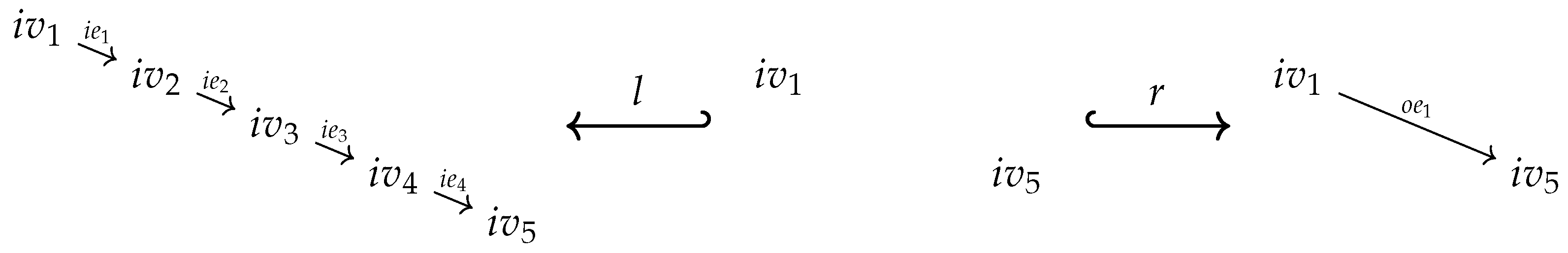
We consider the composition of two morphisms in a category as a graph operation. The arity of a corresponding operation symbol comp could be declared in the following way.
I comp : i v 1 i e 1 i v 2 i e 2 i v 3 O comp : i v 1 o e 1 i v 3
Compared to traditional algebraic operations, we can presently infer some essential differences [7]:
Two 
different kinds of input items. This is evident due to working with graphs that consist of both vertices and edges. Instead of a single set, we therefore declare a graph as the input arity.
Arbitrarily 
many output items. A single output is assumed for algebraic operations, but graph operations can produce arbitrarily large finite graphs as output. Similar to the input, the output arity is chosen to be a graph.
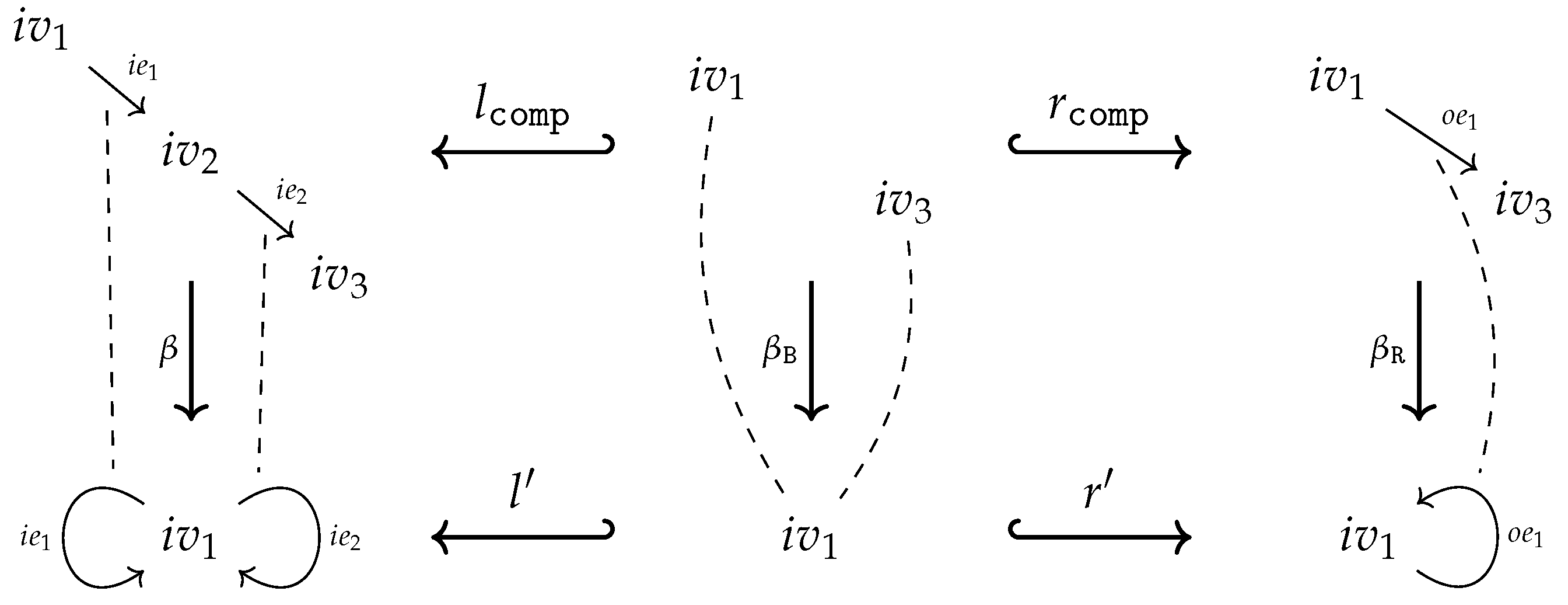
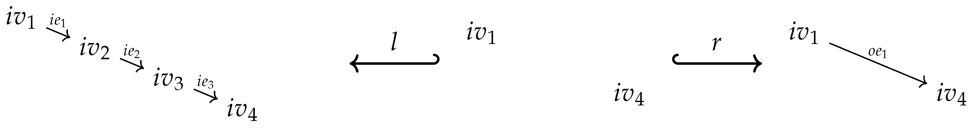
Output 
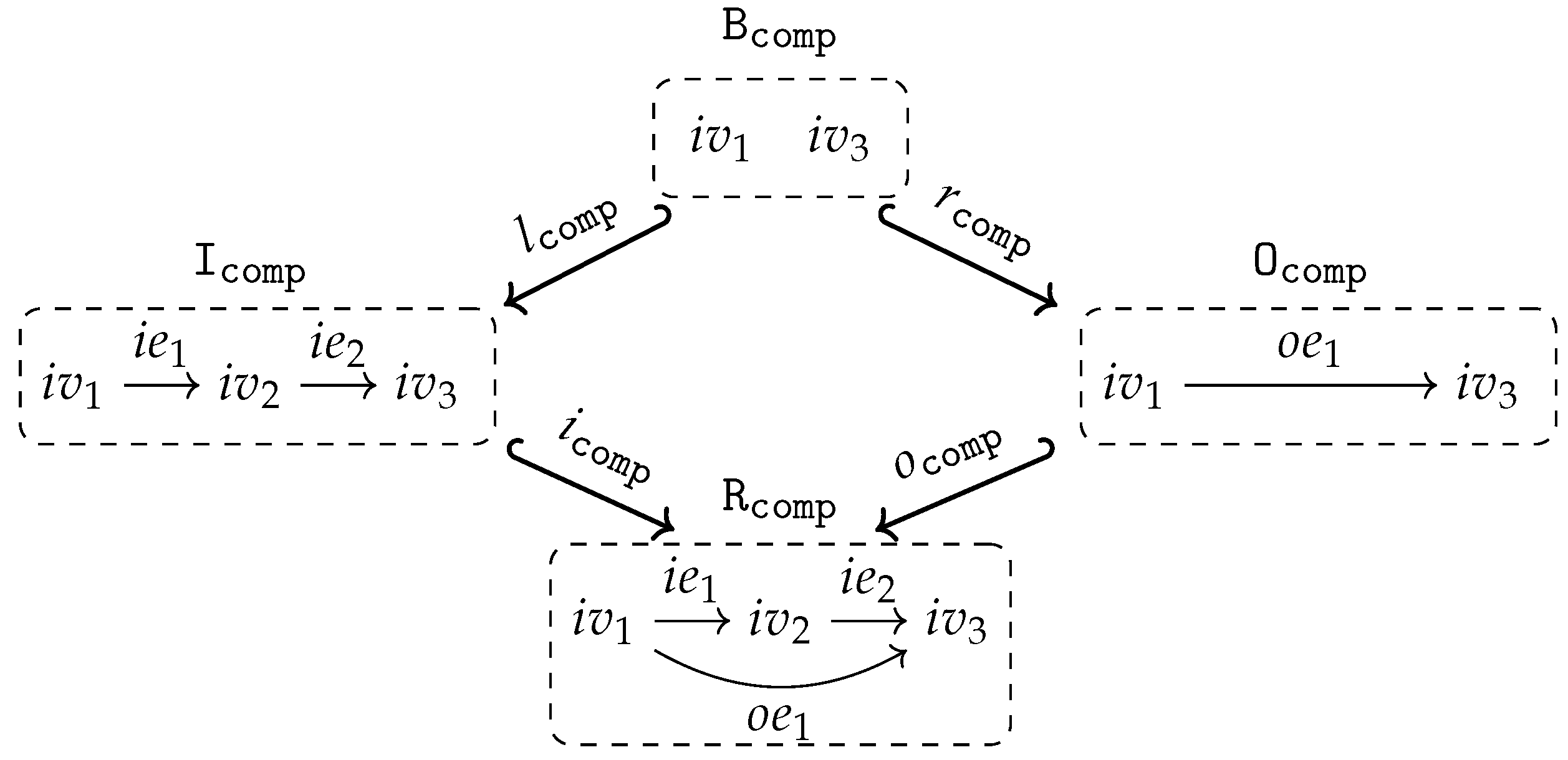
is often related to the input. In the case of the composition operation comp above, the relation between the two arity graphs I comp and O comp is clear from the labelling: the output edge o e 1 has the same source and target as the input edges i e 1 and i e 2 , respectively. Instead of always requiring coherent labeling, we introduce a third arity graph B comp , called the boundary of comp , to encompass the connection between input and output in a fitting way.
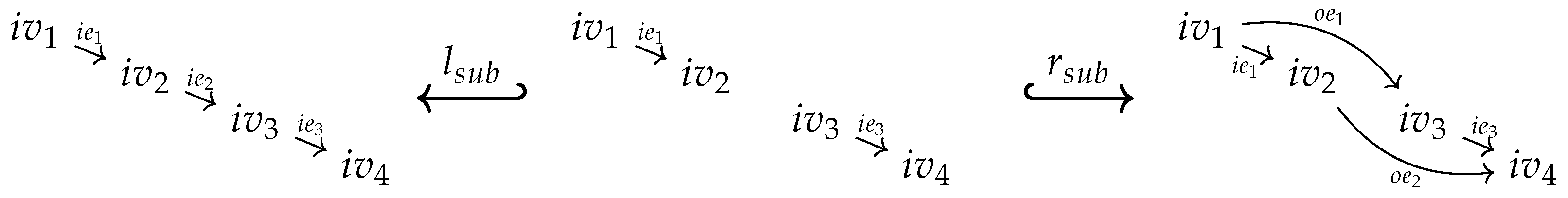
We summarize the previous discussion as the following definition.
Definition 4.1 
(Graph signature). A graph signature Γ = ( O P , a r ) is given by
  • A set O P of operation symbols,
  • A map a r assigning to each operation symbol op in O P its arity span , i.e., a span a r ( op ) = I op l op B op r op O op of inclusion graph homomorphisms between finite graphs such that the sets ( O op ) V ( B op ) V and ( I op ) V as well as the sets ( O op ) E ( B op ) E and ( I op ) E are disjoint. The graphs I op , B op , and O op are referred to as the input arity, boundary arity, and output arity of op , respectively.
If I c is the empty graph 0 for c O P , we also say that c is a constant symbol. Note that B c = 0 in this case.
It is maybe worth mentioning that the disjointedness condition is equivalent to the condition that B op is the componentwise set intersection of the graphs I op and O op , i.e.,
( B op ) V = ( I op ) V ( O op ) V and ( B op ) E = ( I op ) E ( O op ) E .
Remark 4.1 
(Arity Renamings). In contrast to traditional operations, we use explicit names to identify the input and output “positions” of a graph operation. Names can, however, be chosen arbitrarily, and we should be prepared to rename, if necessary, the arities of a graph operation.
An arity renaming ϱ from an arity span I l B r O to another arity span I l B r O is simply a triple of graph isomorphisms ϱ I : I I , ϱ B : B op B , ϱ O : O O such that the following diagram commutes.
Logics 01 00010 i012
Remark 4.2 
(Notational Conventions). For all finite graphs J used in arity spans, we assume that the corresponding sets J V and J E are equipped with a fixed total order. Relying on our conventions in Section 2, this allows us to represent any graph homomorphism b = ( b V , b E ) : J G as a pair of tuples b V = ( b v 1 , , b v n ) , b E = ( b e 1 , , b e m ) , where n = | J V | , m = | J E | and b v i ( b e j ) the image of the i-th (j-th) element in J V ( J E ), 1 i n , 1 j m . For any arity span I l B r O , we assume that B inherits the order from I and O , respectively.
We impose the disjointness condition in Definition 4.1 to syntactically distinguish between input items of a graph operation and the new output items produced by a graph operation. Another objective is to be able to later infer the arity of a “graph operation expression” based only on the expression itself and the arities of the operations symbols defined in the corresponding signature.
To achieve this goal, we will use “canonical arity spans” to describe the arities of operation symbols and graph operation expressions. In a canonical arity span, we use canonical sets I V = { i v 1 , , i v n I } of input vertices and I E = { i e 1 , , i e m I } of input edges with n I = | I V | and m I = | I E | . In the same way, we use canonical sets O V B V = { o v 1 , , o v n O } of output vertices and O E B E = { o e 1 , , o e m O } of output edges with n O = | O V B V | and m O = | O E B E | .
Example 4.1 
(Signature for Categories). We define a signature Γ c a t with an operation symbol comp to denote operations composing two edges and an operation symbol id to denote operations, assigning to vertices corresponding identity edges.
As per Definition 4.1, we extend the arity of   comp   proposed in (14) to the span of graph homomorphisms shown in Figure 1 with a boundary graph   B comp   consisting of only two vertices,   i v 1   and   i v 3   . This encapsulates exactly the desired requirements for a composition operation with regards to sources and targets.
Analogously, the arity of id , shown in Figure 2, encapsulates the requirements for an identity operation with regard to sources and targets.
Graph is a locally small category, and we employ here the same exponential notation for hom-sets as we did for sets in Section 3. That is, for any graphs G and H , G H denotes the set Graph ( H , G ) of all graph homomorphisms from H into G .
Graph operations are maps, i.e., morphisms in Set ! Specifically, an operation op G on a graph G should take as input a graph homomorphism in G I op and return as output a graph homomorphism in G O op . This procedure needs to respect the boundary, which is ensured by requiring the resulting square being commutative.
Definition 4.2 
(Graph Algebra). Let   Γ = ( O P , a r ) be a graph signature. A (graph) Γ -algebra G = ( G , O P G ) is given
  • By a graph   G , called the carrier of G , and
  • By a family   O P G = ( op G : G I op G O op | op O P )   of maps such that the following diagram commutes for all   op   in   O P   and all graph homomorphisms   b G I op .
Logics 01 00010 i013
The maps in   O P G   are referred to as graph operations.
In the specific case where I op is the empty graph 0 , the set G I op becomes a singleton, as there is exactly one graph homomorphism 0 G : 0 G , represented by a pair of empty tuples 0 G = ( ( ) , ( ) ) . Thus, for any constant symbol c in O P , with I c = 0 , the corresponding graph operation c G returns a subgraph of G , i.e., it returns the image of O c under c G ( 0 G ) .
In the case where the signature Γ has no constant symbols, the empty graph constitutes a Γ -algebra, called the empty Γ -algebra.
Example 4.2 
(Categories as Graph Algebras). We consider the graph signature Γ c a t in Example 4.1.
Logics 01 00010 i014
Obviously, any small category   C   gives rise to a   Γ c a t   -algebra   C = ( g r ( C ) , O P C )   with the underlying graph   g r ( C )   of   C   as carrier: the graph operation   comp C : g r ( C ) I comp g r ( C ) O comp   is defined by the single equation   ( comp C ( b ) ) E ( o e 1 ) : = b E ( i e 1 ) ; C b E ( i e 2 )   for all   b g r ( C ) I comp   where “ _ ; C _ ” denotes the composition in   C   . For the two vertices in   O comp   , the images with respect to   comp C ( b )   are always fixed due to the commutativity condition in Definition 4.2:   ( comp C ( b ) ) V ( i v 1 ) = b V ( i v 1 )   and   ( comp C ( b ) ) V ( i v 2 ) = b V ( i v 2 )   .
Not every   Γ c a t   -algebra, however, can be seen as a category, since it may fail to satisfy the identity and/or the associativity law. In [7], we presented some ideas concerning equations for graph algebras, but the development of a full equational calculus is a topic for future research.
Example 4.3 
(Chosen Pullbacks). Graph algebras can serve as a conceptual tool to give a precise meaning to statements like “let C be a category with chosen pullbacks”.
We define the arity of an operation symbol pb as the span of inclusion graph homomorphisms shown in Figure 3. To choose pullbacks for a small category   C   then means nothing but to define a graph operation   pb C : g r ( C ) I pb g r ( C ) O pb   assigning to each cospan   b : I pb g r ( C )   in   C   a corresponding pullback span   pb C : O pb g r ( C )   .
Remark 4.3 
(Built-in Projections). Given a “set of indices” I and a “carrier set” A, we do have a projection map π i : A I A at hand for any index i I , as described in Section 2.
Analogously, we obtain for a “graph of indices”   H   and a “carrier graph”   G   a projection map   π K H   for any subgraph   K   of   H   by simple precomposition with the inclusion graph homomorphism   ι K , H : K H   :
π K H : G H G K i s d e f i n e d b y π K H ( b ) : = ι K , H ; b f o r a l l b G H .
In this way, we do have for any   Γ   -algebra   G = ( G , O P G )   and any arity span   I l B = r O   (as in Definition 4.1) with   B = O   exactly one map from   G I   to   G O   satisfying the commutativity condition for graph operations in Definition 4.2, namely the projection   π O I : G I G O   . In case   I = B = O   ,   π I I : G I G I   is simply the identity on   G I   .
We call these projections built-in since their semantics is completely determined by their arity! After the choice of the carrier G of a graph algebra G we do have these projections available independent of and prior to the choice of the semantics op G of the operation symbols op O P .
A crucial methodological point is that we can use these built-in projections without being forced to include corresponding auxiliary operational symbols in   O P   and/or without any need to define their semantics when defining graph algebras. In the traditional approach, we are forced to do this because there is no concept of boundaries at all, or, in other words, all boundaries in our sense are by default empty in traditional Universal Algebra.
Our reformulation of the definition of homomorphisms for traditional algebras in Definition 3.3 applies analogously to graph algebras.
Definition 4.3 
(Graph Algebra Homomorphism). Let Γ be a graph signature. A Γ -homomorphism φ : G H between two Γ -algebras G = ( G , O P G ) and H = ( H , O P H ) is a graph homomorphism φ : G H satisfying the following homomorphism condition:
( HC ) op G ( b ) ; φ = op H ( b ; φ ) f o r a l l op O P a n d a l l b G I op
Logics 01 00010 i015
For any graphs G , H , and J each graph homomorphism φ : G H induces by postcomposition a map _ ; φ : G J H J and thus we can, more abstractly but equivalently, express the homomorphism condition (HC) via the requirement that the above right square of maps commutes. Note that in the case of constant symbols c O P , I c = 0 , the homomorphism condition turns into the equation op G ( ( ) , ( ) ) ; φ = op H ( ( ) , ( ) ) if we apply our conventions in Section 2 and Remark 4.2 concerning the tuple notation.
Example 4.4 
(Functors as Homomorphisms). In the case of Γ c a t -algebras as defined in Example 4.2, the homomorphism conditions for the operation symbols comp and id , according to Definition 3.3, are nothing but the usual requirements for functors to be compatible with composition and identities, respectively.
Γ -algebras and Γ -homomorphisms together constitute a category Alg ( Γ ) : The composition φ ; ψ : G K of two Γ -homomorphisms φ : G H and ψ : H K is given by the composition φ ; ψ of the underlying graph homomorphisms φ : G H and ψ : H K . Lastly, the identity Γ -homomorphism i d G : G G for any Γ -algebra G is given by the identity graph homomorphism i d G : G G .
Proposition 4.1 
(Forgetful Functor). The assignments G G and ( φ : G H ) ( φ : G H ) define a faithful forgetful functor:
U Γ : Alg ( Γ ) Graph .
The homomorphism condition for Σ -homorphisms between Σ -algebras in Definition 3.3 has exactly the same structure as the homomorphism condition for Γ -homomorphisms between graph Γ -algebras in Definition 4.3. In such a way, the pure categorical proof of Theorem 3.1 can be directly transformed into a proof of the corresponding statement for graph algebras, and thus, we obtain the following theorem “for free”.
Theorem 4.1 
(Limits of Graph Algebras). Alg ( Γ ) inherits any small limit from the category Graph , i.e., the functor U Γ : Alg ( Γ ) Graph creates small limits. Alg ( Γ ) therefore has all small limits since Graph does.

4.2. Comparison with the Old Definitions

Guided by the pioneering generalized sketch framework developed in the 1990s by a group around Zinovy Diskin [3,4,5], we introduced in [7] a different definition of graph signatures and graph algebras, respectively. Ref. [7] considers a graph inclusion i op : I op R op as the arity of an operation symbol op and defines an operation op G on a graph G as a map from G I op to G R op , making the following triangle commute for any b : I op G .
Logics 01 00010 i016
The need for projection operations, among other issues, advised us to introduce explicit output arities. At that point, we could have also chosen cospans I op R op O op to declare the arities of graph operations instead of the spans in Definition 4.1. The choice of spans has, however, many advantages that we will try to point at later in the paper.
In this subsection, we argue that the new variant and the old variant in [7] are semantically equivalent as either definition of arity, algebra, or homomorphism can be obtained from the other.

4.2.1. Comparison of Arity Declarations

For any arity span I op l op B op r op O op in Definition 4.1, we can simply construct a pushout to obtain the result arity R op
Logics 01 00010 i017 
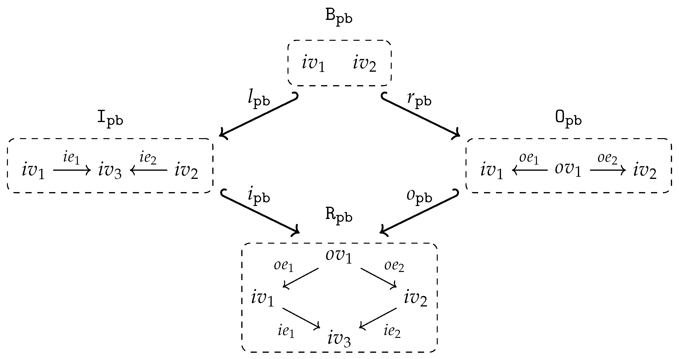
The pushout of the arities of the operation symbol comp is visualized in Figure 4.
Pushouts in Graph (as in any topos) preserve monomorphisms, and, moreover, pushouts with a monomorphism involved are also pullbacks ([16], 13.3). Equation (15) ensures that we can choose the specific pushout R op = I op O op , which makes the resulting i op into a graph inclusion, matching the definition in [7]. Note that B op = O op implies I op = R op .
Conversely, given a cospan I op i op R op o op O op of graph inclusions, we can construct the intersection B op = I op O op , i.e., the componentwise intersection of the vertex and edge sets. This is well-defined as both I op and O op are subgraphs of the same graph R op . The resulting commutative square of inclusion graph homomorphisms is a pullback in Graph where the span I op l op B op r op O op satisfies the condition in Definition 4.1. In the case where R op = I op O op , the square is also a pushout!
Arities of graph operations are, however, defined in [7] by a single graph inclusion i op : I op R op only. In this situation, we can construct a cospan I op i op R op o op O op of graph inclusion with O op the smallest subgraph of R op containing all vertices in ( R op ) V \ ( I op ) V and all edges in ( R op ) E \ ( I op ) E . By construction, we have R op = I op O op . As for cospans, in general, B op is defined to be the graph I op O op . However, the crucial observation is that B op will always be a discrete graph, i.e., a graph without edges! Note that this construction is a special case of the construction of so-called initial pushouts in Graph ([9], 6.1).
Since, for a pushout of arities, B op = O op implies I op = R op , this means, especially, that the original definition of arities of graph operations in [7] does not allow us to consider built-in projections (see Remark 4.3) as legal graph operations. This was one of the main reasons that we introduced spans of graph inclusions as arities in this paper.
In conclusion, the span and cospan version are inverse to each other (at least in Graph ) while the original version in [7] is a special case of the cospan version, which is less expressive than the other two versions. All three variants give us, however, a pushout of arities and inclusion graph homomorphisms at hand.

4.2.2. Equivalence of Graph Operations

Given a pushout of arities, we consider an arbitrary input b : I op G .
Logics 01 00010 i018 For any o : O op G with r op ; o = l op ; b , there exists, due to the pushout property, a unique r o : R op G with i op ; r o = b and o op ; r o = o . Conversely, for any r : R op G with i op ; r = b , we have, trivially, l op ; b = r op ; ( o op ; r ) .
The uniqueness of mediating morphisms ensures that the assignments o r o and r o op ; r are inverse to each other. This observation ensures that there is a one-to-one correspondence between maps from G I op to G R op , satisfying commutativity condition (19), and maps from G I op to G O op , satisfying the commutativity condition in Definition 4.2.

4.2.3. Equivalence of Homomorphism Conditions

By extending the equivalence of graph operations, the equivalence of the respective homomorphism conditions can also be straightforwardly shown utilizing the uniqueness of mediating morphisms for the pushout of arities, as the interested reader may check.
Remark 4.4 
(Graph of a Graph Operation). For any map f : A B , its graph is usually defined as the binary relation { ( a , f ( a ) ) a A } A × B . Often, the story is even turned, and maps are introduced as those binary relations f A × B that are left-total and right-unique.
Given a pushout of arities and a graph operation   op G : G I op G O op   , we could, analogously, consider the set   { r op G ( b ) b G I op } G R op   as the graph of the graph operation   op G   . Utilizing the projections from   G R op   into   G I op   and   G O op   , we could even lift up properties like left-total and right-unique to characterize those subsets of   G R op   that correspond to graph operations.
This observation may be a basis for defining Skolemization in Logics of Statements in Context [1] once we have integrated operations into those logics.
R op   also has another important role, which was probably one of the reasons that the original definition of sketch operations in [3,4,5] relied on graph inclusions   i op : I op R op   .   R op   is the only place where the input items of a graph operation and the new items, created by the graph operation, can be related. In such a way, we have to use   R op   if we want to describe and specify properties of the output of a graph operation that depend on properties of the input.
Example 4.5 
(Graph of Pullback Operation). Figure 5 shows the pushout of arity declarations for the operation symbol pb . Constructing the graph of pullback operations, as described in Example 3, considers for any chosen pullback the whole pullback square, and not just the pullback span.
Example 4.6 
(Chosen (co)limits). In general, any chosen (co)limits of diagrams of a fixed shape I in a category C give rise to a corresponding graph operation on g r ( C ) where the arity B is simply given by all the vertices in I while arity O represents the shape of the corresponding (co)cones.
In such a way, the pushout   R   combines the fixed shape   I   of diagrams with the shape of corresponding (co)cones, and thus, the elements in the graph of the corresponding graph operation on   g r ( C )   represent, at the same time, a diagram and a (co)cone for this diagram.
Remark 4.5 
(Advantages of Spans of Arities). Starting with a span of arities as in Definition 4.1, we obtain a corresponding commutative square of arities via a simple pushout construction. That this square becomes, moreover, in any topos, a pullback is an essential side effect.
If we start, in contrast, with a cospan, we could construct a pullback to obtain a commutative square of arities. In the case of graphs (and probably in arbitrary pre-sheaf topoi), it is sufficient to require that the cospan of inclusion morphisms is jointly epic to make the pullback square simultaneously a pushout square. We are, however, not sure that this condition is sufficient for arbitrary topoi.
The tricky construction of initial pushouts for a single arity inclusion (and not a cospan!) may also generalize to arbitrary pre-sheaf topoi but probably not to arbitrary topoi.
The original definition of arities and graph operations in [7] turned out to not be appropriate to define derived graph operations. On one hand, projections are necessary to define an appropriate notion of derived graph operations. The original definition excludes, however, projections. On the other hand, the construction of instances of graph operations in Section 5.3.2, by means of epi-mono factorizations and pushouts, cannot equivalently be mimicked by means of the original definition. Even the universal property of initial pushouts is not helpful in establishing an equivalence.

4.3. Graph Subalgebras

The definitions and results for graph algebras presented in this subsection are new and not found in [7].
The effort we spent in Section 3 to lift up the traditional exposition of algebras to a more categorical one pays off now. We can directly transfer most of the definitions and results from algebras to graph algebras. The only difference is that the “ad hoc totalization trick” in the proof of Proposition 3.3 does not work in the case of graph algebras and that there is no axiom of choice in Graph .
In contrast to Section 3, we do not distinguish between “subalgebras” and “inclusion homomorphisms”. We define “subalgebras” simply as “inclusions”.
Definition 4.4 
(Graph Subalgebra). Let Γ = ( O P , a r ) be a graph signature. A Γ -algebra G = ( G , O P G ) is a Γ -subalgebra of a Γ -algebra H = ( H , O P H ) if G H and and the inclusion graph homomorphism ι G , H = ( ι G V , H V , ι G E , H E ) : G H establishes a Γ -homomorphism ι G , H : G H .
We know that the monomorphisms (epimorphisms) in Graph are exactly the injective (surjective) graph homomorphisms, respectively. Since the functor U Γ : Alg ( Γ ) Graph is faithful and faithful functors reflect monomorphisms and epimorphisms, we obtain
Corollary 4.1 
(Injective and surjective Homomorphisms). If the underlying graph homomorphism φ : G H of a Γ -homomorphism φ : G H is injective (surjective), then φ : G H is a monomorphism (epimorphism) in Alg ( Γ ) .
The category Graph has all small limits and colimits, and those are obtained by componentwise limits and colimits, respectively, in Set . This means, especially, that Graph has all small multiple pullbacks (see Remark 3.3). Due to Theorem 4.1, we can define, in such a way, the intersection of graph subalgebras analogous to the intersection of subalgebras in Corollary 3.3.
Corollary 4.2 
(Intersection of Graph Subalgebras). For any set I, any Γ -algebra H , and any diagram δ : MP ( I ) Alg ( Γ ) of Γ -subalgebras δ e i = ι G i , H : G i H , i I of H there is a unique Γ -subalgebra L = ( L , O P L ) of H with L = i I G i , i.e., L V = i I ( G i ) V and L E = i I ( G i ) E , that is a Γ -subalgebra of G i for all i I .
Moreover, the inclusion   Γ   -homomorphisms   ι L , G i : L G i   ,   i I   and   ι L , H : L H   constitute a multiple pullback, i.e., a limit cone of the diagram   δ : MP ( I ) Alg ( Γ )   .
We call   L = ( L , O P L )   also the intersection of the I-indexed family   M = ( G i i I )   of   Γ   -subalgebras of   H   and may use the notations   M   ,   i I G i   or, simply,   G i   to denote   L   .
The category Graph is well powered; i.e., the collection of all graph subalgebras of a graph algebra is a set, and thus, we can define the concept “accessible via a graph homomorphism”.
Definition 4.5 
(Graph Subalgebra accessible via a Graph Homomorphism). For any   Γ   -algebra   H   and any graph homomorphism   φ : G H   , let   M   be the set of all   Γ   -subalgebras   X   of   H   such that   φ   factors through the inclusion graph homomorphism   ι X , H : X H   ; i.e., there exists a graph homomorphism   φ X : G X   such that   φ X ; ι X , H = φ   .
We denote by   R ( φ , H )   the intersection of   M   , according to Corollary 4.2. In particular, the carrier of   R ( φ , H )   is the intersection   R ( φ , H ) : = { X X M }   of graphs. We call   R ( φ , H )   the   Γ   -subalgebra of   H   accessible (reachable) via   φ   or the homomorphic image of   G   with respect to   φ   .
In the case of inclusion graph homomorphisms   φ = ι G , H : G H   , we also use the notation   R ( G , H )   instead of   R ( ι G , H , H )   and also call   R ( G , H )   the Γ -subalgebra of   H   generated by   G   .
Note that the graph homomorphism φ X : G X in Definition 4.5 is unique, if it exists, since the inclusion graph homomorphism ι X , B : X H is a monomorphism in Graph .
We can also transfer Corollary 3.4 to graph algebras since, for any graph homomorphism φ : G H , the set-theoretic image φ ( G ) of G with respect to φ constitutes a subgraph of H . Moreover, we have φ ( G ) = { Y Y N } for the set N of all subgraphs Y of H .
Corollary 4.3 
(Homomorphic image includes Image). For any Γ -algebra H and any graph homomorphism φ : G H , we have φ ( G ) R ( φ , H ) for the set-theoretic image φ ( G ) of G with respect to φ .
Definition 4.6 
(Accessible and Generated Graph Algebras). Let H be a Γ -algebra.
1. 
  H   is accessible via a graph homomorphism   φ : G H   if   R ( φ , H ) = H   .
2. 
If   H   is accessible via an inclusion graph homomorphism   ι G , H : G H   , i.e., if   R ( G , H ) = R ( ι G , H , H ) = H   , we say also that   H   is generated by   G   .
3. 
  H   is said to be generated if it is generated by the empty graph, i.e., accessible via the unique graph homomorphism   ι 0 , H : 0 H   from the initial object   0   in   Graph   to   H   .
Corollary 4.4. 
A   Γ   -algebra   H   is generated if, and only if, there are no proper   Γ   -subalgebras of   H   .
Corollary 4.5. 
If a signature   Γ   has no constant symbols, then the empty   Γ   -algebra is the only generated   Γ   -algebra.
The concept accessible via a graph homomorphism can be utilized to find a characterization of epimorphisms in Alg ( Γ ) . First, we observe that “accessible” implies “epic”.
Lemma 4.1 
(Accessible implies Epic). A Γ -homomorphism φ : G H is an epimorphism in Alg ( Γ ) if H is accessible via the underlying graph homomorphism φ : G H , i.e., if H = R ( φ , H ) .
Proof. 
We consider arbitrary Γ -homomorphsms ψ , ϕ : H K such that φ ; ψ = φ ; ϕ .
We know that the subgraph X of H with X V = { v H V ψ V ( v ) = ϕ V ( v ) } H V , X E = { e H E ψ E ( e ) = ϕ E ( e ) } H E together with the inclusion graph homomorphism ι X , H : X H is an equalizer of the graph homomorphisms ψ , ϕ : H K in Graph . According to Theorem 4.1, there is a unique Γ -algebra X = ( X , O P X ) such that ι X , H : X H becomes an inclusion Γ -homomorphism ι X , H : X H , which is, moreover, the equalizer of the Γ -homomorphisms ψ , ϕ : H K .
The assumption φ ; ψ = φ ; ϕ ensures that there exists a unique graph homomorphism φ X : G X with φ X ; ι X , H = φ . Due to the construction of R ( φ , H ) in Definition 4.5, we have an inclusion Γ -homomorphism ι R ( φ , H ) , X : R ( φ , H ) X .
The accessibility of H means H = R ( φ , H ) , and thus, we obtain, finally, X = H . This means, however, that the equalizer of ψ and ϕ in Graph is the identity on H and thus, we have ψ = ϕ as required. □
We can also show that graph subalgebras are regular monomorphisms. Unfortunately, the “ad hoc totalization trick”, used in the proof of Proposition 3.3, does not work for arbitrary graph operations, since we may have, in contrast to traditional operations, non-empty boundaries and a corresponding commutativity requirement for graph operations. The simplest example, where this trick fails, is an operation that simply outputs a chosen edge between two distinct nodes.
What we need is a more well-behaved procedure of transforming partial graph algebras into total graph algebras. We therefore develop in Section 4.4 a corresponding free construction called term completion.
Proposition 4.2 
(Graph Subalgebras are Regular Monos). For any Γ -subalgebra ι G , H : G H of a Γ -algebra H there exists a Γ -algebra K and parallel Γ -homomorphisms ψ , ϕ : H K such that ι G , H : G H is the equalizer of ψ and ϕ in Alg ( Γ ) .
Proof. 
Utilizing the term completion construction and its characterization as a free construction, as presented in Section 4.4, we will sketch a proof modifying the proof of Proposition 3.3.
We construct the pushout of the span H l G , H G l G , H H of inclusion graph homomorphisms (see the left diagram below). We set K : = H + G H . Since ι G , H is monic in Graph both graph homomorphisms κ 1 , κ 2 : H K are monic too and, moreover, the pushout square is as a pullback square as well. This ensures, especially, that ι G , H : G H is the equalizer of the graph homomorphisms κ 1 , κ 2 : H K in Graph .
Logics 01 00010 i019Graph Operations on K : We extend K to a partial Γ -algebra K = ( K , O P K ) (see Definition 4.7) by defining for each op in O P a corresponding partial graph operation op K : K I op K O op according to Case 1, Case 2, and Case 3.
The operations in K are defined exactly in a way that the graph homomorphisms κ 1 and κ 2 become Γ -homomorphisms κ 1 , κ 2 : H K , in the sense of Definition 4.8, and thus we obtain a commutative square in PAlg (see the middle diagram above).
Applying the functor TC Γ : PAlg ( Γ ) Alg ( Γ ) , we transform this commutative square in PAlg ( Γ ) into a commutative square in Alg ( Γ ) . Taking into account Corollary 4.6 and (23), we obtain the commutative diagram on the right above.
The underlying square of graph homomorphisms is again a pullback in Graph since the inclusion graph homomorphism ι K , T Γ ( K ) : K T Γ ( K ) is monic in Graph .
Theorem 4.1 ensures, finally, that the Γ -homomorphism ι G , H : G H is the equalizer of the Γ -homomorphisms κ 1 ; ι K , T Γ ( K ) , κ 2 ; ι K , T Γ ( K ) : H T Γ ( K ) . □
The regularity of Alg ( Γ ) entails that the concepts accessible and epic are equivalent.
Proposition 4.3 
(Accessible ≅ Epic). For any Γ -homomorphism φ : G H , it holds that H is accessible via the underlying graph homomorphism φ : G H ; i.e., in other words, H is equal to the homomorphic image R ( φ , H ) of G with respect to φ , if, and only if, φ : G H is an epimorphism in Alg ( Γ ) .
Proof. 
“Accessible implies epic” has been shown in Lemma 4.1. We show now that “epic implies accessible”: We consider an arbitrary Γ -subalgebra X of H such that there exists a graph homomorphism φ X : G X with φ X ; ι X , B = φ . Due to Proposition 4.2, there exist Γ -homomorphisms ψ , ϕ : H C such that ι X , H : X H is the equalizer of ψ and ϕ . Due to the assumption φ X ; ι X , H = φ , we obtain φ ; ψ = φ ; ϕ and thus ψ = ϕ , since φ is epic. This means, however, that X = H and, finally, R ( φ , H ) = H due to the construction of R ( φ , H ) in Definition 4.5. □
The axiom of choice is not valid in Graph . Therefore, the set-theoretic image φ ( G ) of the carrier G of a Γ -algebra G with respect to a Γ - homomorphism φ : G H is, in general, not closed with respect to operations in H . As a consequence, not every epic Γ -homomorphism needs to be surjective. We adapt the standard example of the composition of morphisms in categories.
Example 4.7 
(Epic ≇ Surjective). We consider a Γ c a t -homomorphism φ : G H between two finite Γ c a t -algebras G and H , as depicted below.
Logics 01 00010 i020
G I comp   is empty, while   H I comp   has exactly one element   b   given by the assignments   f α   ,   g β   .   α   and   β   are in the set-theoretic image   φ ( G )   , while the result of applying   comp G   to   b   , namely   γ = comp G ( b ) ( o e 1 )   , is not.   φ : G H   is not surjective but epic since   H = R ( φ , H )   .

4.4. Partial Graph Algebras and Their Term Completion

In practice, graph operations are often partial graph operations. The sketch operations introduced in [4,5], for example, can be seen as partial graph operations where the domain of definition is specified by diagrammatic predicates. Therefore, we have decided to also present in this paper the very basic definitions for partial graph algebras.
This decision was also influenced by the observation that we could prove Proposition 4.2 for arbitrary graph signatures based on a well-behaved completion procedure transforming partial (graph) algebras into total (graph) algebras. To our surprise, the construction of (graph) term algebras turns out to be just a special case of this new procedure.
Definition 4.7 
(Partial Graph algebra). A partial (graph)   Γ   -algebra   G   is a pair   ( G , O P G )   given
  • By a graph   G   , called the carrier of   G   , and
  • By a family   O P G = ( op G : G I op G O op | op O P )   of partial maps such that the following diagram commutes for all   op   in   O P   and all graph homomorphisms   b d o m ( G I op )   .
Logics 01 00010 i021
The partial maps in O P G are referred to as partial graph operations.
Be aware that constants can also be partial! For any constant symbol c in O P , with I c = 0 , we do have exactly two possibilities, since G I c is a singleton: Either d o m ( c G ) = G I c , i.e., the constant is defined, or d o m ( c G ) = , i.e., the constant is not defined.
Definition 4.8 
(Partial Graph Algebra Homomorphism). A Γ -homomorphism φ : G H between two partial Γ -algebras G = ( G , O P G ) and H = ( H , O P H ) is a graph homomorphism φ : G H satisfying the following homomorphism condition
( HCP ) b ; φ d o m ( H I op ) a n d op G ( b ) ; φ = op H ( b ; φ ) f o r a l l op O P a n d a l l b d o m ( G I op ) .
Logics 01 00010 i022
In other words, the definedness of partial operations has to be preserved by a homomorphism but does not need to be reflected!
Partial graph Γ -algebras and Γ -homomorphisms between them constitute a category PAlg ( Γ ) : The composition φ ; ψ : G K of two Γ -homomorphisms φ : G H and ψ : H K is given by the composition φ ; ψ of the underlying graph homomorphisms φ : G H and ψ : H K . The identity Γ -homomorphism i d G : G G for any partial Γ -algebra G is given by the identity graph homomorphism i d G : G G . We consider graph Γ -algebras as special partial Γ -algebras and thus Alg ( Γ ) is a full subcategory of PAlg ( Γ ) .
Proposition 4.4 
(Forgetful Functor). The assignments G G and ( φ : G H ) ( φ : G H ) define a faithful forgetful functor
U Γ P : PAlg ( Γ ) Graph .
By introducing a fresh new element whenever an operation is not defined for a certain input, we can transform any partial (graph) algebra into a total (graph) algebra.
Remark 4.6 
(Syntactic Representation of Inputs). In addition to our notational conventions in Section 2 and Remark 4.2, we will rely on the following syntactic representation of inputs of graph operations: For any graph G and any op in O P an input b = ( b V , b E ) G I op is represented by two strings, representing the vertices and the edges in G , respectively, separated by the symbol “|”
s y n ( b ) : = b v 1 , , b v n op | b e 1 , , b e m op
where n op = | ( I op ) V | and m op = | ( I op ) E | . In the case I op = 0 , the only the input 0 G = ( ( ) , ( ) ) : 0 G is represented, in such a way, by two separated empty sequences: s y n ( 0 G ) = | .
Of course, we could work with any other syntactic representation as long as the following two important properties are satisfied: (1) Uniqueness, i.e., for all   b 1 , b 2 G I op   we have   s y n ( b 1 ) = s y n ( b 2 )   if, and only if,   b 1 = b 2   ; (2)   s y n ( b )   is indeed a representation, i.e., we are able to reconstruct from   s y n ( b )   the corresponding graph homomorphism   b = ( b V , b E ) G I op     with the help of the information about   I op   in the signature   Γ   . In the case where   I op   has no isolated vertices, for example, we can uniquely represent any   b G I op   by the string   b e 1 , , b e m op   only!
Definition 4.9 
(Term Completion). Let Γ = ( O P , a r ) be a graph signature and K = ( K , O P K ) be a partial Γ -algebra. We define the Γ -term completion T Γ ( K ) of the graph K with respect to the partial Γ -algebra K as the smallest graph satisfying the following three conditions:
Generators: 
K T Γ ( K )
Constants: 
For all constants   c   in   O P   , such that   d o m ( c K ) =   , the graph   T Γ ( K )   contains
  •   c o v |   as a vertex, for each vertex   o v   in   O c   ;
  •   c o e |   as an edge, for each edge   o e   in   O c   , where   s c T Γ ( K ) ( c o e | ) : = c s c O c ( o e ) |   and   t g T Γ ( K ) ( c o e | ) : = c t g O c ( o e ) |  
Operations: 
For all op in   O P   with   I op 0   and any   t T Γ ( K ) I op   such that there is no   b d o m ( op K ) K I op   with   t = b ; ι K , T Γ ( K )   ,   T Γ ( K )   contains
  • op o v s y n ( t )   as a vertex, for each vertex   o v   in   ( O op ) V ( B op ) V   ;
  •   op o e s y n ( t )   as an edge, for each edge   o e   in   ( O op ) E ( B op ) E   , where
s c T Γ ( K ) ( op o e s y n ( t ) ) : = t V ( s c O op ( o e ) ) , i f s c O op ( o e ) ( B op ) V op s c O op ( o e ) s y n ( t ) , i f s c O op ( o e ) ( O op ) V ( B op ) V
t g T Γ ( K ) ( op o e s y n ( t ) ) : = t V ( t g O op ( o e ) ) , i f t g O op ( o e ) ( B op ) V op t g O op ( o e ) s y n ( t ) , i f t g O op ( o e ) ( O op ) V ( B op ) V
Obviously, we have
T Γ ( K ) = K for all total Γ - algebras K = ( K , O P K ) .
Remark 4.7 
(Term Construction by Pushouts). The construction of Γ -terms in Definition 4.9 can be organized as a successive application of term-construction steps starting with the graph K : A term-construction step in the case Constants means that we construct, in parallel, for a constant symbol c the terms for all vertices and edges in O c . Analogously, a term-construction step in the case Operations means that we construct for an operation symbol op and an input t , in parallel, the terms for all vertices and edges in O op B op . Each term-construction step extends an intermediate graph T to a graph T . This extension is, however, nothing but the construction of the following pushout:
Logics 01 00010 i023where the definition of op T Γ ( K ) ( t ) is spelled out, explicitly, in Definition 4.10. In light of this observation, one can look at the term notation as a means to solve two problems:
1. 
The term notation provides a uniform mechanism to create unique identifiers for the new graph items introduced by applying a non-deleting injective graph -transformation rule [9].
2. 
At the same time, the term notation encodes all the information necessary to uniquely identify the pushout that has been creating the new items.
The following term-completion construction is new and has never even been defined for traditional partial algebras. Utilizing the operations in K to the greatest possible extent, we can straightforwardly extend K to a total Γ -algebra with carrier T Γ ( K ) .
Definition 4.10 
(Term-Completion Algebra). We can extend any partial Γ -algebra K = ( K , O P K ) to a total Γ -algebra T Γ ( K ) = ( T Γ ( K ) , O P T Γ ( K ) ) as follows:
Constants: 
For all constants   c   in   O P   :
Utilizing   K   : 
If   c K   is defined, we simply reuse it:
  c T Γ ( K ) ( 0 T Γ ( K ) ) = c T Γ ( K ) ( 0 K ; ι K , T Γ ( K ) ) : = c K ( 0 K ) ; ι K , T Γ ( K )  
Completion: 
If   c K   is not defined, i.e.,   d o m ( c K ) =   we set
  • ( c T Γ ( K ) ( 0 T Γ ( K ) ) ) V ( o v ) : = c o v   for each vertex   o v   in   O c   and
  •   ( c T Γ ( K ) ( 0 T Γ ( K ) ) ) E ( o e ) : = c o e   for each edge   o e   in   O c   .
Operations: 
For all   op   in   O P   with   I op 0   and any   t T Γ ( K ) I op   :
Utilizing   K   : 
If there is a   b d o m ( op K ) K I op   with   t = b ; ι K , T Γ ( K )   , we reuse   op K   :
  op T Γ ( K ) ( t ) = op T Γ ( K ) ( b ; ι K , T Γ ( K ) ) : = op K ( b ) ; ι K , T Γ ( K )  
Completion: 
If there is no   b d o m ( op K ) K I op   with   t = b ; ι K , T Γ ( K )   , we set
  ( op T Γ ( K ) ( t ) ) V ( o v ) : = t V ( o v ) , i f o v ( B op ) V op o v s y n ( t ) , i f o v ( O op ) V ( B op ) V  
  ( op T Γ ( K ) ( t ) ) E ( o e ) : = t E ( o e ) , i f o e ( B op ) E op o e s y n ( t ) , i f o e ( O op ) E ( B op ) E .  
The definitions ensure that the constructed pairs op T Γ ( K ) ( t ) of maps are indeed graph homomorphisms and that the operations in T Γ ( K ) satisfy the commutativity condition in Definition 4.2. Moreover, the cases “Utilizing K ” are defined in such a way that we obtain
Corollary 4.6 
(Embedding). For any partial Γ -algebra K = ( K , O P K ) , the inclusion graph homomorphism ι K , T Γ ( K ) : K T Γ ( K ) constitutes a Γ -homomorphism ι K , T Γ ( K ) : K T Γ ( K ) in PAlg ( Γ ) , and thus, due to (21), T Γ ( K ) = K if K is a total Γ -algebra.
We can adapt and generalize the proof of Proposition 2 (Free graph algebras) in [7] to a proof that term completion is a free construction.
Proposition 4.5 
(Term Completion as a Free Construction). For any partial Γ -algebra K = ( K , O P K ) , the total Γ -algebra T Γ ( K ) = ( T Γ ( K ) , O P T Γ ( K ) ) has the following universal property: for any total Γ -algebra G = ( G , O P G ) and any Γ -homomorphism φ : K G there exists a unique Γ -homomorphism φ : T Γ ( K ) G such that the defining condition ι K , T Γ ( K ) ; φ = φ is satisfied.
Logics 01 00010 i024
Proof. 
We prove this by structural induction according to Definition 4.9 and Remark 4.7.
Generators: 
In this base case, the defining condition forces φ V ( k v ) = φ V ( k v ) for all k v K V and φ E ( k v ) = φ E ( k e ) for all k e K E .
Constants: 
In the second base case, we have, for all constants c in O P :
Utilizing   K : 
If c K is defined, the definition of operations in T Γ ( K ) , the defining condition and the assumption that φ is a Γ -homomorphism ensure that φ satisfies the homorphism condition for the constant c :
c T Γ ( K ) ( 0 T Γ ( K ) ) ; φ = c K ( 0 K ) ; ι K , T Γ ( K ) ; φ = c K ( 0 K ) ; φ = c G ( 0 K ; φ ) = c G ( 0 K ; ι K , T Γ ( K ) ; φ ) = c G ( 0 T Γ ( K ) ; φ )
Completion: 
If c K is not defined, the definition of operations in T Γ ( K ) and the required homomorphism condition for φ forces for each vertex o v in O c
φ V ( c o v | ) = φ V ( c T Γ ( K ) ( 0 T Γ ( K ) ) ) V ( o v ) = c T Γ ( K ) ( 0 T Γ ( K ) ) ; φ V ( o v ) = ( c G ( 0 T Γ ( K ) ; φ ) ) V ( o v ) = ( c G ( 0 G ) ) V ( o v ) .
For each edge o e in O c we obtain, analogously, φ E ( c o e | ) = ( c G ( 0 G ) ) E ( o e ) .
Operations: 
We have, for all op in O P with I op 0 and any t T Γ ( K ) I op ,
Utilizing   K : 
If there is a b d o m ( op K ) K I op with t = b ; ι K , T Γ ( K ) , then the definition of operations in T Γ ( K ) , the defining condition and the assumption that φ is a Γ -homomorphism ensure that φ satisfies the homomorphism condition for t :
op T Γ ( K ) ( t ) ; φ = op K ( b ) ; ι K , T Γ ( K ) ; φ = op K ( b ) ; φ = op G ( b ; φ ) = op G ( b ; ι K , T Γ ( K ) ; φ ) = op G ( t ; φ )
Completion: 
If there is no b d o m ( op K ) K I op with t = b ; ι K , T Γ ( K ) , the induction hypothesis is that φ is already defined on a subgraph T T Γ ( K ) and that t ( I op ) T . This ensures t ; φ G I op . In the induction step, we extend φ to the graph T T Γ ( K ) . The definition of operations in T Γ ( K ) and the required homomorphism condition for φ forces for each vertex o v in ( O op ) V ( B op ) V
φ V ( op o v s y n ( t ) ) = φ V ( op T Γ ( K ) ( t ) ) V ( o v ) = op T Γ ( K ) ( t ) ; φ V ( o v ) = ( op G ( t ; φ ) ) V ( o v ) .
For each edge o e in ( O op ) E ( B op ) E we obtain, analogously, φ E ( op o e s y n ( t ) ) = ( op G ( t ; φ ) ) E ( o e ) .
. □
The assignments K T Γ ( K ) and ( ψ : L K ) ( ( ψ ; ι K , T Γ ( K ) ) : T Γ ( L ) T Γ ( K ) ) define, as usual for free constructions, a functor TC Γ : PAlg ( Γ ) Alg ( Γ ) , and this functor is left-adjoint to the inclusion functor I : Alg ( Γ ) PAlg ( Γ ) .
Logics 01 00010 i025
Due to Corollary 4.6 we even have I ; TC Γ = i d Alg ( Γ ) , i.e., Alg ( Γ ) is a full reflective subcategory of PAlg ( Γ ) . In particular, we have for any Γ -homomorphism ψ : L K in PAlg ( Γ )
TC Γ ( ψ ) = ( ψ ; ι K , T Γ ( K ) ) = ψ ; ι K , T Γ ( K ) if L is a total Γ - algebra .

4.5. Graph Terms and Graph Term Algebras

Graph term algebras are just the special case of term-completion algebras T Γ ( K ) where all the graph operations in K are completely undefined, i.e., where everything is determined by the carrier only.
Definition 4.11 
(Graph Term Algebras). Let X be a graph and X = ( X , O P X ) be the corresponding unique partial Γ -algebra where all graph operations are completely undefined.
Graph terms 
: We denote the graph   T Γ ( X )   , according to Definition 4.9, also by   T Γ ( X )   and call it the graph of all (graph)   Γ   -terms on   X   .
Graph term algebra 
: We denote the term completion   Γ   -algebra   T Γ ( X )   , due to Definition 4.10, also by   T Γ ( X ) = ( T Γ ( X ) , O P T Γ ( X ) )   and call it the   Γ   -term graph algebra on   X   .
Assigning to any graph   X   the corresponding unique partial   Γ   -algebra   X = ( X , O P X )   where all graph operations are completely undefined, defines a functor from   Graph   to   PAlg ( Γ )   that is left-adjoint to the forgetful functor   U Γ P : PAlg ( Γ ) Graph   in Proposition 4.4. Combining this adjunction with the adjunction in (22) gives us the desired universal property of graph term algebras at hand.
Proposition 4.6 
(Graph Term Algebra as a Free Construction). Given a graph X , the Γ -term graph algebra T Γ ( X ) has the following universal property: For any total Γ -algebra G = ( G , O P G ) and any graph homomorphism φ : X G , there exists a unique Γ -homomorphism φ : T Γ ( X ) G such that the defining condition ι X , T Γ ( X ) ; φ = φ is satisfied.
Logics 01 00010 i026
It might be worth mentioning that Proposition 4.6 also enables us to straightforwardly transfer Lemmas 3.3 and 3.4 in Section 3.5 to the graph algebra setting.
The definition of graph term algebras and their characterization as a free construction is the main result in [7]. We claimed, “The Kleisli category of the new adjunction provides an appropriate substitution calculus.” However, as time passed, we realized that this claim is not fully true.
Substition Calculus: 
Graph term algebras manifest the “internalization approach” in the case of graph algebras. Relying on Proposition 4.6, we can indeed obtain a fully fledged substitution calculus, meeting the requirements formulated in Section 3.4.1. Based on the idea that a substitution (declaration) is now given by a graph homomorphism σ : X T Γ ( Y ) and that a variable assignment is a graph homomorphism α : X G for a Γ -algebra G = ( G , O P G ) , we can simply transfer all the discussions, definitions and results from Section 3.4.2 to graph algebras. We will spare the reader this copy–paste exercise.
No appropriate concept of Derived Operation: 
In traditional Universal Algebra, we do have a one-to-one correspondence between the “internal view” of terms as elements of free algebras and the “external view” of terms as an appropriate representation of derived operations (compare Definitions 3.12 and 3.14). It took us a while to realize that this one-to-one correspondence breaks down when it comes to graph algebras and even longer to understand the reasons. We discuss and address this problem in the next section.

5. Derived Graph Operations

We now discuss the reasons why graph terms, in our opinion, do not provide a fully adequate and appropriate concept of derived graph operation. First, each graph term, interpreted as an operation in a given graph algebra, will only produce isolated single vertices or single edges (without the source or target, respectively). What we do need, however, are graphs as outputs of derived graph operations! This flaw could be repaired by considering not single graph terms but subgraphs of graphs of graph terms.
Lemma 5.1 
(Operations by Subgraphs). For a given graph X , any subgraph O T Γ ( X ) defines a span X l O B O O O O of graph inclusions with B O : = X O . Moreover, we obtain for all graphs G a map δ O G : G X G O defined by δ O G ( b ) : = ι O , T Γ ( X ) ; b for all b G X and satisfying the commutativity requirement for graph operations in Definition 4.2.
However, this solution is not quite satisfactory. Each item in O is given by a separate term expression, and the different term expressions may represent, in general, different “computation schemes”. What we want and need, especially in practical applications, is a single graph operation expression built up from variables and the symbols in O P such that the corresponding derived operation for a Γ -algebra produces, for any input, all (!) output items simultaneously with the same computation. Moreover, we would like to be able to define the semantics of these graph operation expressions, i.e., the corresponding derived graph operations in Γ -algebras, independently of graph term algebras and in a comparably easy, well-structured inductive way as we did for terms in Definition 3.14.
Unfortunately, traditional terms do not provide a fully appropriate blueprint to define such graph operation expressions. In Definition 3.8, terms are constructed using the following steps: The two basic steps, Variables and Constants, and the induction step Operations, which is implicitly split into two steps—(1) Tupling and (2) Symbolic Sequential Composition of a tuple with an operation symbol. This splitting becomes apparent in Definition 3.14 (Construction of Derived Operations).
In the case of graph operations, the step Variables turns into a step (Built-in) Projections. Besides this, there is nothing wrong with any of the steps except the step Tupling.
Example 5.1 
(Composition of four Edges). To illustrate the problems with tupling, we consider the composition of four edges. We are interested in a “graph operation expression” built up of three copies of the operation symbol comp , as defined in Example 4.1. The input arity of the expression should be the graph i v 1 i e 1 i v 2 i e 2 i v 3 i e 3 i v 4 i e 4 i v 5 and the output arity should be the graph i v 1 o e i v 5 5 with o e representing the composition of the four edges in the input arity.
An obvious idea is that in a first step, two parallel applications of comp produce the graph i v 1 o e 1 i v 3 o e 2 i v 5 with o e 1 representing the composition of the edges i e 1 , i e 2 and o e 2 representing the composition of the edges i e 3 , i e 4 , respectively. In a second final step, the third application of comp should then produce the edge i v 1 o e i v 5 .
If we describe the first step by a tuple, we will not obtain i v 1 o e 1 i v 3 o e 2 i v 5 as the output arity but only a pair i v 1 o e 1 i v 3 , i v 3 o e 2 i v 5 of separated edges. This pair of edges, however, does not match the input arity of comp and thus the second step can not be performed.
One could argue that we can repair this flaw a posteriori by “gluing” the two separated graphs on the overlapping part, i.e., on the vertex i v 3 in the example. This construction, however, would be rather complicated and pathological, as it would consist of a mixture of colimit and limit constructions. In the next subsections, we will propose a more systematic and well-behaved mechanism based on a priori “soldering”.

5.1. Reconstruction of Syntactic Lawvere Theories

In this section, we analyze the construction of syntactic Lawvere theories in more detail to better understand the “nature of tupling” and to find a way to solve the problems with tupling pointed at in Example 5.1.
In Section 3.7, we defined syntactic Lawvere categories L ( Σ ) , relying on a given concept of term and a corresponding substitution calculus. Moreover, we have seen that a syntactic Lawvere category L ( Σ ) can be characterized as a finite product category freely generated by a signature Σ . Following this observation, we will now turn the story and reconstruct the concept of term by means of the language of finite products and a corresponding axiomatization of finite products.

5.1.1. Categories with Finite Products

We start with a standard definition of finite products. A category C has finite products if, and only if, the following ingredients are present:
  • C has an empty product (terminal object)   1 , i.e., for any object A in C there is a morphism : A 1 such that
    g ; = : B 1 for all morphisms g : B A .
  • For any family A 1 , , A n , n 1 of objects, there is an object A 1 × × A n together with projections π i : A 1 × × A n A i , 1 i n such that
  • For any object B and any family f i : B A i , 1 i n of morphisms, there is a morphism f 1 , , f n : B A 1 × × A n with
    f 1 , , f n ; π i = f i for all 1 i n .
    Moreover, we have i d 1 = and i d A 1 × × A n = π 1 , , π n .
  • Finally, for all morphisms g : C B , the following equation holds
    g ; f 1 , , f n = g ; f 1 , , g ; f n .

5.1.2. Categories Based on Finite Product Expressions

To reconstruct syntactic Lawvere categories, we define, in a first step, reflexive graphs with finite product expressions as edges and an associative composition. A finite product expression (or fp-expression for short) is a string of symbols built up of variable symbols, operation symbols, and angle bracket symbols , to denote tupling, the semicolon symbol “ ; ” to denote symbolic composition, and the auxiliary comma symbol “ , ” to separate substrings.
In the second step, we generate from fp-expression graphs finite product categories with equivalence classes of fp-expressions as morphisms.
We will only outline the definitions, constructions and results. One possibility to do it completely formally and precisely is to reuse, for example, the well-developed theory of specifications of partial algebras with conditional existence equations [17,18] and to construct the finite product categories as “partial quotient term algebras” freely generated by signatures (compare [19]).
First, we define for any signature Σ = ( O P , a r ) a reflexive graph FP ( Σ ) with an associative composition as follows:
Objects: 
As objects, we choose the same canonical finite sets of variables as for L ( Σ )
X 0 = and X n : = { x 1 n , x 2 n , , x n n } for all n N with n 1 .
Morphisms: 
Morphisms are all finite product expressions inductively defined as follows
Symbolic Projections: 
x i n : X n X 1 is an fp-expression for all n 1 , 1 i n .
Constant and Operation Symbols: 
o p : X n X 1 with n N is an fp-expression if op is an n-ary operation symbol in O P .
Empty Symbolic Tuples: 
: X n X 0 is an fp-expression for all n N .
Non-empty Symbolic Tuples: 
e x 1 , , e x n : X m X n is an fp-expression for all m 0 , n 1 and all families e x i : X m X 1 , 1 i n of fp-expressions.
Symbolic Sequential Composition: 
e x 1 ; e x 2 : X n X m is an fp-expression for all n , k , m N and all fp-expressions e x 1 : X n X k , e x 2 : X k X m .
Symbolic Identities: 
x 1 n , , x n n : X n X n is the identity on X n for all n 1 and : X 0 X 0 is the identity on X 0 .
Remark 5.1 
(Computation Diagrams). Inspired by logic circuit diagrams, term graphs [20], and string diagrams [21], we will use informal computation diagrams to visualize the computations represented by fp-expressions. A computation diagram consists of “computation units”, “(data-flow) edges”, and input and output “ports”.
Each n-ary operation symbol is seen as a “computation unit” with n input ports and a single output port. Variable symbols appear, however, in two different roles: as “ports”, i.e., as elements of the objects X n , and as “computation units”, i.e., as identifiers for projections. To distinguish these two roles, we simply denote ports by i instead of x i n . As a “computation unit”, a variable simply copies values from a single input port to an arbitrary finite number of output ports.
Example 5.2 
(Finite Product Expressions). Let Σ be a signature with two binary operation symbols, “+” and “*”. Both fp-expressions + : X 2 X 1 and x 1 2 , x 2 2 ; + : X 2 X 1 are equivalent, according to the Equations (24)–(26), and represent simple “tree-like” computation diagrams as depicted below. The picture below also visualizes the effect of symbolic composition.
Logics 01 00010 i027Equations (24)–(26) do not enforce that the unary symbolic tuple x 1 2 , x 2 2 ; + : X 2 X 1 X 1 is equivalent to the fp-expression x 1 2 , x 2 2 ; + : X 2 X 1 even if both fp-expressions represent “essentially” the same computation and are therefore depicted by the same computation diagram!
The first fp-expressions represent the addition of two numbers. We can, of course, derive expressions representing the doubling of a number as the expression x 1 1 , x 1 1 ; + : X 1 X 1 , for example. The picture below shows how the corresponding dag-like computation diagram is obtained by composing a “copying unit” with a computation unit.
Logics 01 00010 i028
More generally, fp-expressions allow us to represent arbitrary “sharing of sub-computations”. The fp-expression x 1 2 , x 2 2 ; + ; x 1 1 , x 1 1 ; : X 2 X 1 , for example, represents the square of the sum of two numbers. The corresponding dag-like computation diagram is depicted below
Logics 01 00010 i029
Relying on the identity and associativity law as well as the axioms of finite products, according to the Equations (24)–(26), we generate a family of equivalence relations in FP ( Σ ) ( X n , X m ) for all n , m N that is compatible with symbolic composition and symbolic tupling. We construct the corresponding equivalence classes of fp-expressions and define composition, identity and tupling operations on these equivalence classes in the usual way by representatives. What we obtain, finally, is a finite product category FP ( Σ ) with equivalence classes of symbolic tuples as morphisms.
Adapting the recipe from Definition 3.14, we can obviously translate every Σ -term t T Σ ( X n ) into an fp-expression p e ( t ) .
Definition 5.1 
(Translation of Terms into Finite Product Expressions). For any set X n , n N , we inductively define for all Σ -terms t T Σ ( X n ) a corresponding finite product expression p e ( t ) : X n X 1 as follows:
Variables: 
p e ( x i n ) : = x i n , for all n 1 , 1 i n .
Constants: 
p e ( c ) : = ; c , for all c T Σ ( X n ) .
Operations: 
p e ( op t 1 , , t n ) : = p e ( t 1 ) , , p e ( t n ) ; op , for all op t 1 , , t n T Σ ( X n ) , n 1 .
We call all the fp-expressions p e ( t ) , obtained by Definition 5.1, fp-expressions in normal form. Correspondingly, all the fp-expressions p e ( t 1 ) , , p e ( t n ) are called symbolic tuples in normal form. We use the term “normal form” since they are in normal form with respect to a rewrite system [14] consisting of the rewriting rules given by the Equations (24)–(26) read from the left to the right.
Example 5.3 
(Finite Product Expressions-Normal Forms). From the five fp-expressions in Example 5.2, the two expressions x 1 2 , x 2 2 ; + and x 1 1 , x 1 1 ; + are fp-expressions in normal form, while x 1 2 , x 2 2 ; + is a symbolic tuple in normal form.
None of the rules (24)– (26) can be applied to ⸢+⸣! However, applying these rules, we can transfer the fp-expression x 1 2 , x 2 2 ; + ; x 1 1 , x 1 1 ; : X 2 X 1 , which is the symbolic composition of a symbolic tuple in normal form with an fp-expression in normal form, into normal form:
x 1 2 , x 2 2 ; + ; x 1 1 , x 1 1 ; x 1 2 , x 2 2 ; + ; x 1 1 , x 1 2 , x 2 2 ; + ; x 1 1 ; ( 26 ) x 1 2 , x 2 2 ; + , x 1 2 , x 2 2 ; + ; ( 25 )
The picture below shows the result of this transformation into normal form for the relevant sub-expression x 1 2 , x 2 2 ; + ; x 1 1 , x 1 1 .
Logics 01 00010 i030
The general effect of normalization is that all “value copying” is moved to the beginning, while we have to “clone computations units” to get rid of “value copying” happening elsewhere.
The crucial observation is that every equivalence class of symbolic tuples, constituting a morphism in FP ( Σ ) , contains exactly one symbolic tuple in normal form! Based on this observation, it can be shown that the category FP ( Σ ) is isomorphic to the syntactic Lawvere category L ( Σ ) .

5.1.3. Substitutions Revisited

Since every equivalence class of symbolic tuples in FP ( Σ ) contains exactly one symbolic tuple in normal form, we can define a corresponding representation category FP nf ( Σ ) with morphisms all symbolic tuples in normal form.
However, the symbolic composition of a symbolic tuple in normal form with an fp-expression in normal form or a symbolic tuple in normal form does not, in general, result in an fp-expression in normal form or a symbolic tuple in normal form, respectively. We have to normalize this composite fp-expression to define composition in FP nf ( Σ ) .
The rules, given by the Equations (24)–(26), are not sufficient to transform any fp-expression into its normal form. They are, however, sufficient to compute the normal form of all symbolic compositions of a symbolic tuple in normal form with an fp-expression in normal form and thus, due to Equation (26), all symbolic compositions of symbolic tuples in normal form! We described an example of a normalization of a symbolic composition of a symbolic tuple in normal form with an fp-expression in normal form in Example 5.3.
We now have a chain of isomorphisms between categories L ( Σ ) FP ( Σ ) FP nf ( Σ ) . The morphisms in L ( Σ ) are tuples of terms representing substitution declarations, while composition is nothing but substitution application. The tuples of terms in L ( Σ ) are transformed into symbolic tuples in normal form in FP nf ( Σ ) , while composition in FP nf ( Σ ) is given by symbolic composition plus normalization. So, in light of substitution calculi, as discussed in Section 3.4.1, we obtain the following correspondence of concepts: “substitution declaration” ≅ “symbolic tuple in normal form”. Moreover, Lawvere’s original slogan “composition is substitution” turns into the slogan
substitution application ≅ symbolic composition plus normalization.
This perception may open a path to develop, in the future, an appropriate substitution calculus for derived graph operations.

5.2. Analysis of Finite Product Expressions

After transforming the syntactic Lawvere category L ( Σ ) into the isomorphic categories FP ( Σ ) and FP nf ( Σ ) , we are now able to attack the problems, pointed at in Example 5.1, by analyzing in more detail finite product expressions.

5.2.1. Finite Products vs. Tensor Products

It is well-known that finite products also give us tensor products at hand [21]. We will use the term parallel composition of morphisms instead of tensor product of morphisms, and we will use the bar symbol “|” instead of “⊗” to denote parallel composition of morphisms. The picture below visualizes the parallel composition of the fp-expression + : X 2 X 1 with itself.
Logics 01 00010 i031
Conversely, tensor products together with copying, allow us to define finite products [21]. In our present setting, copying is represented by symbolic tuples of symbolic projections, and thus each non-empty symbolic tuple e x 1 , , e x n can equivalently be described by a symbolic composition c o p y ; ( e x 1 | | e x n ) of a symbolic tuple c o p y of symbolic projections with a parallel composition ( e x 1 | | e x n ) of expressions. The picture below shows the result of this transformation for the fp-expression x 1 2 , x 2 2 ; + , x 1 2 , x 2 2 ; + , discussed in Example 5.3. To exemplify that we do not always have e x i = e x i , we also show the result for the variant x 1 3 , x 2 3 ; + , x 2 3 , x 3 3 ; + .
Logics 01 00010 i032
In conclusion, in the case of traditional operations, tupling can equivalently be replaced by parallel composition plus copying. There are no problems concerning parallel composition of graph operations, and thus the problem with tupling can finally be shown to be a problem with copying. We have to eventually replace copying by another mechanism that does not cause problems!

5.2.2. Copying vs. Soldering

How can we explain, in terms of computation diagrams, the effect of pre-composing an expression e x : X n X m with a symbolic tuple c o p y : X k X n of symbolic projections? We construct out of a computation diagram with n input ports and m output ports a new computation diagram with k input ports and the same m output ports.
To explain this construction, we have to leave the pure world of expressions and remember that a symbolic tuple c o p y : X k X n of symbolic projections encodes a map c : X n X k between ports. If c is not surjective, the construction adds each element in X k c ( X n ) as a “dummy input port”. In addition, each original input port x X n is soldered with all other input ports x X n with c ( x ) = c ( x ) to a single input port in X k . Relying on our conventions in Section 2 concerning the notation of maps, we will use a new type of expression [ c ] ( e x ) to denote the new operation from X k to X m defined by the newly constructed computation diagram and call it the instance of e x with respect to c . The left picture in Figure 6 visualizes the construction of [ 1 , 2 , 1 , 2 ] ( + | + ) .
In the case of computation units and non-injective, surjective maps c : X n X k , we could even interpret the construction of [ c ] ( e x ) as the construction of a new computation unit computing, for example, the square of a number (see the right picture in Figure 6).
In the case of traditional operations, the soldering of input ports has no effect on output ports since the boundaries are empty! In the case of graph operations, however, soldering of input ports may cause soldering of items in the boundary and thus, potentially, also of output ports. This is exactly the mechanism we have been looking for to solve the problems with tupling exemplified in Example 5.1, as we will demonstrate in Section 5.3.

5.3. Three Mechanisms to Construct New Graph Operations

Our analysis in the last subsection suggests that we should try to define “derived graph operations” by means of three basic constructions on graph operations—parallel composition, instantiation, and sequential composition.

5.3.1. Parallel Composition

Given a graph G and a family ω i : G I i G O i , 1 i k , k 2 of graph operations with arity spans a r i = I i L i B i R i O i , we can construct a new graph operation
ω : = ω 1 + + ω k : G I G O with arity a r = a r 1 + + a r k = I i B r O ,
called the parallel composition of ω 1 , , ω k , where the arity graphs are given by sums of graphs I = I 1 + + I k , B = B 1 + + B k , O = O 1 + + O k and the inclusion graph homomorphims are sums of graph homomorphisms l = l 1 + + l k , r = r 1 + + r k .
The sum I = I 1 + + I k comes along with a family κ i I : I i I , 1 i k of injections and for any b G I the uniqueness of mediating morphisms entails the equation
b = [ κ 1 I ; b , , κ k I ; b ] : I G .
By applying the given operations ω i : G I i G O i , 1 i k , we obtain a family ω i ( κ i I ; b ) : O i G of graph homomorphisms satisfying the commutativity requirement for graph operations in Definition 4.2:
l i ; κ i I ; b = r i ; ω i ( κ i I ; b ) for all 1 i k .
We define the result of applying ω = ω 1 + + ω k to an input b G I as the unique cotuple of the single results
ω ( b ) = ( ω 1 + + ω k ) ( b ) : = [ ω 1 ( κ 1 I ; b ) , , ω k ( κ k I ; b ) ] : O G .
The algebraic laws of cotuples and sums ensure that the commutativity requirement for graph operations is satisfied:
r ; ω ( b ) = ( r 1 + + r k ) ; [ ω 1 ( κ 1 I ; b ) , , ω k ( κ k I ; b ) ] ( def . of r and ( 30 ) ) = [ r 1 ; ω 1 ( κ 1 I ; b ) , , r k ; ω k ( κ k I ; b ) ] = [ l 1 ; κ 1 I ; b , , l k ; κ k I ; b ] ( 29 ) = ( l 1 + + l k ) ; [ κ 1 I ; b , , κ k I ; b ] = l ; b ( def . of l and ( ) 28 )
Remark 5.2 
(Parallel Composition - Index Shifting). In the case that all the arity spans a r i = I i l i B i r i O i are canonical arity spans, in the sense of Remark 4.2, we can also construct the arity a r = a r 1 + + a r k = I i B r O as a canonical arity span.
We construct the sums of sets I V = ( I 1 ) V + + ( I k ) V and I E = ( I 1 ) E + + ( I k ) E utilizing the technique of “index shifting” we used in Section 3.7.2 to define finite products in Lawvere theories. The sum B = B 1 + + B k of boundary graphs can be chosen to be a corresponding subgraph of I = I 1 + + I k . Finally, we can construct a sum O = O 1 + + O k with O V = B V ( O V B V ) and O E = B E ( O E B E ) where both sums of sets O V B V : = ( O 1 ) V ( B 1 ) V + + ( O k ) V ( B k ) V and O E B E : = ( O 1 ) E ( B 1 ) E + + ( O k ) E ( B k ) E are again constructed by means of “index shifting”.
The technique of “index shifting” allows us to define sums of canonical arities in such a way that the formation of these sums becomes associative. This means, especially, that there is no need to work with “nested parallel compositions”.
Example 5.4 
(Parallel Composition). We consider a Γ c a t -algebra C = ( g r ( C ) , O P C ) given by a category C as described in Example 4.2. The upper part of Figure 14 is the same as the upper part of Figure 7 and shows the arity a r ( c o m p ) + a r ( c o m p ) of the parallel composition comp C + comp C of the composition operation in C with itself.
Analogously, the upper part of Figure 8 shows the arity of the parallel composition comp C + π I I of the composition operation in C with the built-in projection (identity map) π I I : G I G I , as defined in Remark 4.3, where I is the canonical input arity graph i v 1 i e 1 i v 2 2 (the notations for “graph operation expressions”, like ( comp | comp ) and ( comp | ( I , I ) ) , will be defined in Section 5.4).

5.3.2. Instantiation

Given a graph G and a graph operation ω : G I G O with arity a r = I i B r O , we can construct for any finite graph I and any graph homomorphism φ : I I a graph operation
ω / φ : = : G I G O with arity a r / φ = I l B r O ,
called the instance of ω with respect to φ , where B : = φ ( B ) I and O is constructed as a pushout of the span B φ B B r O with B O such that I and O B are disjoint as depicted in the picture below. For any input b G I , we can apply the given graph operation ω : G I G O to φ ; b G I and obtain a result ω ( φ ; b ) G O such that l ; φ ; b = r ; ω ( φ ; b ) . Since l ; φ = φ B ; l by construction, we obtain φ B ; l ; b = r ; ω ( φ ; b ) and thus the pushout property of the right square entails the existence of a unique k b : O G such that l ; b = r ; k b and φ O ; k b = ω ( φ ; b ) .
Logics 01 00010 i033
It is probably worth mentioning that it is sufficient to require that φ O ; k b = ω ( φ ; b ) . φ B : B B is an epimorphism by construction such that φ O : O O also becomes an epimorphism since pushouts preserve epimorphisms. Therefore, k b : O G is uniquely determined by the requirement φ O ; k b = ω ( φ ; b ) . Moreover, this requirement also implies l ; b = r ; k b since φ B : B B is an epimorphism. In other words, ω ( φ ; b ) factors uniquely through φ O : O O and thus the term “instance” is indeed appropriate.
For any input b G I ,. we define ( ω / φ ) ( b ) : = k b . This ensures, especially, the required commutativity l ; b = r ; ( ω / φ ) ( b ) .
Remark 5.3 
(Instantiation—Canonical Arities). For a canonical arity span I l B r O and a canonical input arity graph I , we have that I and O B are disjoint. In such a way, we can simply define O V = B V ( O V B V ) and O E = B E ( O E B E ) such that I l B r O becomes a canonical arity span as well.
Example 5.5 
(Instances of the Composition Operation). There are four different instances of the composition operation comp C in a Γ c a t -algebra C = ( g r ( C ) , O P C ) as described in Example 4.2.
The lower part of Figure 9 visualizes the arity a r ( c o m p ) / β of the instance comp C / β of comp C , giving us the composition of two loops at hand. The arity a r ( c o m p ) / γ of the most specialized instance comp C / γ of comp C , namely the composition of a loop with itself, is shown in the lower part of Figure 10.
Example 5.6 
(Tupling versus Soldering). The lower part of Figure 7 visualizes the arity of the instance ( comp C + comp C ) / φ of the parallel composition comp C + comp C in Example 5.4. It shows that instantiation indeed provides the “soldering effect” we need to solve the problems with “tupling” as exemplified in Example 5.1! The output arity of the graph operation ( comp C + comp C ) / φ consists of two successive arrows; thus, we can indeed compose it with comp C (see Example 5.7).
Analogously, the lower part of Figure 8 visualizes the arity of the instance ( comp C + π I I ) / ψ of the parallel composition comp C + π I I in Example 5.4. This example shows that we also need “soldering” to describe the composition of three arrows by means of “derived graph operations”.
Remark 5.4 
(Transfer of Items). Note that φ is not required to be surjective! The items in I φ ( I ) have no influence on the output produced by ω / φ and are ignored. Specifically, they do not appear in B = φ ( B ) and thus not in O either.
Any transfer of items from the input to the output has to be performed explicitly! If we need to transfer, in addition, also items from I φ ( B ) to the output, we have first to construct a parallel composition of ω with appropriate built-in projections before we define a corresponding extended φ that also comprises the items in I φ ( B ) we wish to transfer. An example for such a “need of transfer” is the successive composition of three arrows (compare Figure 8).
Corollary 5.1 
(Instantiation). Let a graph G and a graph operation ω : G I G O with a canonical arity span I l B r O be given. For any canonical input arity graphs I , I and any graph homomorphisms φ : I I , ψ : I I , we have
( ω / φ ) / ψ = ω / ( φ ; ψ ) .
Proof. 
This follows immediately from the fact that ( φ ; ψ ) ( I ) = ψ ( φ ( I ) ) and the fact that the composition of two pushouts is also a pushout. The choice of canonical arities ensures, especially, that O V B V = O V B V = O V B V and O E B E = O E B E = O E B E , by construction. □
Hypothesis 5.1 
(Parallel Composition and Instantiation). It should not be a problem to prove a more general result about the interplay of parallel composition and instantiation.
We consider a graph G and a family ω i : G I i G O i , 1 i k , k 2 of graph operations with canonical arity spans I i l i B i r i O i together with a family φ i : I i I i , 1 i k of homomorphisms where all the I i values are canonical input arity graphs. For any graph homomorphism φ : I 1 + + I k I with I a canonical input arity graph, we have
( ω 1 / φ 1 + + ω k / φ k ) / φ = ( ω 1 + + ω k ) / ( φ 1 + + φ k ) ; φ .

5.3.3. Sequential Composition

At first glance, it should not be a problem to sequentially compose two graph operations ω 1 : G I 1 G O 1 with arity a r 1 = I 1 l 1 B 1 r 1 O 1 and ω 2 : G I 2 G O 1 with arity a r 2 = I 2 l 2 B 2 r 2 O 2 . We simply require O 1 = I 2 and define, as usual, composition through successive application, ( ω 1 ; ω 2 ) ( b ) : = ω 2 ( ω 1 ( b ) ) for all b G I 1 , while the arity of the sequential composition is given by a standard pullback based composition of spans (see the picture below).
Logics 01 00010 i034 There are, however, at least two problems with this naive proposal:
  • For canonical arity spans a r 1 and a r 2 , we can have an equality O 1 = I 2 only if ω 1 is a built-in projection.
  • There are two kinds of output items produced via the sequential composition of two graph operations. First, the output items produced by ω 2 . Second, the output items produced by ω 1 and implicitly transferred by ω 2 , i.e., the items in B 2 ( B 1 B 2 ) = B 2 B 1 . In other words, the resulting arity will not satisfy the disjointness condition in Definition 4.1 if B 2 B 1 is non-empty!
Since we intend to define graph operation expressions with canonical arity spans only, we consider canonical arity spans a r 1 and a r 2 . To solve the first problem, we introduce sequential composition via arity renaming, i.e., instead of O 1 = I 2 , we assume a graph isomorphism ϱ : I 2 O 1 and define a graph operation ω 1 ; ϱ ω 2 : G I 1 G O 2 ϱ with arity a r = I 1 l B r O i ϱ where O 2 ϱ is isomorphic to O 2 and constructed by means of ϱ in such a way that a r becomes a canonical arity span. This also solves the second problem.
We now describe the rather involved step-wise construction of the canonical arity of the graph operation ω 1 ; ϱ ω 2 : G I 1 G O 2 ϱ obtained by the sequential composition of two given graph operations ω 1 : G I 1 G O 1 and ω 2 : G I 2 G O 1 via a graph isomorphism ϱ : I 2 O 1 . The reader can follow the construction in Figure 11.
  • We obtain an epi-mono factorization of l 2 ; ϱ : B 2 I 2 by constructing the image of B 2 with respect to ϱ : I 2 O 1 . The resulting restriction ϱ B : B 2 ϱ ( B 2 ) of ϱ becomes an isomorphism since ϱ is an isomorphism.
  • The boundary arity of ω 1 ; ϱ ω 2 can now be constructed by simple intersection (pullback): B : = B 1 ϱ ( B 2 ) and l : = l 2 ϱ ; l 1 .
  • To be able to define O 2 ϱ as an extension of B such that O 2 ϱ B consists of canonical sets of output vertices and output edges, according to Remark 4.2, we first have to reindex the output vertices/edges in ϱ ( B 2 ) B = ϱ ( B 2 ) B 1 O 1 B 1 . We construct a graph B 2 ϱ , isomorphic to ϱ ( B 2 ) with ( B 2 ϱ ) V = B V P V and ( B 2 ϱ ) E = B E P E , where P V = { o v 1 , , o v n P } and P E = { o e 1 , , o e m P } for n P = | ( ϱ ( B 2 ) ) V B V | and m P = | ( ϱ ( B 2 ) ) E B E | .
  • We can define an isomorphism ι : ϱ ( B 2 ) B 2 ϱ that is the identity on B such that, in addition, ι V restricted to ( ϱ ( B 2 ) ) V B V is an order-preserving map from ( ϱ ( B 2 ) ) V B V to P V while ι E restricted to ( ϱ ( B 2 ) ) E B E is an order-preserving map from ( ϱ ( B 2 ) ) E B E to P E . The construction ensures that r 1 ; ι becomes an inclusion graph homomorphism r 1 ; ι : B B 2 ϱ .
  • We construct O 2 ϱ via a pushout of the span O 2 ϱ B 1 ; r 2 ϱ ( B 2 ) l B 2 ϱ with ( O 2 ϱ ) V : = B V P V + ( O 2 ) V ( B 2 ) V where P V + ( O 2 ) V ( B 2 ) V is constructed by “index shifting” and ( O 2 ϱ ) E : = B E P E + ( O 2 ) E ( B 2 ) E where P E + ( O 2 ) E ( B 2 ) E is also constructed by “index shifting”.
  • The construction ensures B 2 ϱ O 2 ϱ and that ϱ O : O 2 O 2 ϱ becomes an isomorphism. We set r : = r 1 ; ι ; r 2 ϱ and obtain a canonical arity span I 1 l B r O 2 ϱ as required.
After the arity of the graph operation ω 1 ; ϱ ω 2 : G I 1 G O 2 ϱ has been constructed, we can straightforwardly define ω 1 ; ϱ ω 2 : G I 1 G O 2 ϱ through the successive application of the given graph operations plus two intermediate arity-based isomorphic transformations:
( ω 1 ; ϱ ω 2 ) ( b ) : = ϱ O 1 ; ω 2 ( ϱ ; ω 1 ( b ) ) : O 2 ϱ G for all b G I 1 .
The commutativity condition in Definition 4.2 is trivially satisfied since the diagram in Figure 11 is commutative by construction and definition.
Example 5.7 
(Composition of four and three arrows). The output arity of the graph operation ( comp C + comp C ) / φ in Example 5.6 is the graph O 1 : = i v 1 o e 1 i v 3 o e 2 i v 5 (see Figure 7) while the input arity of the graph operation comp C is the graph I 2 : = i v 1 o e 1 i v 2 o e 2 i v 3 . In such a way, both graph operations can be composed via the arity renaming ϱ : I 2 O 1 defined by the assignments { i v 1 i v 1 , i v 2 i v 3 , i v 3 i v 5 , o e 1 o e 1 , o e 2 o e 2 } . The resulting graph operation ( ( comp C + comp C ) / φ ) ; ϱ comp C with the canonical arity span shown in Figure 12 describes then the way of composing four successive arrows discussed in Example 5.1.
Analogously, the output arity of the graph operation ( comp C + π I I ) / ψ in Example 5.6 is the graph O 1 : = i v 1 o e 1 i v 3 i e 3 i v 4 (see Figure 8), while the input arity of the graph operation comp C is the graph I 2 : = i v 1 o e 1 i v 2 o e 2 i v 3 . In such a way, both graph operations can be composed via the arity renaming ρ : I 2 O 1 defined by the assignments { i v 1 i v 1 , i v 2 i v 3 , i v 3 i v 4 , o e 1 o e 1 , o e 2 i e 3 } . The resulting graph operation ( ( ( comp C + π I I ) / ψ ) ; ρ comp C with the canonical arity span shown in Figure 13 describes then the way of composing three successive arrows in a Γ c a t -algebra C = ( g r ( C ) , O P C ) that corresponds to the left-hand side of the associativity law for the composition of morphisms in categories
( f ; g ) ; h = f ; ( g ; h ) f o r a l l A f B g C h D i n C .
With the obvious changes, we can also construct a graph operation ( ( ( π I I + comp C ) / ψ ) ; ρ comp C with the same canonical arity span but representing the right-hand side of the associativity law.
Hypothesis 5.2 
(Associativity of Sequential Composition). We consider three graph operations with two arity renamings as depicted below.
Logics 01 00010 i035
What kind of associativity can we gain? Constructing, first, the composition ω 2 ; ε ω 3 , we transfer the diagram of arities above into the diagram
Logics 01 00010 i036
This means, that we can sequentially compose ω 1 and ω 2 ; ε ω 3 via ϱ : I 2 O 1 . We obtain a graph operation ω 1 ; ϱ ( ω 2 ; ε ω 3 ) with input arity I 1 and output arity ( O 3 ε ) ϱ .
In contrast, we cannot compose ω 1 ; ϱ ω 2 and ω 3 via ε : I 3 O 2 since the output arity of ω 1 ; ϱ ω 2 is O 2 ϱ and not O 2 as required. Fortunately, we can bridge the gap using ϱ O 1 : O 2 O 2 ϱ (see Figure 11 and the diagram below) and construct the sequential composition ( ω 1 ; ϱ ω 2 ) ; ε ; ϱ O 1 ω 3 with input arity I 1 and output arity O 3 ε ; ϱ O 1 .
Logics 01 00010 i037
We are convinced that one can prove ( O 3 ε ) ϱ = O 3 ε ; ϱ O 1 and an associativity law like ω 1 ; ϱ ( ω 2 ; ε ω 3 ) = ( ω 1 ; ϱ ω 2 ) ; ε ; ϱ O 1 ω 3 , but we leave this as a topic for future research.
Remark 5.5 
(Constructions and Built-in Projections). For any graph G the collection of all built-in projections π K H : G H G K , as described in Remark 4.3, is closed with respect to any of the three constructions—parallel composition, instantiation, or sequential composition. That is, applying any of these constructions only to built-in projections will result in a built-in projection.
We made some effort to define the arity spans of resulting graph operations in such a way that the result of applying any of the three constructions to graph operations with canonical arity spans has a canonical arity span as well.
In such a way, the sub-collection of all built-in projections π O I : G I G O with I as a finite canonical input arity also becomes closed with respect to any of the three constructions. This fact may cause some redundancy when defining “graph operation expressions” and corresponding “derived graph operations”. We will, however, try to avoid unnecessary redundancy.

5.4. Graph Operation Expressions and Derived Graph Operations

Now, we finally have everything at hand to define graph operation expressions and their semantics, i.e., the derived graph operations we have been looking for. We define graph operation expressions with canonical arities and with a structure as close as possible to the structure of terms. Instead of “terms” we have “single expressions”, while “multi expressions” correspond to “tuples of terms”.
Definition 5.2 
(Graph Operation Expressions). For any graph signature Γ = ( O P , a r ) , we define inductively the set G E ( Γ ) of all (graph operation) Γ -expressions with canonical arity spans.
Projections: 
( I , O ) G E ( Γ ) with arity span a r ( ( I , O ) ) = I l O = r O for any finite canonical input arity graph I and any subgraph O I .
( I , O ) is called a projection expression.
Constants: 
[ ] c G E ( Γ ) with arity a r ( [ ] c ) = I l 0 r O c for any constant symbol c O P and any finite canonical input arity graph I .
Moreover,
( [ ] c O ) G E ( Γ ) with arity a r ( ( [ ] c O ) ) = I l 0 r O for any non-empty subgraph O O c .
Both expressions [ ] c and ( [ ] c O ) are declared as single Γ -expressions.
Operations: 
[ s y n ( φ ) ] op G E ( Γ ) for any operation symbol op O P , any finite canonical input arity graph I , and any graph homomorphism φ : I op I where the arity a r ( [ s y n ( φ ) ] op ) = I l B r O is constructed as an instance of the arity a r ( op ) = I op l op B op r op O op by means of B : = φ ( B op ) and a pushout as in (31).
Moreover, ( [ s y n ( φ ) ] op O ) G E ( Γ ) for any non-empty subgraph O O such that O B is non-empty with arity a r ( ( [ s y n ( φ ) ] op O ) ) = I l O B O r O O .
Both expressions [ s y n ( φ ) ] op and ( [ s y n ( φ ) ] op O ) are called basic Γ -expressions and are declared as single Γ -expressions.
Multi expressions: 
( g e 1 | | g e k ) G E ( Γ ) for any family g e i , 1 i k , k 2 of single Γ -expressions or projection expressions with, at least, one single Γ -expression. The arity a r ( ( g e 1 | | g e k ) ) : = a r ( g e 1 ) + + a r ( g e k ) = I i B r O is constructed as described in Remark 5.2.
Moreover, [ s y n ( φ ) ] ( g e 1 | | g e k ) G E ( Γ ) for any finite canonical input arity graph I I , and any graph homomorphism φ : I I with arity a r ( [ s y n ( φ ) ] ( g e 1 | | g e k ) )   = I l B r O constructed as an instance of the arity a r ( ( g e 1 | | g e k ) ) = I i B r O by means of B : = φ ( B ) and a pushout as performed in (31).
Both expressions ( g e 1 | | g e k ) and [ s y n ( φ ) ] ( g e 1 | | g e k ) are declared as multi Γ -expressions.
Symbolic composition: 
( g e 1 ; s y n ( ϱ ) ; g e 2 ) G E ( Γ ) for any single or multi Γ -expression g e 1 with arity a r ( g e 1 ) = I 1 l 1 B 1 r 1 O 1 , any basic Γ -expression g e 2 with arity a r ( g e 2 ) = I 2 l 2 B 2 r 2 O 2 , and any graph isomorphism ϱ : I 2 O 1 .
The arity a r ( ( g e 1 ; s y n ( ϱ ) ; g e 2 ) ) = I 1 l B r O 2 ϱ with O 2 ϱ isomorphic to O 2 is constructed as described in Section 5.3.3.
( g e 1 ; s y n ( ϱ ) ; g e 2 ) is declared as a single Γ -expressions.
Remark 5.6 
(Notational Convention: Trivial Instances). In case of trivial instances, we will just drop the corresponding substring “ [ ] ”.
Constants: 
In the case I = 0 , we will just write c instead of [ ] c and ( c O ) instead of ( [ ] c O ) .
Operations: 
In the case φ = i d I op , we will just write op instead of [ s y n ( φ ) ] op and ( op O ) instead of ( [ s y n ( φ ) ] op O ) .
Since we utilize sequential composition via arity renaming, we could even require φ to be a non-isomorphism in the cases Operations and Multi expressions.
Example 5.8 
(Graph Operation Expressions). The graph operation ( comp C + comp C ) / φ in Example 5.6 is represented by the Γ c a t -expression [ s y n ( φ ) ] ( comp | comp ) . By Symbolic composition, we obtain then the Γ c a t -expression ( [ s y n ( φ ) ] ( comp | comp ) ; s y n ( ϱ ) ; comp ) representing the graph operation ( ( comp C + comp C ) / φ ) ; ϱ comp C in Example 5.7.
The graph operation ( ( ( comp C + π I I ) / ψ ) ; ρ comp C in Example 5.7 is represented by the Γ c a t -expression ( [ s y n ( ψ ) ] ( comp | ( I , I ) ) ; s y n ( ρ ) ; comp ) while ( ( ( π I I + comp C ) / ψ ) ; ρ comp C corresponds to the Γ c a t -expression ( [ s y n ( ψ ) ] ( ( I , I ) | comp ) ; s y n ( ρ ) ; comp ) . Both Γ c a t -expressions share the same canonical arity span shown in Figure 13, and thus, we can express the associativity law (33) for the composition of morphisms in categories by an equation between Γ c a t -expressions:
( [ s y n ( ψ ) ] ( comp | ( I , I ) ) ; s y n ( ρ ) ; comp ) = ( [ s y n ( ψ ) ] ( ( I , I ) | comp ) ; s y n ( ρ ) ; comp ) .
In (34), we do have a twofold-syntactic and semantic equality between graph operation expressions: equal arity and equal semantics. A future equational calculus for graph operation expressions should, however, also reflect arity renamings, as defined in Remark 4.1, and deal with semantic equality of graph operation expressions “up to arity renamings”.
Generalizing the examples of the correspondence between graph operation expressions and graph operations in Example 5.8 and relying on the inductive definition of graph operation expressions in Definition 5.2, we now define “derived graph operations” as those graph operations that can be represented by graph operation expressions.
Definition 5.3 
(Derived Graph Operations). Let Γ = ( O P , a r ) be a graph signature and G = ( G , O P G ) a Γ -algebra. For all Γ -expressions g e G E ( Γ ) with a r ( g e ) = I g e l g e B g e r g e O g e , we can inductively define a map g e G : G I g e G O g e satisfying the commutativity condition in (16). g e G is called the derived graph operation in G represented by g e .
Projections: 
( I , O ) G : = π O I : G I G O , according to (17), for all ( I , O ) G E ( Γ ) .
Constants: 
[ ] c G : = π 0 I ; c G : G I G O c for all [ ] c G E ( Γ ) .
( [ ] c O ) G : = π 0 I ; c G ; π O O c : G I G O for all
( [ ] c O ) G E ( Γ ) .
Operations: 
( [ s y n ( φ ) ] op ) G : = op G / φ : G I G O , according to Section 5.3.2, for all [ s y n ( φ ) ] op G E ( Γ ) .
( [ s y n ( φ ) ] op O ) G : = ( op G / φ ) ; π O O : G I G O for all
( [ s y n ( φ ) ] op O ) G E ( Γ ) .
Multi expressions: 
( g e 1 | | g e k ) G : = ( g e 1 G + + g e k G ) , according to Section 5.3.1, for all ( g e 1 | | g e k ) G E ( Γ ) .
( [ s y n ( φ ) ] ( g e 1 | | g e k ) ) G : = ( g e 1 G + + g e k G ) / φ , according to Section 5.3.1 and Section 5.3.2, for all [ s y n ( φ ) ] ( g e 1 | | g e k ) G E ( Γ ) .
Symbolic composition: 
( g e 1 ; s y n ( ϱ ) ; g e 2 ) G : = g e 1 G ; ϱ g e 2 G : G I 1 G O 2 ϱ , according to Section 5.3.3, for all ( g e 1 ; s y n ( ϱ ) ; g e 2 ) G E ( Γ ) .
Hypothesis 5.3 
(Substitutions Revisited). In light of the discussion in Section 5.1.3, it may be possible to develop in the future a substitution calculus for graph operation expressions along the following lines: A substitution is given by a single- or multi- Γ -expression s u b with arity I 1 l 1 B 1 r 1 O 1 . The substitution s u b can be applied to a Γ -expression g e with arity I 2 l 2 B 2 r 2 O 2 if there is a graph isomorphism ϱ : I 2 O 1 . Substitution application is then carried out in two steps: (1) We build the expression ( s u b ; s y n ( ϱ ) ; g e ) through symbolic composition. If g e is not a basic Γ -expression, this expression will not be a Γ -expression in the sense of Definition 5.2! (2) We transform the expression ( s u b ; s y n ( ϱ ) ; g e ) into an equivalent Γ -expression g e ^ in the sense of Definition 5.2.
To illustrate this idea, we outline for the graph signature Γ c a t an example of an equivalence between a symbolic-composition expression ( s u b ; s y n ( ϱ ) ; g e ) , which is not a Γ c a t -expression in the sense of Definition 5.2, and a Γ c a t -expression g e ^ .
To begin with a feasible visualization, we consider the Γ c a t -expression [ s y n ( ϕ ) ] ( comp | comp ) where ϕ and the arity I l B r O are described in Figure 14.
The sample substitution is given by the extended Γ c a t -expression
s u b : = [ s y n ( ϕ ¯ ) ] ( comp | comp | ( I , I ) | ( I , I ) )
with arity a r ( s u b ) = I s u b l s u b B s u b r s u b O s u b depicted in Figure 15. I is the canonical input arity graph i v 1 i e 1 i v 2 . The input arity of ( comp | comp | ( I , I ) | ( I , I ) ) extends the input arity of ( comp | comp ) by the arrows i v 7 i e 5 i v 8 i v 9 i e 6 i v 10 while ϕ ¯ extends ϕ by the assignments { i v 7 i v 1 , i e 5 i e 1 , i v 8 i v 2 , i v 9 i v 3 , i e 6 i e 3 , i v 10 i v 4 } .
As a Γ c a t -expression, we consider g e : = [ s y n ( φ ) ] ( comp | comp ) with arity a r ( g e ) = I g e l g e B g e r g e O g e shown in Figure 16. φ is given by the assignments { i e 1 i e 1 , i e 2 i e 2 , i e 3 i e 3 , i e 4 i e 4 } .
By means of the isomorphism ϱ : I g e I s u b that is the identity on nodes, we can build the following symbolic-composition expression that is not a Γ c a t -expression
( s u b ; s y n ( ϱ ) ; g e ) = [ s y n ( ϕ ¯ ) ] ( comp | comp | ( I , I ) | ( I , I ) ) ; s y n ( ϱ ) ; [ s y n ( φ ) ] ( comp | comp )
Using the two Γ c a t -expressions in (34), we can, however, construct a Γ c a t -expression g e ^ given by
[ s y n ( θ ) ] ( ( [ s y n ( ψ ) ] ( comp | ( I , I ) ) ; s y n ( ρ ) ; comp ) | ( [ s y n ( ψ ) ] ( ( I , I ) | comp ) ; s y n ( ρ ) ; comp ) )
All four expressions share the same canonical input arity graph I in Figure 14, and θ is defined as the cotuple θ : = [ i d I , i d I ] : I + I I .
( s u b ; s y n ( ϱ ) ; g e ) and g e ^ do have the same arity and are equivalent, that is, for all Γ c a t -algebras G = ( G , O P G ) we have ( s u b ; s y n ( ϱ ) ; g e ) G = g e ^ G .
Hypothesis 5.4 
(Operations by Subgraphs). At the beginning of this section we discussed that any subgraph of a graph of graph terms defines a graph operation (see Lemma 5.1). A reasonable question is to what extent this method of defining graph operations can be simulated by means of “graph operation expressions” and “derived graph operations”. We claim that it is possible to inductively prove a statement like the following:
For any finite canonical input arity graph I and any finite subgraph O T Γ ( I ) , there exist a graph operation expression g e G E ( Γ ) with input arity I and an output arity O isomorphic to O such that for all Γ -algebras G = ( G , O P G ) , we have g e G = δ O I ( b ) (up to arity renaming) for the graph operation δ O I : G I G O defined in Lemma 5.1.
There are two essential means that should allow us to prove such a statement:
1. 
By means of the restriction expressions ( [ ] c O ) and ( [ s y n ( φ ) ] op O ) , we can simulate the “pseudo operation symbols” c o v , c o e , op o v , op o e and their semantics by choosing O to be the single output vertex o v or the single output edge o e (together with its source and target).
2. 
Once we have been able to represent all the single vertices and edges in a subgraph O T Γ ( I ) by corresponding graph operation expressions, we can combine them into one graph operation expression using the trick used in Conjecture 5.3 to define the graph operation expression g e ^ . All the single output arities will be soldered together resulting in a graph isomorphic to O .

6. Operations in Topoi

When we started to write the paper, we intended to round it up with a longer section to summarize the results and findings, and to lift them up to a more abstract level.
On the way, we discovered, however, too many new things and results, which we simply had to investigate and include in the paper, and thus it became a bit too long and overloaded. Therefore, we reserve a detailed categorical analysis of the results and findings of the paper and the development of a general theory of operations in topoi as a topic of future research. We already spent, however, some essential effort to revise traditional concepts and results, and to lift them up to a more categorical level; thus, we want to include, at least, some few remarks concerning this topic.
We are quite sure that all (!) the definitions, constructions, and results, including term algebras and the result that subalgebras are regular monic, can be generalized to presheaf topoi ( C -sets) [ C Set ] with C as a simple category in the sense of [22]. Simple categories are a special class of “finite categories with no cycles of non-identity morphisms” and play a role in the foundation of Homotopy Type Theory.
There is no problem defining signatures and algebras in arbitrary topoi, analogous to graph signatures and graph algebras. However, terms and term algebras will, in general, not be available. One of the main outcomes of the paper is that there is no need for term algebras to define derived operations. It is sufficient to define “operation expressions” and their semantics, and this can be performed in arbitrary topoi, as long as we drop the request that operation expressions should be represented “syntactically”!
We hope that even a prospective substitution calculus for graph operation expressions (along the ideas in Conjecture 5.3) can be generalized to operation expressions in arbitrary topoi.

7. Related Work

The work presented in this paper has its origins in the pioneering work on generalized sketches of a group around Zinovy Diskin in the 1990s [3,4,5]. The concept of sketch operation in [4] was the starting point for the joint paper [7] on graph operations and free graph algebras. As discussed in Section 4.2, it turned out, however, that the original definition of arities and graph operations in [7] was not appropriate to define graph operation expressions representing derived graph operations in analogy to the role of terms as representations of derived operations in traditional Universal Algebra.
Close to finalizing the paper and by a chain of accidents, we found out about a paper on graph operations (only available in French!) [6] from Albert Burroni, a former PhD student of Charles Ehresmann. The ambition of [6] is very much in accordance with the intentions behind our paper. Graph operations are also defined as maps from G I to G O . There are, however, essential conceptual and technical differences between both papers:
  • Input and output arity graphs are not described with concrete syntactic identifiers but are implicitly considered as being given by “equivalence up to arity renaming”.
  • There are no boundaries and thus no systematic treatment of “preservation conditions” as we formalized them by means of the commutativity condition in (16).
  • In the examples, preservation conditions are expressed by means of ad hoc equations between vertices and/or edges, respectively.
  • There is no explicit notion of “derived graph operation”, and the issue of “graph operation expressions” is not addressed at all.
  • Derived graph operations, in our sense, appear only implicitly when properties of graph operations are described by means of equations between vertices and/or edges.
  • Apart from that, Ref. [6] demonstrates the usefulness and appropriateness of graph operations in category theory, and in particular, it seems to be worth investigating the relation between Chapter 2 and the first-order sketches introduced in [1].
Thanks to the referees for drawing our attention to [23,24]. This is a work that should have been cited in [25] as an excellent underpinning of the claim that fibered structures provide an appropriate “technological space” where logical deduction can take place. We add here some comments on the relationship between the present paper and [23,24]:
  • There are no graph operations but only plain algebraic operations in [23,24].
  • However, the authors do not follow the tradition in Universal and Categorical Algebra of defining algebras as “indexed structures” [26] where sort symbols are interpreted by sets and operation symbols by maps from finite Cartesian products of sets into sets. Instead, they describe algebras as “fibred structures” utilizing so-called “m-graphs”.
  • In [23,24], the authors consider many-sorted algebraic signatures, while we restrict ourselves in the paper and in the following discussion to unsorted algebraic signatures Σ .
  • m-graphs can encode the “graphs” of operations in traditional “indexed Σ -algebras”. That is, each element of the graph g r ( op A ) : = { ( ( a 1 , , a n ) , a ) op A ( a 1 , , a n ) = a } of an n-ary operation op A : A n A in an “indexed Σ -algebra” A can be represented by a designated m-edge e with source src ( e ) = a 1 a n and target trg ( e ) = a .
  • The discussion in Remark 4.4 concerning “graphs of graph operations” also applies to graphs of algebraic operations. There are no boundaries in the case of algebraic operations, and thus we have R op = { i 1 , , i n , o } for each n-ary operation symbol op in the signature Σ . Remark 4.4 proposes to represent the elements ( ( a 1 , , a n ) , a ) in g r ( op A ) by maps a : { i 1 , , i n , o } A with a ( i k ) = a k for all 1 k n and a ( o ) = a . Due to the notational conventions in Section 2, we would, however, denote those mappings simply by ( n + 1 ) -tuples ( a 1 , , a n , a ) .
  • The set of all pairs ( op , ( a 1 , , a n , a ) ) with op in Σ and ( ( a 1 , , a n ) , a ) g r ( op A ) for an “indexed Σ -algebra” A constitutes the disjoint union of the graphs of all operations in A and can obviously serve as the set E of m-edges of an “m-graph encoding” of the “indexed Σ -algebra” A . The carrier set A of A is thereby the set of vertexes of the m-graph encoding of A .
  • For many-sorted signatures Σ we can construct m-graph encodings of “indexed Σ -algebras” that are fully analogous.
  • It is obvious that the m-graph encodings of terminal “indexed Σ -algebras”, where each sort in a many-sorted signature Σ is interpreted by a singleton, exactly correspond to the m-graphs serving as signatures in [23,24]. Thus, there is indeed a unique m-graph homomorphism from the m-graph encoding of any “indexed Σ -algebra” into the corresponding signature in the sense of [23,24].
  • The “syntactic Lawvere theories” in our paper appear in [23,24] as finite product categories freely generated by m-graphs.
Since we use parallel and sequential composition of maps to define derived graph operations, there is of course a certain overlap with monoidal categories, term graphs [20] and string diagrams [21]. However, our approach to derived graph operations essentially deviates from traditional monoidal categories and string diagrams:
  • Traditional monoidal categories and string diagrams only deal with single isolated items as the input and output of operations.
  • This manifests itself in the absence of boundaries.
  • The essential difference is that the presence of boundaries forces us to replace “internal copying of items in diagrams” with “soldering of input and output ports of diagrams”, i.e., by constructing instances of diagrams as a whole.
It is an interesting and open question to what extent it might be useful and feasible to define categories with (equivalence classes of) graph operation expressions as morphisms. A more exotic question would be if those hypothetical categories can be characterized and axiomatized in analogy to the different kinds of monoidal categories and string diagrams.

8. Conclusions

One of the roles of terms in Universal Algebra is to represent derived operations, i.e., operations that can be built up from the basic operations in an algebra. Relying on a revised version of graph operations, we defined graph operation expressions as a counterpart to terms. We identified three basic mechanisms to construct new graph operations out of given ones: parallel composition, instantiation and sequential composition. These mechanisms allowed us to construct for all graph operation expressions a corresponding derived graph operation in any graph algebra.
In another direction, we made a first step toward “Universal Graph Algebra”; i.e., we generalized some basic model-theoretic concepts and results from algebras to graph algebras. In particular, we generalized the concept generated subalgebra and proved that all monomorphic homomorphisms between graph algebras are regular.
We made an overall and essential effort to present definitions, concepts, constructions, results, and proofs in a more categorical way such that it can be straightforwardly lifted to the level of topoi in the future.
Besides the missing proofs of the conjectures, there are many open ends and many things that could or should be carried out. In particular, an equational calculus for graph operations relying on the equality of graphs (and not of single vertices and/or edges) is very much demanded. Such a calculus is also expected to provide a basis to define an equivalence relation for graph operation expressions and, in turn, for a semantic-preserving rewriting of graph operation expressions.

Author Contributions

Writing—original draft, U.W. and T.T.T.; Writing-review and editing, U.W. and T.T.T.; Supervision, U.W. All authors have read and agreed to the published version of the manuscript.

Funding

This research received no external funding.

Acknowledgments

We want to thank the guest editor of this special volume for encouraging us to write this paper and the anonymous referees for their helpful suggestions.

Conflicts of Interest

The authors declare no conflict of interest.

References

  1. Wolter, U. Logics of Statements in Context—Category Independent Basics. Mathematics 2022, 10, 1085. [Google Scholar] [CrossRef]
  2. Makkai, M. Generalized Sketches as a Framework for Completeness Theorems. J. Pure Appl. Algebra 1997, 115, 49–79, 179–212, 214–274. [Google Scholar]
  3. Cadish, B.; Diskin, Z. Heterogeneous View Integration via Sketches and Equations. In Proceedings of the ISMIS, Zakopane, Poland, 9–13 June 1996; Volume 1079, pp. 603–612. [Google Scholar]
  4. Diskin, Z. Databases as Diagram Algebras: Specifying Queries and Views Via the Graph-Based Logic of Sketches; Technical Report 9602; Frame Inform Systems: Riga, Latvia, 1996. [Google Scholar]
  5. Diskin, Z.; Kadish, B. A Graphical Yet Formalized Framework for Specifying View Systems. In Proceedings of the First East-European Symposium on Advances in Databases and Information Systems, Nevsky Dialect, St. Petersburg, Russia, 2–5 September 1997; pp. 123–132. [Google Scholar]
  6. Burroni, A. Algèbres graphiques (sur un concept de dimension dans les langages formels). Cah. Topol. Géom. Différ. Catég. 1981, 22, 249–265. [Google Scholar]
  7. Wolter, U.; Diskin, Z.; König, H. Graph Operations and Free Graph Algebras. In Graph Transformation, Specifications, and Nets: In Memory of Hartmut Ehrig; Heckel, R., Taentzer, G., Eds.; Springer: Berlin/Heidelberg, Germany, 2018; pp. 313–331. [Google Scholar] [CrossRef]
  8. Poigné, A. Algebra categorically. In Category Theory and Computer Programming; Pitt, D., Abramsky, S., Poigné, A., Rydeheard, D., Eds.; Springer: Berlin/Heidelberg, Germany, 1986; pp. 76–102. [Google Scholar] [CrossRef]
  9. Ehrig, H.; Ehrig, K.; Prange, U.; Taentzer, G. Fundamentals of Algebraic Graph Transformation; Monographs in Theoretical Computer Science; An EATCS Series; Springer: Berlin/Heidelberg, Germany, 2006. [Google Scholar] [CrossRef]
  10. Barr, M.; Wells, C. Category Theory for Computing Science; Series in Computer Science; Prentice Hall International: London, UK, 1990. [Google Scholar]
  11. Pierce, B.C. Basic Category Theory for Computer Scientists; The MIT Press: Cambridge, MA, USA; London, UK, 1991. [Google Scholar]
  12. Wolter, U. Cogenerated Quotient Coalgebras; Technical Report Report No 299; Department of Informatics, University of Bergen: Bergen, Norway, 2005. [Google Scholar]
  13. Ehrig, H.; Mahr, B. Fundamentals of Algebraic Specification 1: Equations and Initial Semantics; EATCS Monographs on Theoretical Computer Science 6; Springer: Berlin/Heidelberg, Germany, 1985. [Google Scholar]
  14. Wechler, W. Universal Algebra for Computer Scientists; Monographs in Theoretical Computer Science; An EATCS Series; Springer: Berlin/Heidelberg, Germany, 1992; Volume 25, p. 339. [Google Scholar] [CrossRef]
  15. MacLane, S. Categories for the Working Mathematician; Graduate Texts in Mathematics Volume 5; Springer: New York, NY, USA, 1978; pp. xii+318. [Google Scholar]
  16. Goldblatt, R. Topoi: The Categorial Analysis of Logic; Dover Publications: New York, NY, USA, 1984. [Google Scholar]
  17. Reichel, H. Initial Computability, Algebraic Specifications, and Partial Algebras; Oxford University Press: Oxford, UK, 1987. [Google Scholar]
  18. Wolter, U. An Algebraic Approach to Deduction in Equational Partial Horn Theories. J. Inf. Process. Cybern. EIK 1990, 27, 85–128. [Google Scholar]
  19. Claßen, I.; Große-Rhode, M.; Wolter, U. Categorical concepts for parameterized partial specifications. Math. Struct. Comput. Sci. 1995, 5, 153–188. [Google Scholar] [CrossRef]
  20. Corradini, A.; Gadducci, F. An Algebraic Presentation of Term Graphs, via GS-Monoidal Categories. Appl. Categ. Struct. 1999, 7, 299–331. [Google Scholar] [CrossRef]
  21. Selinger, P. A Survey of Graphical Languages for Monoidal Categories. In New Structures for Physics; Coecke, B., Ed.; Springer: Berlin/Heidelberg, Germany, 2011; pp. 289–355. [Google Scholar] [CrossRef]
  22. Makkai, M. First Order Logic with Dependent Sorts, with Applications to Category Theory. Available online: https://www.math.mcgill.ca/makkai/folds/foldsinpdf/FOLDS.pdf (accessed on 10 September 2023).
  23. Sernadas, A.; Sernadas, C.; Rasga, J.; Coniglio, M. A Graph-theoretic Account of Logics. J. Log. Comput. 2009, 19, 1281–1320. [Google Scholar] [CrossRef]
  24. Sernadas, A.; Sernadas, C.; Rasga, J.; Coniglio, M. On Graph-theoretic Fibring of Logics. J. Log. Comput. 2009, 19, 1321–1357. [Google Scholar] [CrossRef]
  25. Wolter, U.; Martini, A.; Häusler, E. Indexed and fibered structures for partial and total correctness assertions. Math. Struct. Comput. Sci. 2022, 32, 1145–1175. [Google Scholar] [CrossRef]
  26. Wolter, U. Indexed vs. fibred structures—A field report. Rom. J. Pure Appl. Math. 2020, 66, 813–830. [Google Scholar]
Figure 1. Arity declaration for the operation symbol comp .
Logics 01 00010 g001
Figure 2. Arity declaration for the operation symbol id .
Logics 01 00010 g002
Figure 3. Arity declaration for the operation symbol pb .
Logics 01 00010 g003
Figure 4. The pushout of arity declarations for the operation symbol comp .
Logics 01 00010 g004
Figure 5. The pushout of arity declarations for the operation symbol pb .
Logics 01 00010 g005
Figure 6. Instances of computation diagrams.
Logics 01 00010 g006
Figure 7. Parallel application of two composition operations on successive pairs of arrows.
Logics 01 00010 g007
Figure 8. Parallel application of a composition operation and an identity map on arrows.
Logics 01 00010 g008
Figure 9. Composition of two loops.
Logics 01 00010 g009
Figure 10. Composition of a loop with itself.
Logics 01 00010 g010
Figure 11. Sequential composition via a graph isomorphism ϱ : I 2 O 1 .
Logics 01 00010 g011
Figure 12. Arity of the composition of four arrows.
Logics 01 00010 g012
Figure 13. Arity of the composition of three arrows.
Logics 01 00010 g013
Figure 14. Parallel application of two composition operations on overlapping pairs of arrows.
Logics 01 00010 g014
Figure 15. Arity of the Γ c a t -expression s u b = s y n ( ϕ ¯ ) ] ( comp | comp | ( I , I ) | ( I , I ) ) .
Logics 01 00010 g015
Figure 16. Arity of the Γ c a t -expression g e = [ s y n ( φ ) ] ( comp | comp ) .
Logics 01 00010 g016
Disclaimer/Publisher’s Note: The statements, opinions and data contained in all publications are solely those of the individual author(s) and contributor(s) and not of MDPI and/or the editor(s). MDPI and/or the editor(s) disclaim responsibility for any injury to people or property resulting from any ideas, methods, instructions or products referred to in the content.

