
Frustratingly Easy Environment Discovery for Invariant Learning †


Abstract
1. Introduction
- We present a novel environment discovery approach using the Generalized Cross-Entropy (GCE) loss function, ensuring the reference classifier leverages spurious correlations. Subsequently, we partition the dataset into two distinct environments based on the performance of the reference classifier and employ invariant learning algorithms to remove biases.
- We study the environments in invariant learning from the perspective of the “Environment Invariance Constraint” (EIC), which forms the foundation for FEED.
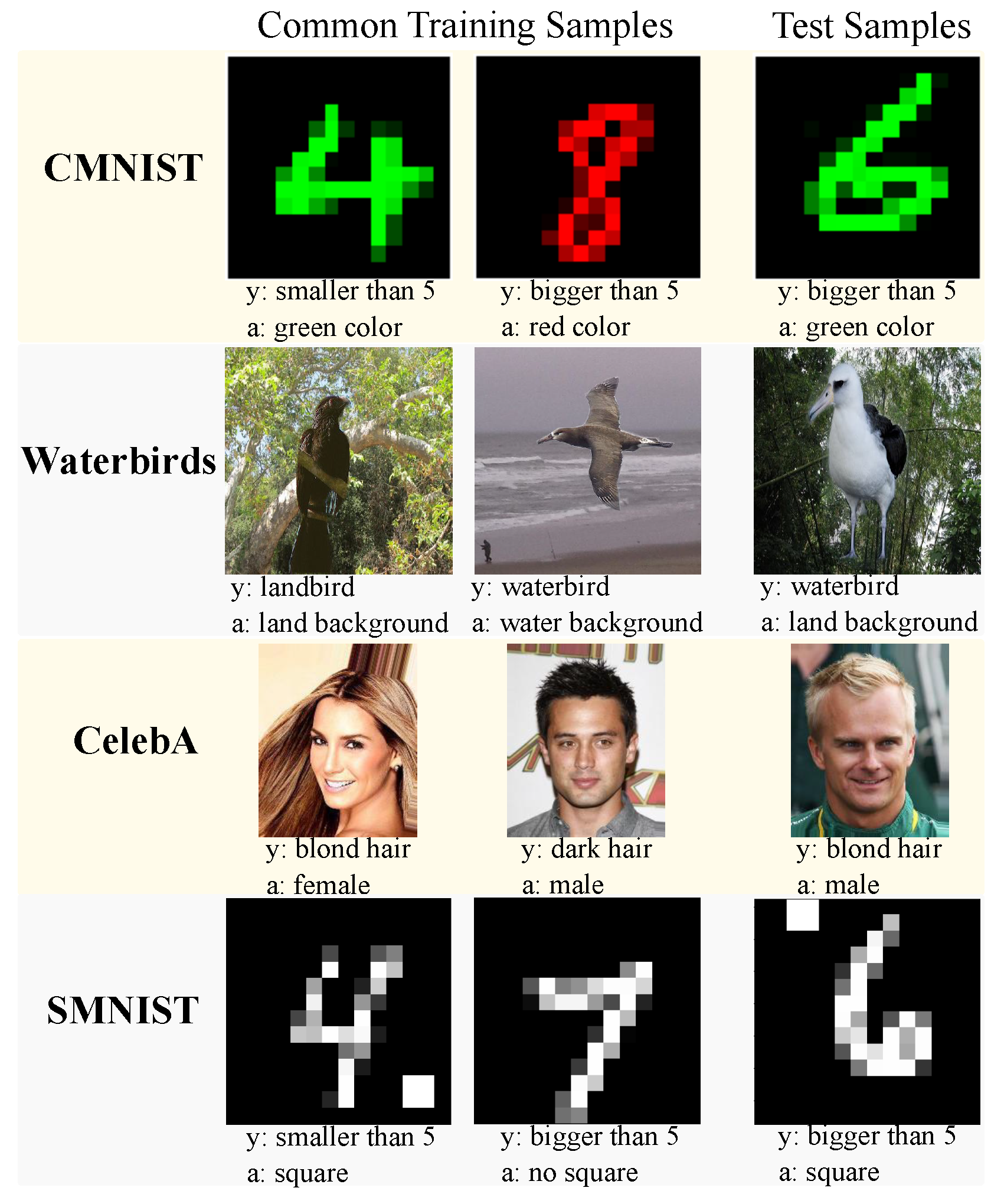
- We introduce the Square-MNIST dataset to evaluate the ability of our model in more challenging scenarios where the true causal features (strokes) and spurious features (squares) closely resemble each other. Our evaluation demonstrates the superior performance of FEED compared to other environment discovery approaches.
2. Related Works
3. Frustratingly Easy Environment Discovery
| Algorithm 1 FEED Algorithm |
| Input: dataset , model M |
| Output: environments , |
| 1: Randomly initialize and using |
| 2: for epochs do |
| 3: train M by minimizing |
| 4: for do |
| 5: if then |
| 6: Assign to |
| 7: else |
| 8: Assign to |
| 9: end if |
| 10: end for |
| 11: end for |
| 12: return , |
4. Experiments
4.1. Dataset
4.2. Implementation Details
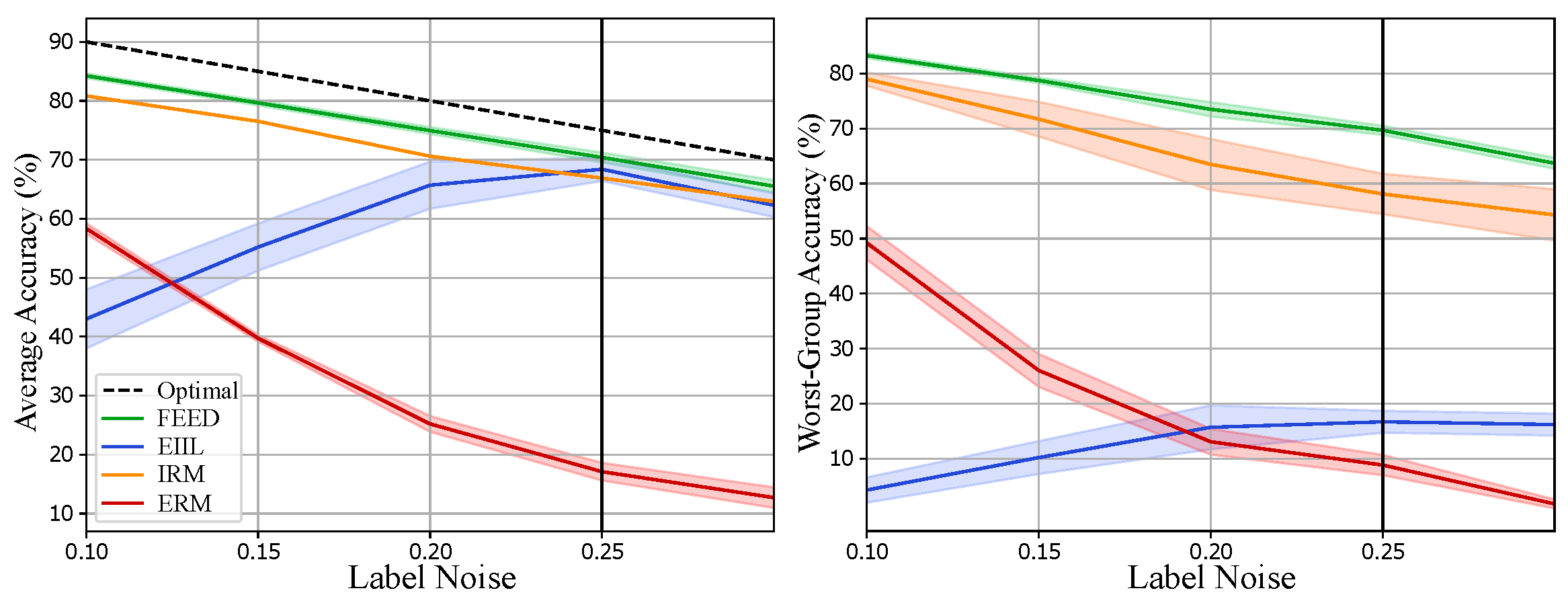
4.3. Results and Discussions
5. Conclusions
Author Contributions
Funding
Institutional Review Board Statement
Informed Consent Statement
Data Availability Statement
Conflicts of Interest
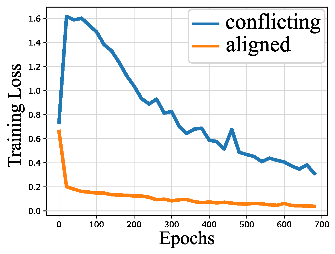
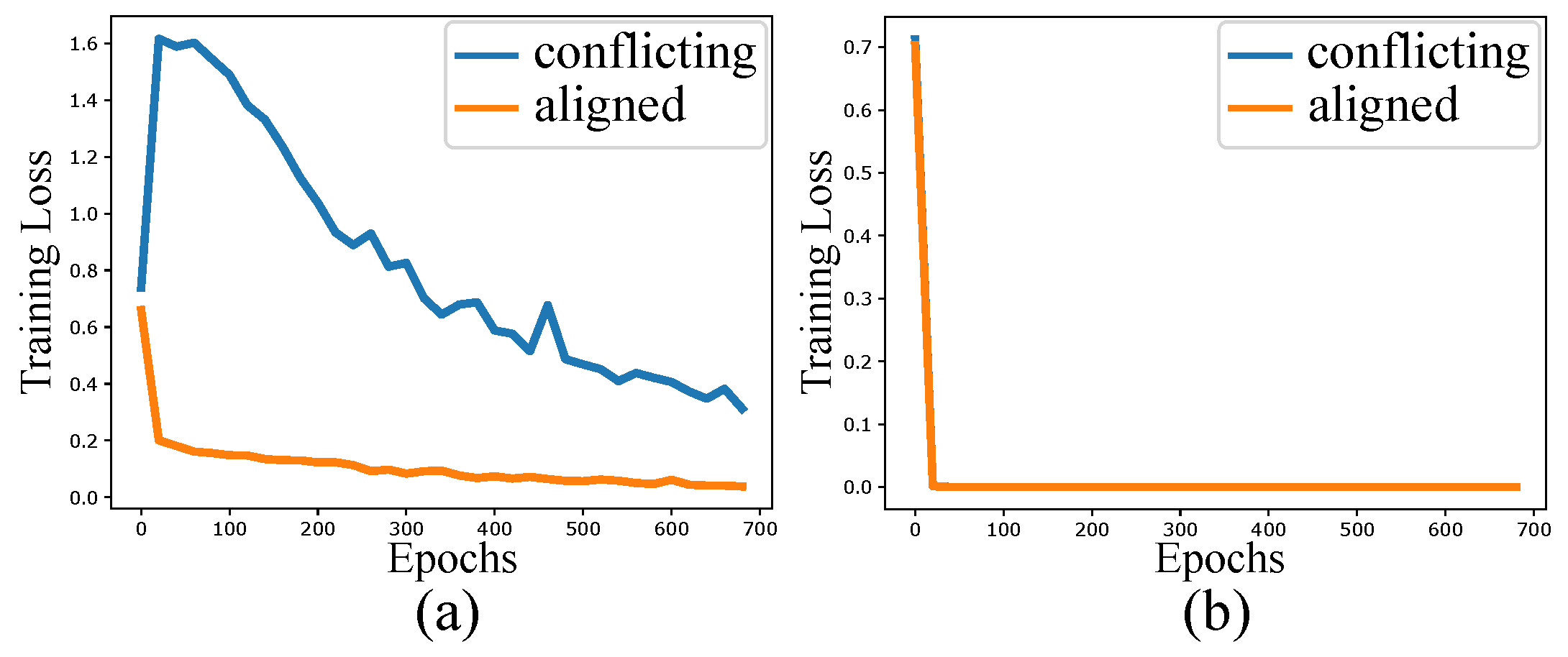
Appendix A. Loss Dynamics for CMNIST
Appendix B. Using Accuracy as Difficulty Score
Appendix C. Group Sufficiency Gap

| Standard CMNIST | CMNIST FEED | CMNIST EIIL | SMNIST FEED | SMNIST EIIL | ||||||
|---|---|---|---|---|---|---|---|---|---|---|
| 90.0 | 80.0 | 100.0 | 0.0 | 93.0 | 7.0 | 99.93 | 4.95 | 85.16 | 9.68 | |
| 10.0 | 20.0 | 0.0 | 100.0 | 7.0 | 93.0 | 0.07 | 95.05 | 14.84 | 90.32 | |
| 10.0 | 20.0 | 0.0 | 100.0 | 6.0 | 89.0 | 0.31 | 98.64 | 15.15 | 89.63 | |
| 90.0 | 80.0 | 100.0 | 0.0 | 94.0 | 11.0 | 99.69 | 1.36 | 84.85 | 10.37 | |
References
- Geirhos, R.; Jacobsen, J.H.; Michaelis, C.; Zemel, R.; Brendel, W.; Bethge, M.; Wichmann, F.A. Shortcut learning in deep neural networks. Nat. Mach. Intell. 2020, 2, 665–673. [Google Scholar] [CrossRef]
- Mehrabi, N.; Morstatter, F.; Saxena, N.; Lerman, K.; Galstyan, A. A survey on bias and fairness in machine learning. ACM Comput. Surv. (CSUR) 2021, 54, 1–35. [Google Scholar] [CrossRef]
- Arjovsky, M.; Bottou, L.; Gulrajani, I.; Lopez-Paz, D. Invariant risk minimization. arXiv 2019, arXiv:1907.02893. [Google Scholar]
- Arpit, D.; Jastrzębski, S.; Ballas, N.; Krueger, D.; Bengio, E.; Kanwal, M.S.; Maharaj, T.; Fischer, A.; Courville, A.; Bengio, Y.; et al. A closer look at memorization in deep networks. In Proceedings of the International Conference on Machine Learning, PMLR, Sydney, NSW, Australia, 6–11 August 2017; pp. 233–242. [Google Scholar]
- Sagawa, S.; Koh, P.W.; Hashimoto, T.B.; Liang, P. Distributionally robust neural networks for group shifts: On the importance of regularization for worst-case generalization. arXiv 2019, arXiv:1911.08731. [Google Scholar]
- Creager, E.; Jacobsen, J.H.; Zemel, R. Environment inference for invariant learning. In Proceedings of the International Conference on Machine Learning, PMLR, Virtual Event, 18–24 July 2021; pp. 2189–2200. [Google Scholar]
- Liu, E.Z.; Haghgoo, B.; Chen, A.S.; Raghunathan, A.; Koh, P.W.; Sagawa, S.; Liang, P.; Finn, C. Just train twice: Improving group robustness without training group information. In Proceedings of the International Conference on Machine Learning, PMLR, Virtual Event, 18–24 July 2021; pp. 6781–6792. [Google Scholar]
- Howard, F.M.; Dolezal, J.; Kochanny, S.; Schulte, J.; Chen, H.; Heij, L.; Huo, D.; Nanda, R.; Olopade, O.I.; Kather, J.N.; et al. The impact of site-specific digital histology signatures on deep learning model accuracy and bias. Nat. Commun. 2021, 12, 1–13. [Google Scholar] [CrossRef] [PubMed]
- Larrazabal, A.J.; Nieto, N.; Peterson, V.; Milone, D.H.; Ferrante, E. Gender imbalance in medical imaging datasets produces biased classifiers for computer-aided diagnosis. Proc. Natl. Acad. Sci. USA 2020, 117, 12592–12594. [Google Scholar] [CrossRef] [PubMed]
- Oakden-Rayner, L.; Dunnmon, J.; Carneiro, G.; Ré, C. Hidden stratification causes clinically meaningful failures in machine learning for medical imaging. In Proceedings of the ACM Conference on Health, Inference, and Learning, Toronto, ON, Canada, 2–4 April 2020; pp. 151–159. [Google Scholar]
- Buolamwini, J.; Gebru, T. Gender shades: Intersectional accuracy disparities in commercial gender classification. In Proceedings of the Conference on Fairness, Accountability and Transparency, PMLR, New York, NY, USA, 23–24 February 2018; pp. 77–91. [Google Scholar]
- Krco, N.; Laugel, T.; Loubes, J.M.; Detyniecki, M. When Mitigating Bias is Unfair: A Comprehensive Study on the Impact of Bias Mitigation Algorithms. arXiv 2023, arXiv:2302.07185. [Google Scholar]
- Nam, J.; Cha, H.; Ahn, S.; Lee, J.; Shin, J. Learning from failure: De-biasing classifier from biased classifier. Adv. Neural Inf. Process. Syst. 2020, 33, 20673–20684. [Google Scholar]
- Krasanakis, E.; Spyromitros-Xioufis, E.; Papadopoulos, S.; Kompatsiaris, Y. Adaptive sensitive reweighting to mitigate bias in fairness-aware classification. In Proceedings of the 2018 World Wide Web Conference, Lyon, France, 23–27 April 2018; pp. 853–862. [Google Scholar]
- Tzeng, E.; Hoffman, J.; Saenko, K.; Darrell, T. Adversarial discriminative domain adaptation. In Proceedings of the IEEE Conference on Computer Vision and Pattern Recognition, Honolulu, HI, USA, 21–26 July 2017; pp. 7167–7176. [Google Scholar]
- Long, M.; Cao, Z.; Wang, J.; Jordan, M.I. Conditional adversarial domain adaptation. Adv. Neural Inf. Process. Syst. 2018, 31, 1647–1657. [Google Scholar]
- Krueger, D.; Caballero, E.; Jacobsen, J.H.; Zhang, A.; Binas, J.; Zhang, D.; Le Priol, R.; Courville, A. Out-of-distribution generalization via risk extrapolation (rex). In Proceedings of the International Conference on Machine Learning, PMLR, Virtual Event, 18–24 July 2021; pp. 5815–5826. [Google Scholar]
- Srivastava, M.; Hashimoto, T.; Liang, P. Robustness to spurious correlations via human annotations. In Proceedings of the International Conference on Machine Learning, PMLR, Virtual Event, 13–18 July 2020; pp. 9109–9119. [Google Scholar]
- Dagaev, N.; Roads, B.D.; Luo, X.; Barry, D.N.; Patil, K.R.; Love, B.C. A too-good-to-be-true prior to reduce shortcut reliance. arXiv 2021, arXiv:2102.06406. [Google Scholar] [CrossRef]
- Rosenfeld, E.; Ravikumar, P.; Risteski, A. Domain-adjusted regression or: Erm may already learn features sufficient for out-of-distribution generalization. arXiv 2022, arXiv:2202.06856. [Google Scholar]
- Idrissi, B.Y.; Arjovsky, M.; Pezeshki, M.; Lopez-Paz, D. Simple data balancing achieves competitive worst-group-accuracy. In Proceedings of the Conference on Causal Learning and Reasoning, PMLR, Eureka, CA, USA, 11–13 April 2022; pp. 336–351. [Google Scholar]
- Kirichenko, P.; Izmailov, P.; Wilson, A.G. Last layer re-training is sufficient for robustness to spurious correlations. arXiv 2022, arXiv:2204.02937. [Google Scholar]
- Bao, Y.; Chang, S.; Barzilay, R. Predict then interpolate: A simple algorithm to learn stable classifiers. In Proceedings of the International Conference on Machine Learning, PMLR, Virtual Event, 18–24 July 2021; pp. 640–650. [Google Scholar]
- Sohoni, N.; Dunnmon, J.; Angus, G.; Gu, A.; Ré, C. No subclass left behind: Fine-grained robustness in coarse-grained classification problems. Adv. Neural Inf. Process. Syst. 2020, 33, 19339–19352. [Google Scholar]
- Zhang, J.; Lopez-Paz, D.; Bottou, L. Rich feature construction for the optimization-generalization dilemma. In Proceedings of the International Conference on Machine Learning, PMLR, Baltimore, MD, USA, 17–23 July 2022; pp. 26397–26411. [Google Scholar]
- Lahoti, P.; Beutel, A.; Chen, J.; Lee, K.; Prost, F.; Thain, N.; Wang, X.; Chi, E. Fairness without demographics through adversarially reweighted learning. Adv. Neural Inf. Process. Syst. 2020, 33, 728–740. [Google Scholar]
- Yong, L.; Zhu, S.; Tan, L.; Cui, P. ZIN: When and How to Learn Invariance Without Environment Partition? Adv. Neural Inf. Process. Syst. 2022, 35, 24529–24542. [Google Scholar]
- Liu, J.; Hu, Z.; Cui, P.; Li, B.; Shen, Z. Heterogeneous risk minimization. In Proceedings of the International Conference on Machine Learning, PMLR, Virtual Event, 18–24 July 2021; pp. 6804–6814. [Google Scholar]
- Matsuura, T.; Harada, T. Domain generalization using a mixture of multiple latent domains. In Proceedings of the AAAI Conference on Artificial Intelligence, New York, NY, USA, 7–12 February 2020; Volume 34, pp. 11749–11756. [Google Scholar]
- Bae, J.H.; Choi, I.; Lee, M. Meta-learned invariant risk minimization. arXiv 2021, arXiv:2103.12947. [Google Scholar]
- Lin, Y.; Dong, H.; Wang, H.; Zhang, T. Bayesian invariant risk minimization. In Proceedings of the IEEE/CVF Conference on Computer Vision and Pattern Recognition, New Orleans, LA, USA, 18–24 June 2022; pp. 16021–16030. [Google Scholar]
- Wald, Y.; Feder, A.; Greenfeld, D.; Shalit, U. On calibration and out-of-domain generalization. Adv. Neural Inf. Process. Syst. 2021, 34, 2215–2227. [Google Scholar]
- Lin, Y.; Zhu, S.; Cui, P. ZIN: When and How to Learn Invariance by Environment Inference? arXiv 2022, arXiv:2203.05818. [Google Scholar]
- Yao, H.; Wang, Y.; Li, S.; Zhang, L.; Liang, W.; Zou, J.; Finn, C. Improving out-of-distribution robustness via selective augmentation. In Proceedings of the International Conference on Machine Learning, PMLR, Baltimore, MD, USA, 17–23 July 2022; pp. 25407–25437. [Google Scholar]
- Shi, Y.; Seely, J.; Torr, P.H.; Siddharth, N.; Hannun, A.; Usunier, N.; Synnaeve, G. Gradient matching for domain generalization. arXiv 2021, arXiv:2104.09937. [Google Scholar]
- Koyama, M.; Yamaguchi, S. Out-of-distribution generalization with maximal invariant predictor. arXiv 2020, arXiv:2008.01883. [Google Scholar]
- Rame, A.; Dancette, C.; Cord, M. Fishr: Invariant gradient variances for out-of-distribution generalization. In Proceedings of the International Conference on Machine Learning, PMLR, Baltimore, MD, USA, 17–23 July 2022; pp. 18347–18377. [Google Scholar]
- Sagawa, S.; Raghunathan, A.; Koh, P.W.; Liang, P. An investigation of why overparameterization exacerbates spurious correlations. In Proceedings of the International Conference on Machine Learning, PMLR, Virtual Event, 13–18 July 2020; pp. 8346–8356. [Google Scholar]
- Zhang, J.; Menon, A.; Veit, A.; Bhojanapalli, S.; Kumar, S.; Sra, S. Coping with label shift via distributionally robust optimisation. arXiv 2020, arXiv:2010.12230. [Google Scholar]
- Ben-Tal, A.; El Ghaoui, L.; Nemirovski, A. Robust Optimization; Princeton University Press: Princeton, NJ, USA, 2009; Volume 28. [Google Scholar]
- Ganin, Y.; Lempitsky, V. Unsupervised domain adaptation by backpropagation. In Proceedings of the International Conference on Machine Learning, PMLR, Lille, France, 7–9 July 2015; pp. 1180–1189. [Google Scholar]
- Zhao, H.; Des Combes, R.T.; Zhang, K.; Gordon, G. On learning invariant representations for domain adaptation. In Proceedings of the International Conference on Machine Learning, PMLR, Long Beach, CA, USA, 9–15 June 2019; pp. 7523–7532. [Google Scholar]
- Pezeshki, M.; Kaba, O.; Bengio, Y.; Courville, A.C.; Precup, D.; Lajoie, G. Gradient starvation: A learning proclivity in neural networks. Adv. Neural Inf. Process. Syst. 2021, 34, 1256–1272. [Google Scholar]
- Zhang, Z.; Sabuncu, M. Generalized cross entropy loss for training deep neural networks with noisy labels. Adv. Neural Inf. Process. Syst. 2018, 31, 8792–8802. [Google Scholar]
- Rockafellar, R.T.; Uryasev, S. Optimization of Conditional Value-at-Risk. J. Risk 2000, 2, 21–42. [Google Scholar] [CrossRef]
- Sun, B.; Saenko, K. Deep coral: Correlation alignment for deep domain adaptation. In Proceedings of the Computer Vision—ECCV 2016 Workshops, Amsterdam, The Netherlands, 8–10 and 15–16 October 2016; Proceedings, Part III 14. pp. 443–450. [Google Scholar]

| CMNIST | WaterBirds | CelebA | ||||
|---|---|---|---|---|---|---|
| Avg. Acc. | Worst-Group Acc. | Avg. Acc. | Worst-Group Acc. | Avg. Acc. | Worst-Group Acc. | |
| ERM | 17.1 ± 0.4% | 8.9 ± 1.8% | 97.3 ± 0.2% | 60.3 ± 1.9% | 95.6 ± 0.2% | 47.2 ± 3.7% |
| LfF | 42.7 ± 0.5% | 33.2 ± 2.2% | 91.2 ± 0.7% | 78.0 ± 2.3% | 85.1 ± 0.4% | 72.2 ± 1.4% |
| JTT | 16.3 ± 0.8% | 12.5 ± 2.4% | 93.3 ± 0.7% | 86.7 ± 1.2% | 88.0 ± 0.3% | 81.1 ± 1.7% |
| GEORGE | 12.8 ± 2.0% | 9.2 ± 3.6% | 95.7 ± 0.5% | 76.2 ± 2.0% | 94.6 ± 0.2% | 54.9 ± 1.9% |
| CVar DRO | 33.2 ± 0.5% | 27.9 ± 1.1% | 96.0 ± 1.0% | 75.9 ± 2.2% | 82.5 ± 0.6% | 64.4 ± 2.9% |
| Fish | 46.9 ± 0.9% | 35.6 ± 1.5% | 85.6 ± 0.8% | 64.0 ± 1.7% | 93.1 ± 0.4% | 61.2 ± 1.8% |
| SD | 68.4 ± 1.1% | 62.3 ± 1.4% | 76.8 ± 1.3% | 71.8 ± 1.8% | 91.6 ± 1.3% | 83.2 ± 2.0% |
| CORAL | 65.1 ± 2.5% | 60.2 ± 4.1% | 90.3 ± 1.1% | 79.8 ± 2.5% | 93.8 ± 0.9% | 76.9 ± 3.6% |
| IRM | 66.9 ± 1.1% | 58.1 ± 3.7% | – | – | – | – |
| vREx | 68.7 ± 0.7% | 63.8 ± 2.8% | – | – | – | – |
| EIIL+IRM | 68.4 ± 0.8% | 16.7 ± 14.2% | 90.3 ± 0.2% | 63.1 ± 1.0% | 72.5 ± 0.1% | 54.0 ± 0.8% |
| EIIL+vREx | 57.4 ± 0.8% | 14.7 ± 11.8% | 89.7 ± 0.8% | 65.2 ± 3.4% | 76.4 ± 0.7% | 54.9 ± 2.6% |
| EIIL+GroupDRO | 44.4 ± 1.0% | 35.2 ± 8.2% | 96.9 ± 0.8% | 78.7 ± 1.0% | 90.7 ± 0.5% | 71.3 ± 0.9% |
| FEED+IRM (ours) | 70.4 ± 0.02% | 69.7 ± 0.8% | 92.3 ± 0.2% | 88.4 ± 0.9% | 86.0 ± 0.5% | 81.3 ± 1.4% |
| FEED+vREx (ours) | 71.1 ± 0.08% | 69.1 ± 1.2% | 93.3 ± 0.3% | 88.6 ± 1.0% | 86.9 ± 0.8% | 83.7 ± 1.4% |
| FEED+GroupDRO (ours) | 71.4 ± 0.02% | 71.0 ± 0.05% | 90.0 ± 0.3% | 88.0 ± 1.2% | 87.3 ± 0.6% | 84.3 ± 2.0% |
| GroupDRO | 71.4 ± 0.02% | 71.0 ± 0.05% | 93.5 ± 0.3% | 91.4 ± 1.1% | 92.9 ± 0.2% | 88.9 ± 2.3% |
| CMNIST | WaterBirds | CelebA | ||||
|---|---|---|---|---|---|---|
| 100.0 | 0.0 | 93.8 | 7.2 | 95.5 | 4.5 | |
| 0.0 | 100.0 | 16.9 | 83.1 | 99.5 | 0.5 | |
| 0.0 | 100.0 | 10.7 | 89.3 | 82.8 | 17.2 | |
| 100.0 | 0.0 | 81.5 | 18.5 | 30.5 | 69.5 | |
| Avg. Acc. | Worst-Group Acc. | |
|---|---|---|
| ERM | 72.1% | 68.1% |
| LfF | 34.5% | 13.3% |
| JTT | 26.1% | 18.1% |
| CVar DRO | 38.4% | 35.1% |
| SD | 79.1% | 74.9% |
| IRM | 78.3% | 75.3% |
| vREx | 83.5% | 81.7% |
| EIIL+IRM | 42.8% | 12.6% |
| EIIL+vREx | 42.5% | 6.0% |
| EIIL+GroupDRO | 12.9% | 2.5% |
| FEED+IRM (ours) | 85.6% | 84.7% |
| FEED+vREx (ours) | 85.9% | 85.2% |
| FEED+GroupDRO (ours) | 86.1% | 85.4% |
| GroupDRO | 86.1% | 85.4% |
| Avg. Acc. | Worst-Group Acc. | |
|---|---|---|
| ERM | 37.3% | 4.7% |
| LfF | 46.1% | 43.3% |
| JTT | 47.6% | 23.3% |
| CVar DRO | 49.0% | 40.1% |
| IRM | 41.6% | 5.8% |
| vREx | 54.7% | 12.2% |
| EIIL+IRM | 57.0% | 32.0% |
| EIIL+vREx | 58.9% | 38.2% |
| EIIL+GroupDRO | 67.6% | 57.0% |
| CE FEED+IRM | 36.8% | 3.7% |
| CE FEED+vREx | 33.7% | 3.2% |
| CE FEED+GroupDRO | 35.6% | 8.8% |
| FEED+IRM (ours) | 69.8% | 65.0% |
| FEED+vREx (ours) | 69.2% | 63.4% |
| FEED+GroupDRO (ours) | 71.3% | 65.0% |
| GroupDRO | 70.5% | 67.8% |
Disclaimer/Publisher’s Note: The statements, opinions and data contained in all publications are solely those of the individual author(s) and contributor(s) and not of MDPI and/or the editor(s). MDPI and/or the editor(s) disclaim responsibility for any injury to people or property resulting from any ideas, methods, instructions or products referred to in the content. |
© 2024 by the authors. Licensee MDPI, Basel, Switzerland. This article is an open access article distributed under the terms and conditions of the Creative Commons Attribution (CC BY) license (https://creativecommons.org/licenses/by/4.0/).
Share and Cite
Zare, S.; Nguyen, H.V. Frustratingly Easy Environment Discovery for Invariant Learning. Comput. Sci. Math. Forum 2024, 9, 2. https://doi.org/10.3390/cmsf2024009002
Zare S, Nguyen HV. Frustratingly Easy Environment Discovery for Invariant Learning. Computer Sciences & Mathematics Forum. 2024; 9(1):2. https://doi.org/10.3390/cmsf2024009002
Chicago/Turabian StyleZare, Samira, and Hien Van Nguyen. 2024. "Frustratingly Easy Environment Discovery for Invariant Learning" Computer Sciences & Mathematics Forum 9, no. 1: 2. https://doi.org/10.3390/cmsf2024009002
APA StyleZare, S., & Nguyen, H. V. (2024). Frustratingly Easy Environment Discovery for Invariant Learning. Computer Sciences & Mathematics Forum, 9(1), 2. https://doi.org/10.3390/cmsf2024009002