On Periodic Generalized Poisson INGARCH Models ^†

Abstract

This article discusses the class of Periodic Generalized Poisson Integer-Valued Generalized Autoregressive Conditional Heteroscedastic $\left(PGPINGARCH\right)$ models. The model, in addition to properly capture the periodic feature in the autocovariance structure, encompasses different types of dispersions, with this conditional marginal distribution. The main theoretical properties of this model are developed, in particular, the first two moment periodically stationary conditions, while the closed form of these moments are derived. Moreover, the existence of the higher order moment and their closed forms are established. The periodic autocovariance structure is studied. The estimation is done by the Yule Walker and the Conditional Maximum Likelihood methods and their performance is shown via an simulation study. Moreover, an application on Campylobacteriosis time series is provided, which indicates that the proposed models performs better than other models in the literature.

1. Introduction

Since the seminal paper by Ferland et al. [1] on modelling discrete-valued time series of counts via the integer-valued generalized autoregressive conditional Heteroscedastic $\left(INGARCH\right)$ model, there has been thereon several notable contributions in this field Zhu (2008) [2], Zhu (2009) [3], Fokianos et al. (2009) [4], Fokianos and Fried (2010) [5] and Doukhan et al. (2020) [6]. In particular, in Zhu (2011) [7] and Zhu (2012) [8,9,10], the $INGARCH$ time series models with different probability deviates that include Poisson, Negative-Binomial, Generalized Poisson, COM-Poisson and among other models have extensively explored. The general way of writing the $INGARCH$ model of order p and q is

$$\begin{array}{c}{X}_t\left|X_{t-1},X_{t-2,\dots }\right.⇝D\left({\mu }_t,{\eta }_t\right),\\ {\mu }_t={\alpha }_{0,t}+{\sum }_{i=1}^p{\alpha }_{i,t}{X}_{t-i}+{\sum }_{j=1}^q{\beta }_{j,t}{\mu }_{t-j},\end{array}$$

D is the probability model and ${\mu }_t$ and ${\eta }_t$ are the link or mean predictor functions and the dispersion parameter, respectively. Of course, the $INARCH$ process can be obtained as a special case. This approach of modelling the time series of counts can be viewed as a suitable alternative to the thinning-based integer-valued autoregressive process $\left(INAR\right)$ described in McKenzie (1986) [11], McKenzie (1988) [12], Al-Osh (1987) [13] and Weiß (2018) [14] and just to name some few. In fact, as argued by Zhu (2012) [8], the $INGARCH$ provides a better framework to model the discrete valued series as such class does not impose any innovation series distributions while ensures that the counting series follow the required distribution. As illustrated in Zhu (2012) [8], the $INGARCH$ yields better Akaike information criteria than the $INAR$ type processes. Due to these merits, the $INGARCH$ processes achieve a wider variety of application domains that comprise of series of varied levels of over- or under-dispersion.

To render the $INGARCH$ process more flexible, this paper proposes to explore the periodicity feature often observed in integer-valued time series applications, in the $INGARCH$ process and set up a new periodic $INGARCH$ type model. In the same direction, Bentarzi and Bentarzi (2017) [15] proposed a periodic Poisson $INGARCH$. However, the Poisson distribution is not usually suitable for modeling overdispersion and underdispersion time series. As a natural extension of the Poisson distribution, the Generalized Poisson distribution introduced by Consul and Jain (1973) [16], Consul (1989) [17], is quite flexible and allows for both overdispersion and underdispersion. On the other hand, as mentioned by Zhu (2012) [9], the Double Poisson distribution $\left(DP\right)$ introduced by Efron (1986) [18], which deal underdispersion phenomena is difficult to be used due to the fact that the $DP$ distribution does not well studied, thus many properties of the model are difficult to be established. However, for the overdispersion phenomena, the Negative Binomial distribution $\left(NB\right)$ is not usually suitable due to the integer valued first parameter, it follows that the joint maximum likelihood estimator $\left(MLE\right)$ of this parameter and other parameters, can be obtained.

In this sense, we propose a Periodic Generalized Poisson $INGARCH$ model, whose conditional distribution encompasses different dispersion. Moreover, the proposed periodic model reduces to the aperiodic $GPINGARCH$ model introduced by Zhu (2012) [9], while for the pure Poisson case, it reduces to the $PINGARCH$ introduced by Bentarzi and Bentarzi (2017) [15].

The rest of the paper is organized as follows: Section 2 provide the definition of the class of Periodic Generalized Poisson $INGARCH$ models. Section 3 presents the necessary and sufficient periodically stationary conditions. Furthermore, the closed-form expressions of the first two moments are obtained, under these conditions. The existence of higher moments and their calculations are considered in Section 4. Section 5 deals with the study of the autocovariance structure of the underlying model. Section 6 focuses on the estimation of the periodic unknown parameters using the Yule-Walker method $\left(YW\right)$ method and the Conditional Maximum Likelihood $\left(CML\right)$ method. In Section 7, the performance of the proposed estimation methods is shown via a simulation study and presents a comparative analysis in the context of monthly number of infections by Campylobacteriosis modeling with discussion of the model adequacy. Finally, some conclusions are shown in Section 8.

2. Notations, Definitions and Main Assumptions

A periodically correlated Integer-Valued process $\left\{X_t,t\in \mathbb{Z}\right\}$ in the sense of Gladyshev (1963) [19], with period S (where S $\ge 2$), is said to satisfy a Periodic Generalized Poisson Integer-Valued Generalized Autoregressive Conditional Heteroscedastic model, with orders p and q, noted $PGPINGARC{H}_S(p,q)$, if it the following form

$$\begin{array}{c}{X}_t\left|{\mathcal{F}}_{t-1}\right.⇝GP\left({\lambda }_t^{*},{\kappa }_t\right),\\ \frac{{\lambda }_t^{*}}{\left(1-{\kappa }_t\right)}={\lambda }_t={\alpha }_{0,t}+{\sum }_{i=1}^p{\alpha }_{i,t}{X}_{t-i}+{\sum }_{j=1}^q{\beta }_{j,t}{\lambda }_{t-j},\end{array}$$

(1)

where the parameters ${\alpha }_{0,t}>0$, ${\alpha }_{i,t}\ge 0$, ${\beta }_{j,t}\ge 0$, $i=1,\dots ,p$, $j=1,\dots ,q$ with $p\ge 1$, $q\ge 0$ and $max\left(-1,-{\lambda }_t^{*}/4\right)<{\kappa }_t<1$, are periodic in t with period S, i.e., ${\alpha }_{0,t+rS}={\alpha }_{0,t}$, ${\alpha }_{i,t+rS}={\alpha }_{i,t}$, ${\beta }_{j,t+rS}={\beta }_{j,t}$ and ${\kappa }_{t+rS}={\kappa }_t$, $\forall t,r\in \mathbb{Z}$. ${\mathcal{F}}_{t-1}$ denotes, as usually, the $\sigma$-field generated by $\left\{X_{t-1},X_{t-2},\dots \right\}$. Particularly, we have, for $p=q=1$, the periodic $GPINGARC{H}_S(1,1)$ model, which is the object in this paper:

$$\begin{array}{c}{X}_t\left|{\mathcal{F}}_{t-1}\right.⇝GP\left({\lambda }_t^{*},{\kappa }_t\right),\\ \frac{{\lambda }_t^{*}}{\left(1-{\kappa }_t\right)}={\lambda }_t={\alpha }_{0,t}+{\alpha }_{1,t}{X}_{t-1}+{\beta }_t{\lambda }_{t-1}.\end{array}$$

(2)

where the parameters ${\alpha }_{0,t}$, ${\alpha }_{1,t}$ and ${\beta }_t$ are periodic in t with period S, i.e., ${\alpha }_{0,t+rS}={\alpha }_{0,t}$, ${\alpha }_{1,t+rS}={\alpha }_{1,t}$, ${\beta }_{t+rS}={\beta }_t$ and ${\kappa }_{t+rS}={\kappa }_t$, $\forall t,r\in \mathbb{Z}$. Letting $t=s+\tau S$ for $s=1,2,\dots ,S$ and $\tau \in \mathbb{Z}$, the last model (2) can be rewritten in the equivalent form

$$\begin{array}{c}{X}_{s+\tau S}\left|{\mathcal{F}}_{s-1+\tau S}\right.⇝GP\left({\lambda }_{s+\tau S}^{*},{\kappa }_s\right),\\ \frac{{\lambda }_{s+\tau S}^{*}}{\left(1-{\kappa }_s\right)}={\lambda }_{s+\tau S}={\alpha }_{0,s}+{\alpha }_{1,s}{X}_{s-1+\tau S}+{\beta }_s{\lambda }_{s-1+\tau S}.\end{array}$$

(3)

Clearly, when $q=0$, the model (1) is denoted by $PGPINARC{H}_S\left(p\right)$. When ${\kappa }_t$, the above model reduces to Poisson $PINGARC{H}_S(1,1)$ studied by Bentarzi and Bentarzi (2017) [15]. This model extends the following time-invariant (i.e., $S=1$) $GPINGARCH(1,1)$ studied by Zhu (2012) [9] to the time periodic case,

$$\begin{array}{c}{X}_t\left|{\mathcal{F}}_{t-1}\right.⇝GP\left({\lambda }_t^{*},\kappa \right),\\ \frac{{\lambda }_t^{*}}{\left(1-\kappa \right)}={\lambda }_t={\alpha }_0+{\alpha }_1{X}_{t-1}+\beta {\lambda }_{t-1}.\end{array}$$

(4)

3. Periodically Stationary Conditions

This section is devoted to establish the periodic stationarity conditions on the parameters of the $GPINGARC{H}_S(1,1)$ model (2), with respect to the first two order moments. Furthermore, under these conditions, the closed forms of the unconditional mean and the unconditional variance are obtained.

3.1. Periodically Stationary in the Mean

Proposition 1. 

The periodically correlated integer-valued process $\left\{X_t,t\in \mathbb{Z}\right\}$, satisfying the periodic $GPINGARC{H}_S(1,1)$ model (2), is periodically stationary, in the mean, if and only if,

$${\Pi }_{i=1}^S\left({\alpha }_{1,i}+{\beta }_i\right)<1.$$

(5)

Furthermore, the closed-form of the mean ${\mu }_{X,s}=\mathbb{E}\left(X_s\right),s=1,\dots ,S,$ of such process is, under this condition, given by:

$${\mu }_{X,s}={\left[I-{\Pi }_{i=1}^S\left({\alpha }_{1,i}+{\beta }_i\right)\right]}^{-1}{\sum }_{j=1}^S\left[{\Pi }_{i=1}^{j-1}\left({\alpha }_{1,s-i+1}+{\beta }_{s-i+1}\right)\right]{\alpha }_{0,s-j+1},$$

(6)

with the convention ${\Pi }_{i=1}^j{x}_i=1$ if $j<1$.

In the particular case of periodic $GPINARC{H}_S\left(1\right)$ model (4), i.e., $\left(q=0\right)$, the results of this proposition can be presented by the following corollary.

Corollary 1. 

The periodically correlated process $\left\{X_t,t\in \mathbb{Z}\right\}$ satisfying the periodic $GPINARC{H}_S\left(1\right)$ model, is periodically stationary in the mean if and only if

$${\Pi }_{i=1}^S{\alpha }_{1,i}<1.$$

(7)

Furthermore, the closed-form of the mean ${\mu }_{X,s},s=1,\dots ,S$, is then given by:

$${\mu }_{X,s}={\left[I-{\Pi }_{i=1}^S{\alpha }_{1,i}\right]}^{-1}{\sum }_{j=1}^{\mathbb{S}}\left[{\Pi }_{i=1}^{j-1}{\Pi }_{i=1}^S{\alpha }_{1,i}\right]{\alpha }_{0,s-j+1},$$

(8)

Proof of Proposition 1. 

The unconditional mean of the periodically correlated process $\left\{X_t,t\in \mathbb{Z}\right\}$, satisfying a $GPINGARC{H}_S(1,1)$ model (2) is given by

$${\mu }_{X,s}=\mathbb{E}\left(X_t\right)=\mathbb{E}\left(\mathbb{E}\left(X_t\left|{\mathcal{F}}_{t-1}\right.\right)\right)=\mathbb{E}\left({\lambda }_t\right)$$

where

$$\begin{array}{ccc}\hfill \mathbb{E}\left(X_t\right)& =& {\alpha }_{0,t}+{\alpha }_{1,t}\mathbb{E}\left(X_{t-1}\right)+{\beta }_t\mathbb{E}\left({\lambda }_{t-1}\right)\hfill \\ & =& {\psi }_{1,t}\mathbb{E}\left(X_{t-1}\right)+{\alpha }_{0,t}\hfill \end{array}$$

where ${\psi }_{1,t}=\left({\alpha }_{1,t}+{\beta }_t\right)$. Substituting successively, m times, in the last equation, we obtain,

$${\mu }_{X,t}=\left({\Pi }_{i=1}^m{\psi }_{1,t-i+1}\right){\mu }_{X,t-m}+{\sum }_{j=1}^m\left({\Pi }_{i=1}^{j-1}{\psi }_{1,t-i+1}\right){\alpha }_{0,t-j+1}.$$

Replacing m by t and letting $t=s+\tau S$, $s=1,2,\dots ,S$ and $\tau \in \mathbb{Z}$, while taking account of the periodicity of the parameters, one can obtain

$$\begin{array}{ccc}\hfill {\mu }_{X,s+\tau S}& =& \left({\Pi }_{i=1}^{s+\tau S}{\psi }_{1,s-i+1}\right){\mu }_{X,s+\tau S-s+\tau S}+{\sum }_{j=1}^{s+\tau S}\left({\Pi }_{i=1}^{j-1}{\psi }_{1,s-i+1}\right){\alpha }_{0,s-j+1},\hfill \\ & =& \left({\Pi }_{i=1}^{s+\tau S}{\psi }_{1,s-i+1}\right){\mu }_{X,0}+{\sum }_{j=1}^{s+\tau S}\left({\Pi }_{i=1}^{j-1}{\psi }_{1,s-i+1}\right){\alpha }_{0,s-j+1},\hfill \\ & =& {\left({\Pi }_{i=1}^S{\psi }_{1,i}\right)}^{\tau }\left({\Pi }_{i=1}^s{\psi }_{1,s-i+1}\right){\mu }_{X,0}+{\sum }_{j=1}^{\tau S}\left({\Pi }_{i=1}^{j-1}{\psi }_{1,s-i+1}\right){\alpha }_{0,s-j+1}\hfill \\ & & +{\sum }_{j=1}^s\left({\Pi }_{i=1}^{j-1+\tau S}{\psi }_{1,s-i+1}\right){\alpha }_{0,s-j+1},\hfill \\ & =& {\left({\Pi }_{i=1}^S{\psi }_{1,i}\right)}^{\tau }\left({\Pi }_{i=1}^s{\psi }_{1,s-i+1}\right){\mu }_{X,0}+{\sum }_{k=0}^{\tau -1}{\left({\Pi }_{i=1}^S{\psi }_{1,i}\right)}^k{\sum }_{j=1}^S\left({\Pi }_{i=1}^{j-1}{\psi }_{1,s-i+1}\right){\alpha }_{0,s-j+1}\hfill \\ & & +{\left({\Pi }_{i=1}^S{\psi }_{1,i}\right)}^{\tau }{\sum }_{j=1}^s\left({\Pi }_{i=1}^{j-1}{\psi }_{1,s-i+1}\right){\alpha }_{0,s-j+1},\hfill \\ & =& {\left({\Pi }_{i=1}^S{\psi }_{1,i}\right)}^{\tau }\left[\left({\Pi }_{i=1}^s{\psi }_{1,s-i+1}\right){\mu }_{X,0}+{\sum }_{j=1}^s\left({\Pi }_{i=1}^{j-1}{\psi }_{1,s-i+1}\right){\alpha }_{0,s-j+1}\right]\hfill \\ & & +{\left(1-{\Pi }_{i=1}^S{\psi }_{1,i}\right)}^{-1}\left[1-{\left({\Pi }_{i=1}^S{\psi }_{1,i}\right)}^{\tau }\right]{\sum }_{j=1}^S\left({\Pi }_{i=1}^j{\psi }_{1,s-i+1}\right){\alpha }_{0,s-j+1}.\hfill \end{array}$$

Letting $t\to \infty$, i.e., $\tau \to \infty$, then ${\mu }_{X,s}$ for $s=1,\dots ,S$ converge to

$${\left(1-{\Pi }_{i=1}^S{\psi }_{1,i}\right)}^{-1}{\sum }_{j=1}^S\left({\Pi }_{i=1}^j{\psi }_{1,s-i+1}\right){\alpha }_{0,s-j+1},$$

if and only if ${\Pi }_{i=1}^S{\psi }_{1,i}<1.$ □

3.2. Periodically Stationary in the Second Order

Proposition 2. 

The integer-valued periodically stationary in the mean process $\left\{X_t,t\in \mathbb{Z}\right\}$, satisfying the periodic $GPINGARC{H}_S(1,1)$ model (2), is periodically stationary in the second order, if and only if,

$${\Pi }_{i=1}^S{\left({\alpha }_{1,i}+{\beta }_i\right)}^2<1.$$

(9)

Furthermore, the closed-form of the variances ${\gamma }_X^{\left(s\right)}\left(0\right)$ of such process and ${\gamma }_{\lambda }^{\left(s\right)}\left(0\right),s=1,\dots ,S$, are, under this condition, given respectively by:

$$\begin{array}{ccc}\hfill {\gamma }_X^{\left(s\right)}\left(0\right)& =& {\phi }_s^2{\mu }_{X,s}+{\left(1-{\Pi }_{i=1}^S{\psi }_{2,i}\right)}^{-1}{\sum }_{j=1}^S\left({\Pi }_{i=1}^j{\psi }_{2,s-i+1}\right)F_{s-j+1},\hfill \end{array}$$

(10)

$$\begin{array}{ccc}\hfill {\gamma }_{\lambda }^{\left(s\right)}\left(0\right)& =& {\left(1-{\Pi }_{i=1}^S{\psi }_{2,i}\right)}^{-1}{\sum }_{j=1}^S\left({\Pi }_{i=1}^j{\psi }_{2,s-i+1}\right){\Lambda }_{s-j+1},\hfill \end{array}$$

(11)

where ${\psi }_{2,t}={\left({\alpha }_{1,t}+{\beta }_t\right)}^2$, ${\phi }_s={\left(1-{\kappa }_s\right)}^{-1}$ and $F_s={\alpha }_{1,s}^2{\phi }_{s-1}^2{\mu }_{\lambda ,s-1}$, with the convention ${\Pi }_{i=1}^j{x}_i=1$ if $j<1$.

The following corollary, gives the periodic stationarity in second order for the particular case of periodic $GPINARC{H}_S\left(1\right)$ model (4).

Corollary 2. 

The periodically correlated integer-valued process $\left\{X_t,t\in \mathbb{Z}\right\}$ stationary in the mean, satisfying the periodic $GPINARC{H}_S\left(1\right)$ model (4), is periodically stationary in the second order, if and only if,

$${\Pi }_{i=1}^S{\alpha }_{1,i}^2<1.$$

(12)

Furthermore, the closed-form of the variances ${\gamma }_X^{\left(s\right)}\left(0\right)$ of such process and ${\gamma }_{\lambda }^{\left(s\right)}\left(0\right),s=1,\dots ,S$, are, under this condition, given, respectively, by:

$$\begin{array}{ccc}\hfill {\gamma }_X^{\left(s\right)}\left(0\right)& =& {\phi }_s^2{\mu }_{X,s}+{\left(1-{\Pi }_{i=1}^S{\alpha }_{1,s}^2\right)}^{-1}\left[1-{\left({\Pi }_{i=1}^S{\alpha }_{1,s}^2\right)}^{\tau }\right]{\sum }_{j=1}^S\left({\Pi }_{i=1}^j{\alpha }_{1,s-i+1}^2\right)F_{s-j+1},\hfill \end{array}$$

(13)

$$\begin{array}{ccc}\hfill {\gamma }_{\lambda }^{\left(s\right)}\left(0\right)& =& {\left(1-{\Pi }_{i=1}^S{\alpha }_{1,s}^2\right)}^{-1}\left[1-{\left({\Pi }_{i=1}^S{\alpha }_{1,s}^2\right)}^{\tau }\right]{\sum }_{j=1}^S\left({\Pi }_{i=1}^j{\alpha }_{1,s-i+1}^2\right)F_{s-j+1}.\hfill \end{array}$$

(14)

Proof of Proposition 2. 

The unconditional variance of the periodically correlated process $\left\{X_t,t\in \mathbb{Z}\right\}$, satisfying a $GPINGARC{H}_S(1,1)$ model (2) is given by

$$\begin{array}{ccc}\hfill Var\left(X_t\right)& =& Var\left(\mathbb{E}\left(X_t\left|{\mathcal{F}}_{t-1}\right.\right)\right)+\mathbb{E}\left(Var\left(X_t\left|{\mathcal{F}}_{t-1}\right.\right)\right),\hfill \\ & =& {\phi }_t^2\mathbb{E}\left({\lambda }_t\right)+Var\left({\lambda }_t\right),\hfill \end{array}$$

where ${\phi }_t={\left(1-{\kappa }_t\right)}^{-1}$. The last equation can be written in the following equivalent form

$${\gamma }_X^{\left(s\right)}\left(0\right)={\phi }_s^2{\mu }_{X,s}+{\gamma }_{\lambda }^{\left(s\right)}\left(0\right).$$

(15)

The mean ${\mu }_{X,s}$ was calculated previously and is given by (6), then we need to calculate ${\gamma }_{\lambda }^{\left(s\right)}\left(0\right)$, which is given as follows

$$\begin{array}{ccc}\hfill {\gamma }_{\lambda }^{\left(t\right)}\left(0\right)& =& Var\left({\alpha }_{0,t}+{\alpha }_{1,t}{X}_{t-1}+{\beta }_t{\lambda }_{t-1}\right),\hfill \\ & =& Var\left({\alpha }_{1,t}{X}_{t-1}\right)+Var\left({\beta }_t{\lambda }_{t-1}\right)+2Cov\left({\alpha }_{1,t}{X}_{t-1},{\beta }_t{\lambda }_{t-1}\right),\hfill \\ & =& {\alpha }_{1,t}^{2}Var\left(X_{t-1}\right)+{\beta }_t^{2}Var\left({\lambda }_{t-1}\right)+2{\alpha }_{1,t}{\beta }_{t}Var\left({\lambda }_{t-1}\right),\hfill \\ & =& {\left({\alpha }_{1,t}+{\beta }_t\right)}^2{\gamma }_{\lambda }^{\left(t-1\right)}\left(0\right)+{\alpha }_{1,t}^2{\phi }_{t-1}^2{\mu }_{\lambda ,t-1},\hfill \\ & =& {\psi }_{2,t}{\gamma }_{\lambda }^{\left(t-1\right)}\left(0\right)+F_t,\hfill \end{array}$$

where ${\psi }_{2,t}={\left({\alpha }_{1,t}+{\beta }_t\right)}^2$ and $F_t={\alpha }_{1,t}^2\phi$${}_{t-1}^2{\mu }_{\lambda ,t-1}$. By iterating m times, we obtain

$${\gamma }_{\lambda }^{\left(t\right)}\left(0\right)=\left({\Pi }_{i=1}^m{\psi }_{2,t-i+1}\right){\gamma }_{\lambda }^{\left(t-m\right)}\left(0\right)+{\sum }_{j=1}^m\left({\Pi }_{i=1}^{j-1}{\psi }_{2,t-i+1}\right)F_{t-j+1}.$$

Replacing m by t and letting $t=s+\tau S$, $s=1,2,\dots ,S$ and $\tau \in \mathbb{Z}$, while taking account of the periodicity of the parameters and following the same steps of Proof of Proposition 1, we obtain

$$\begin{array}{ccc}\hfill {\gamma }_{\lambda }^{\left(s+\tau S\right)}\left(0\right)& =& \left({\Pi }_{i=1}^{s+\tau S}{\psi }_{2,s-i+1}\right){\gamma }_{\lambda }^{\left(0\right)}\left(0\right)+{\sum }_{j=1}^{s+\tau S}\left({\Pi }_{i=1}^{j-1}{\psi }_{2,s-i+1}\right)F_{s-j+1},\hfill \\ & =& {\left({\Pi }_{i=1}^S{\psi }_{2,i}\right)}^{\tau }\left[\left({\Pi }_{i=1}^s{\psi }_{2,s-i+1}\right){\gamma }_{\lambda }^{\left(0\right)}\left(0\right)+{\sum }_{j=1}^s\left({\Pi }_{i=1}^{j-1}{\psi }_{2,s-i+1}\right)F_{s-j+1}\right]\hfill \\ & & +{\left(1-{\Pi }_{i=1}^S{\psi }_{2,i}\right)}^{-1}\left[1-{\left({\Pi }_{i=1}^S{\psi }_{2,i}\right)}^{\tau }\right]{\sum }_{j=1}^S\left({\Pi }_{i=1}^j{\psi }_{2,s-i+1}\right)F_{s-j+1}.\hfill \end{array}$$

Therefore, the last equation converge, as $\tau \to \infty$ to

$${\gamma }_{\lambda }^{\left(s\right)}\left(0\right)={\left(1-{\Pi }_{i=1}^S{\psi }_{2,i}\right)}^{-1}{\sum }_{j=1}^S\left({\Pi }_{i=1}^j{\psi }_{2,s-i+1}\right)F_{s-j+1},$$

if and only if ${\Pi }_{i=1}^S{\psi }_{2,i}<1$. Then, the variance ${\gamma }_X^{\left(s\right)}\left(0\right)$ is given by

$${\gamma }_X^{\left(s\right)}\left(0\right)={\phi }_s^2{\mu }_{X,s}+{\left(1-{\Pi }_{i=1}^S{\psi }_{2,i}\right)}^{-1}{\sum }_{j=1}^S\left({\Pi }_{i=1}^j{\psi }_{2,s-i+1}\right)F_{s-j+1},$$

where ${\psi }_{2,s}={\left({\alpha }_{1,s}+{\beta }_s\right)}^2$, $\phi$${}_s={\left(1-{\kappa }_s\right)}^{-1}$ and $F_s={\alpha }_{1,s}^2\phi$ ${}_{s-1}^2{\mu }_{\lambda ,s-1}$. □

4. Existence of Higher Moments and Their Calculations

In this section, we establish the existence condition of the m-th order moment, $\mathbb{E}\left(X_t^m\right)$, for a second order periodic $GPINGARC{H}_S(1,1)$ model, satisfying (2). Moreover, under this condition, the closed form of $\mathbb{E}\left(X_t^m\right)$ is obtained. To state this main result, we need to define the following three m–column vector, ${\underline{\mu }}_{X,t}^{\left(m\right)}={\left(\mathbb{E}\left(X_t^m\right),\mathbb{E}\left(X_t^{m-1}\right),\dots ,\mathbb{E}\left(X_t\right)\right)}^{\prime }$, ${\underline{\Lambda }}_t^{\left(m\right)}={\left({\lambda }_t^m,{\lambda }_t^{m-1},\dots ,{\lambda }_t\right)}^{\prime }$, ${\underline{\alpha }}_{0,t}^{\left(m\right)}={\left({\alpha }_{0,t}^m,{\alpha }_{0,t}^{m-1},\dots ,{\alpha }_{0,t}\right)}^{\prime }$, and the two squared $m\times m$ matrices, ${\Phi }_t^{\left(m\right)}$ and ${\Omega }_{m,t}$, whose elements are given, respectively, for $i,j=1,\dots ,m$, by

$${\Phi }_t^{\left(m\right)}=\left\{\begin{array}{cc}0\hfill & \mathrm{if}i>j\hfill \\ {\psi }_{m-i+1,t}\hfill & \mathrm{if}i=j\hfill \\ {\varphi }_{m-j+1,t}^{\left(m-i+1\right)}\hfill & \mathrm{if}i<j\hfill \end{array}\right.,{\Omega }_{m,t}=\left\{\begin{array}{cc}0\hfill & \mathrm{if}i>j\hfill \\ b_{\left(m-i+1\right)\left(m-i+1\right),t}\hfill & \mathrm{if}i=j\hfill \\ b_{\left(m-i+1\right)\left(m-j+1\right),t}\hfill & \mathrm{if}i<j\hfill \end{array}\right.$$

(16)

where,

$$\begin{array}{ccc}\hfill {\varphi }_{i,t}^{\left(m\right)}& =& \left(\genfrac{}{}{0pt}{}{m}{i}\right){\alpha }_{0,t}^{m-i}{\psi }_{i,t}+{\sum }_{j=i+1}^m{\sum }_{l=j-i}^{j-1}{\mathcal{K}}_{i,l+1,j-i,t}^{\left(m\right)}\hfill \end{array}$$

(17)

$$\begin{array}{ccc}\hfill {\mathcal{K}}_{i,j,l,t}^{\left(m\right)}& =& \left(\genfrac{}{}{0pt}{}{m}{i}\right)\left(\genfrac{}{}{0pt}{}{i}{j}\right){\alpha }_{0,t}^{m-i}{\alpha }_{1,t}^j{\beta }_t^{i-j}{b}_{j\left(j-l\right),t-1},\hfill \end{array}$$

(18)

$$\begin{array}{ccc}\hfill {\psi }_{i,t}& =& {\sum }_{j=0}^i\left(\genfrac{}{}{0pt}{}{i}{j}\right){\alpha }_{1,t}^j{\beta }_t^{i-j}{b}_{jj,t-1},\hfill \end{array}$$

(19)

where, according to Zhu (2012) [9], $b_{jl,t}$ is not related to ${\lambda }_t$, and $b_{jl,t}=1/{\left(1-{\kappa }_t\right)}^l$.

Proposition 3. 

The unconditional m-th moment, ${\mu }_{X,t}^{\left(m\right)}=\mathbb{E}\left(X_t^m\right)$, for the periodically correlated process $\left\{X_t,t\in \mathbb{Z}\right\}$ satisfying the periodic $GPINGARC{H}_S(1,1)$ model, exists and is finite, if and only if

$${\Pi }_{s=1}^S{\psi }_{m,s}<1,$$

(20)

where ${\psi }_{i,t}$ is given by (19). Furthermore, the closed form of the m-column vectors of the unconditional m-order moments, ${\underline{\mu }}_{X,t}^{\left(m\right)}$ and $\mathbb{E}\left({\underline{\Lambda }}_t^{\left(m\right)}\right)$ are given, under this condition, respectively, by

$$\begin{array}{ccc}\hfill \mathbb{E}\left({\underline{\Lambda }}_{s+\tau S}^{\left(m\right)}\right)& =& {\left(I-{\Pi }_{i=1}^S{\Phi }_{s-i+1}^{\left(m\right)}\right)}^{-1}{\sum }_{j=0}^{S-1}\left({\Pi }_{i=1}^{j-1}{\Phi }_{s-i+1}^{\left(m\right)}\right){\underline{\alpha }}_{0,s-j}^{\left(m\right)},\hfill \end{array}$$

(21)

$$\begin{array}{ccc}\hfill {\underline{\mu }}_{X,s}^{\left(m\right)}& =& {\Omega }_{m,s}{\left(I-{\Pi }_{i=1}^S{\Phi }_{s-i+1}^{\left(m\right)}\right)}^{-1}{\sum }_{j=0}^{S-1}\left({\Pi }_{i=1}^{j-1}{\Phi }_{s-i+1}^{\left(m\right)}\right){\underline{\alpha }}_{0,s-j}^{\left(m\right)}.\hfill \end{array}$$

(22)

where the elements of the matrices ${\Phi }_s^{\left(m\right)}$ and ${\Omega }_{m,s}$ are given by (16).

Proof of Proposition 3. 

The conditional m-th moment of ${\lambda }_t$, i.e., $\mathbb{E}\left({\lambda }_t^m\left|{\mathcal{F}}_{t-2}\right.\right)$ is given by

$$\mathbb{E}\left({\lambda }_t^m\left|{\mathcal{F}}_{t-2}\right.\right)={\sum }_{i=0}^m\left(\genfrac{}{}{0pt}{}{m}{i}\right){\alpha }_{0,t}^{m-i}{\sum }_{j=0}^i\left(\genfrac{}{}{0pt}{}{i}{j}\right){\alpha }_{1,t}^j{\beta }_t^{i-j}{\lambda }_{t-1}^{i-j}\mathbb{E}\left(X_{t-1}^j\left|{\mathcal{F}}_{t-2}\right.\right)$$

(23)

Using $\left(2.5\right)$ of Zhu (2012) [9], the j-th moment of a generalized Poisson random variable, is given by

$$\mathbb{E}\left(X_t^j\left|{\mathcal{F}}_{t-2}\right.\right)={\sum }_{l=1}^j{b}_{jl,t}{\lambda }_t^l,$$

(24)

where $b_{jl,t}$ is not related to ${\lambda }_t$, and $b_{jl,t}=1/{\left(1-{\kappa }_t\right)}^l$. Therefore,

$$\begin{array}{ccc}\hfill \mathbb{E}\left({\lambda }_t^m\left|{\mathcal{F}}_{t-2}\right.\right)& =& {\sum }_{i=0}^m\left(\genfrac{}{}{0pt}{}{m}{i}\right){\alpha }_{0,t}^{m-i}{\sum }_{j=0}^i\left(\genfrac{}{}{0pt}{}{i}{j}\right){\alpha }_{1,t}^j{\beta }_t^{i-j}{\lambda }_{t-1}^{i-j}{\sum }_{l=1}^j{b}_{jl,t-1}{\lambda }_{t-1}^l,\hfill \\ & =& {\alpha }_{0,t}^m+{\psi }_{m,t}{\lambda }_{t-1}^m+{\sum }_{i=1}^{m-1}{\sum }_{j=0}^i\left(\genfrac{}{}{0pt}{}{i}{j}\right){\alpha }_{0,t}^{m-i}{\alpha }_{1,t}^j{\beta }_t^{i-j}{b}_{jj,t-1}{\lambda }_{t-1}^i\hfill \\ & & +{\sum }_{i=1}^m{\sum }_{j=1}^i{\sum }_{l=1}^{j-1}\left(\genfrac{}{}{0pt}{}{m}{i}\right)\left(\genfrac{}{}{0pt}{}{i}{j}\right){\alpha }_{0,t}^{m-i}{\alpha }_{1,t}^j{\beta }_t^{i-j}{b}_{jl,t-1}{\lambda }_{t-1}^{i-j+l}.\hfill \end{array}$$

(25)

Using, the following notation,

$$\begin{array}{ccc}\hfill {\psi }_{i,t}& =& {\sum }_{j=0}^i\left(\genfrac{}{}{0pt}{}{i}{j}\right){\alpha }_{1,t}^j{\beta }_t^{i-j}{b}_{jj,t-1},\hfill \end{array}$$

(26)

$$\begin{array}{ccc}\hfill {\mathcal{K}}_{i,j,l,t}^{\left(m\right)}& =& \left(\genfrac{}{}{0pt}{}{m}{i}\right)\left(\genfrac{}{}{0pt}{}{i}{j}\right){\alpha }_{0,t}^{m-i}{\alpha }_{1,t}^j{\beta }_t^{i-j}{b}_{j\left(j-l\right),t-1}.\hfill \end{array}$$

(27)

The last equation, i.e., (25), can be rewritten in the following form

$$\mathbb{E}\left({\lambda }_t^m\left|{\mathcal{F}}_{t-2}\right.\right)={\alpha }_{0,t}^m+{\psi }_{m,t}{\lambda }_{t-1}^m+{\sum }_{i=1}^{m-1}\left(\genfrac{}{}{0pt}{}{m}{i}\right){\alpha }_{0,t}^{m-i}{\psi }_{i,t}{\lambda }_{t-1}^i+{\sum }_{i=1}^m{\sum }_{j=1}^i{\sum }_{l=1}^{j-1}{\mathcal{K}}_{i,j,l,t}^{\left(m\right)}{\lambda }_{t-1}^{i-l},$$

Therefore,

$$\mathbb{E}\left({\lambda }_t^m\left|{\Pi }_{t-2}\right.\right)={\alpha }_{0,t}^m+{\psi }_{m,t}{\lambda }_{t-1}^m+{\sum }_{i=1}^{m-1}{\varphi }_{i,t}^{\left(m\right)}{\lambda }_{t-1}^i,$$

(28)

where,

$${\varphi }_{i,t}^{\left(m\right)}=\left(\genfrac{}{}{0pt}{}{m}{i}\right){\alpha }_{0,t}^{m-i}{\psi }_{i,t}+{\sum }_{j=i+1}^m{\sum }_{l=j-i1}^{j-1}{\mathcal{K}}_{i,l+1,j-i,t}^{\left(m\right)}$$

in which ${\mathcal{K}}_{i,j,l,t}^{\left(m\right)}$ is given previously by (27). Replacing i in (28) by $m,m-1,\dots ,1$, we obtain the following equation

$$\mathbb{E}\left({\underline{\Lambda }}_t^{\left(m\right)}\left|{\Pi }_{t-2}\right.\right)={\Phi }_t^{\left(m\right)}{\underline{\Lambda }}_{t-1}^{\left(m\right)}+{\underline{\alpha }}_{0,t}^{\left(m\right)},$$

(29)

where the column vectors ${\underline{\Lambda }}_t^{\left(m\right)}$ and ${\underline{\alpha }}_{0,t}^{\left(m\right)}$ are given, respectively, by ${\left({\lambda }_t^m,{\lambda }_t^{m-1},\dots ,{\lambda }_t\right)}^{\prime }$ and ${\left({\alpha }_{0,t}^m,{\alpha }_{0,t}^{m-1},\dots ,{\alpha }_{0,t}\right)}^{\prime }$, while the $m\times m$ matrix ${\Phi }_t^{\left(m\right)}$ is given previously by (16).

Iterating Equation (29), n times, and letting $n=kS-2$, we obtain

$$\mathbb{E}\left({\underline{\Lambda }}_t^{\left(m\right)}\left|{\mathcal{F}}_{t-kS}\right.\right)=\left({\Pi }_{i=1}^{kS-1}{\Phi }_{t-i+1}^{\left(m\right)}\right){\underline{\Lambda }}_{t-\left(kS-1\right)}^{\left(m\right)}+{\sum }_{j=0}^{kS-2}\left({\Pi }_{i=1}^j{\Phi }_{t-i+1}^{\left(m\right)}\right){\underline{\alpha }}_{0,t-j}^{\left(m\right)}$$

Replacing t by $s+\tau S$$s=1,2,\dots ,S$ and $\tau \in \mathbb{Z}$, while taking account of the periodicity of the column vector ${\underline{\alpha }}_{0,t}^{\left(m\right)}$ and following the same steps of the Proof of Proposition 1, we obtain

$$\begin{array}{c}\mathbb{E}\left({\underline{\Lambda }}_{s+\tau S}^{\left(m\right)}\left|{\mathcal{F}}_{s-\left(\tau -k\right)S}\right.\right)={\left({\Pi }_{i=1}^S{\Phi }_{s-i+1}^{\left(m\right)}\right)}^{k-1}\left[{\sum }_{j=1}^{S-1}\left({\Pi }_{i=1}^{j-1}{\Phi }_{s-i+1}^{\left(m\right)}\right){\underline{\alpha }}_{0,s-j+1}^{\left(m\right)}+\left({\Pi }_{i=1}^{S-1}{\Phi }_{s-i+1}^{\left(m\right)}\right){\underline{\Lambda }}_{t-\left(\left\{k-\tau \right\}S-1\right)}^{\left(m\right)}\right]\\ +{\sum }_{l=0}^{k-2}{\left({\Pi }_{i=1}^S{\Phi }_{s-i+1}^{\left(m\right)}\right)}^l{\sum }_{j=1}^S\left({\Pi }_{i=1}^{j-1}{\Phi }_{s-i+1}^{\left(m\right)}\right){\underline{\alpha }}_{0,s-j+1}^{\left(m\right)}.\end{array}$$

The matrices ${\Phi }_{s-i+1}^{\left(m\right)}$ for $i=1,\dots ,S$ are diagonal with ${\psi }_{m,s-i+1},{\psi }_{m-1,s-i+1},\dots ,{\psi }_{1,s-i+1}$ as a eigenvalues, then a sufficient condition for the matrix ${\left({\Pi }_{i=1}^S{\Phi }_{s-i+1}^{\left(m\right)}\right)}^{k-1}$ to converge to the null matrix as $k\to \infty$ is

$${\Pi }_{i=1}^S{\psi }_{m,i}<1,$$

where ${\psi }_{i,t}$ is given previously by (26). Therefore, the closed for of the column vector ${\underline{\Lambda }}_t^{\left(m\right)}$ is given, under this condition, by

$$\mathbb{E}\left({\underline{\Lambda }}_t^{\left(m\right)}\right)={\left(I-{\Pi }_{i=1}^S{\Phi }_{s-i+1}^{\left(m\right)}\right)}^{-1}{\sum }_{j=0}^{S-1}\left({\Pi }_{i=1}^{j-1}{\Phi }_{s-i+1}^{\left(m\right)}\right){\underline{\alpha }}_{0,s-j}^{\left(m\right)}.$$

(30)

Since the conditional i-th moment, $\mathbb{E}\left(X_t^j\left|{\mathcal{F}}_{t-1}\right.\right)$, given by (24), the unconditional vector moments ${\underline{\mu }}_{X,t}^{\left(m\right)}={\left(\mathbb{E}\left(X_t^m\right),\mathbb{E}\left(X_t^{m-1}\right),\dots ,\mathbb{E}\left(X_t\right)\right)}^{\prime }$, as a function of the unconditional vector moments $\mathbb{E}\left({\underline{\Lambda }}_t^{\left(m\right)}\right)$, is given in the matrix following form

$${\underline{\mu }}_{X,t}^{\left(m\right)}={\Omega }_{m,t}\mathbb{E}\left({\underline{\Lambda }}_t^{\left(m\right)}\right).$$

where the element of the matrix ${\Omega }_{m,t}$ are given by (16). □

Corollary 3. 

The first fourth unconditional, moments, ${\underline{\mu }}_{X,s}^{\left(4\right)}$ of the periodically correlated process are, under the condition (20) textit, given by

$${\underline{\mu }}_{X,s}^{\left(4\right)}={\Omega }_{4,s}{\left(I-{\Pi }_{i=1}^S{\Phi }_{s-i+1}^{\left(4\right)}\right)}^{-1}{\sum }_{j=0}^{S-1}\left({\Pi }_{i=1}^{j-1}{\Phi }_{s-i+1}^{\left(4\right)}\right){\underline{\alpha }}_{0,s-j}^{\left(4\right)},$$

(31)

in which

$${\Omega }_{4,s}=\left(\begin{array}{cccc}{b}_{44,s}& b_{43,s}& b_{42,s}& b_{41,s}\\ 0& b_{33,s}& b_{32,s}& b_{31,s}\\ 0& 0& b_{22,s}& b_{21,s}\\ 0& 0& 0& b_{11,s}\end{array}\right),{\Phi }_s^{\left(4\right)}=\left(\begin{array}{cccc}{\psi }_{4,s}& {\varphi }_{3,s}^{\left(4\right)}& {\varphi }_{2,s}^{\left(4\right)}& {\varphi }_{1,s}^{\left(4\right)}\\ 0& {\psi }_{3,s}& {\varphi }_{2,s}^{\left(3\right)}& {\varphi }_{1,s}^{\left(3\right)}\\ 0& 0& {\psi }_{2,s}& {\varphi }_{1,s}^{\left(2\right)}\\ 0& 0& 0& {\psi }_{1,s}\end{array}\right),$$

where the elements of the last two matrices can be calculated from (17)–(19).

In the following corollary, we present the Kurtosis and skewness coefficient, which are in same form of these given by Bentarzi and Bentarzi (2017) [15].

Corollary 4. 

The Skewness and the Kurtosis coefficients of the periodically correlated process $\left\{X_t,t\in \mathbb{Z}\right\}$, satisfying a periodic $GPINGARC{H}_S(1,1)$ model (2), under the condition (20), are given by

$$\begin{array}{ccc}\hfill \mathcal{K}u{r}_s& =& {\mu }_{X,s}^{*\left(4\right)}/{\left({\mu }_{X,s}^{*\left(2\right)}\right)}^2=\left({\mu }_{X,s}^{\left(4\right)}-4{\mu }_{X,s}{\mu }_{X,s}^{\left(3\right)}+6{\mu }_{X,s}^2{\mu }_{X,s}^{\left(2\right)}-3{\mu }_{X,s}^4\right)/{\left({\mu }_{X,s}^{\left(2\right)}-{\mu }_{X,s}^2\right)}^2,\hfill \end{array}$$

(32)

$$\begin{array}{ccc}\hfill \mathcal{S}{k}_s& =& {\mu }_{X,s}^{*\left(3\right)}/{\left({\mu }_{X,s}^{*\left(2\right)}\right)}^{3/2}=\left({\mu }_{X,s}^{\left(3\right)}-3{\mu }_{X,s}{\mu }_{X,s}^{\left(2\right)}+2{\mu }_{X,s}^3\right)/{\left({\mu }_{X,s}^{\left(2\right)}-{\mu }_{X,s}^2\right)}^{3/2},\hfill \end{array}$$

(33)

where, ${\mu }_{X,s}^{\left(4\right)}$, ${\mu }_{X,s}^{\left(3\right)}$, ${\mu }_{X,s}^{\left(2\right)}$ and ${\mu }_{X,s}$ are given by Corollary (3).

5. Autocovariance Structure

The following proposition establish the autocovariance structure of the process $\left\{X_t,t\in \mathbb{Z}\right\}$ satisfying the periodic $GPINGARCH\left(1,1\right)$ model.

Proposition 4. 

The periodic autocovariance ${\gamma }_X^{\left(s\right)}\left(h\right)$, $s=1,2,\dots ,S$ and $h\in {\mathbb{N}}^{*}$ of the periodically correlated integer-valued process $\left\{X_t,t\in \mathbb{Z}\right\}$ satisfying the periodic $GPINGARC{H}_S(1,1)$ model (2) is given as follows:

$${\gamma }_X^{\left(s\right)}\left(h\right)=\left\{\begin{array}{cc}\begin{array}{c}{\phi }_s^2{\mu }_{X,s}+{\left(1-{\Pi }_{i=1}^S{\psi }_{2,i}\right)}^{-1}\left[1-{\left({\Pi }_{i=1}^S{\psi }_{2,i}\right)}^{\tau }\right]\hfill \\ {\sum }_{j=1}^S\left({\Pi }_{i=1}^j{\psi }_{2,s-i+1}\right){\Lambda }_{s-j+1},\hfill \end{array}\hfill & h=0,\hfill \\ {\psi }_{1,s}{\gamma }_X^{\left(s-1\right)}\left(0\right)-{\beta }_s{\phi }_{s-1}^2{\mu }_{X,s-1},\hfill & h=1,\hfill \\ \left({\Pi }_{i=1}^h{\psi }_{1,s-i+1}\right){\gamma }_X^{\left(s-h\right)}\left(0\right),\hfill & h\ge 2,\hfill \end{array}\right.$$

(34)

where φ${}_s={\left(1-{\kappa }_s\right)}^{-1},$${\psi }_{1,s}=\left({\alpha }_{1,s}+{\beta }_s\right)$, ${\psi }_{2,s}={\left({\alpha }_{1,s}+{\beta }_s\right)}^2$ and ${\Lambda }_s={\alpha }_{1,s}^2\phi$${}_{s-1}^2{\mu }_{X,s-1}$.

Proof of Proposition 4. 

The periodic autocovariance function ${\gamma }^{\left(s\right)}\left(h\right)$, $s=1,2,\dots ,S$ and $h\in {\mathbb{N}}^{*}$ can be calculated for $h=1$, as follows

$$\begin{array}{ccc}\hfill {\gamma }_X^{\left(t\right)}\left(1\right)& =& Cov\left(X_t,X_{t-1}\right)=Cov\left({\lambda }_t,X_{t-1}\right),\hfill \\ & =& Cov\left({\alpha }_{0,t}+{\alpha }_{1,t}{X}_{t-1}+{\beta }_t{\lambda }_{t-1},X_{t-1}\right),\hfill \\ & =& {\alpha }_{1,t}Cov\left(X_{t-1},X_{t-1}\right)+{\beta }_{t}Cov\left({\lambda }_{t-1},X_{t-1}\right),\hfill \\ & =& {\alpha }_{1,t}{\gamma }_X^{\left(t-1\right)}\left(0\right)+{\beta }_t{\gamma }_{\lambda }^{\left(t-1\right)}\left(0\right).\hfill \end{array}$$

Replacing by (15), in the last equation, we obtain

$${\gamma }_X^{\left(t\right)}\left(1\right)={\psi }_{1,t}{\gamma }_X^{\left(t-1\right)}\left(0\right)-{\beta }_t{\phi }_{t-1}^2{\mu }_{X,t-1}.$$

(35)

For $h\ge 2$, the autocovariance function ${\gamma }^{\left(s\right)}\left(h\right)$, is given by

$$\begin{array}{ccc}\hfill {\gamma }_X^{\left(t\right)}\left(h\right)& =& Cov\left(X_t,X_{t-h}\right)=Cov\left({\lambda }_t,X_{t-h}\right),\hfill \\ & =& {\alpha }_{1,t}Cov\left(X_{t-1},X_{t-h}\right)+{\beta }_{t}Cov\left({\lambda }_{t-1},X_{t-h}\right),\hfill \\ & =& {\alpha }_{1,t}{\gamma }_X^{\left(t-1\right)}\left(h-1\right)+{\beta }_t{\gamma }_X^{\left(t-1\right)}\left(h-1\right),\hfill \\ & =& {\psi }_{1,t}{\gamma }_X^{\left(t-1\right)}\left(h-1\right).\hfill \end{array}$$

Iterating the last equation m times, while replacing m by h, we obtain

$${\gamma }_X^{\left(t\right)}\left(h\right)=\left({\Pi }_{i=1}^h{\psi }_{1,t-i+1}\right){\gamma }_X^{\left(t-h\right)}\left(0\right).$$

□

Corollary 5. 

The periodic autocorrelation functions ${\rho }_X^{\left(s\right)}\left(h\right)$, $s=1,2,\dots ,S$ and $h\in {\mathbb{N}}^{*}$ of the periodically correlated integer-valued process $\left\{X_t,t\in \mathbb{Z}\right\}$ satisfying the periodic $GPINGARC{H}_S(1,1)$ model (2) is given by the following

$${\rho }_X^{\left(s\right)}\left(v+kS\right)={\left({\Pi }_{i=1}^S{\psi }_{1,i}\right)}^k\left({\Pi }_{i=1}^{h-1}{\psi }_{1,s-i+1}\right)\sqrt{\frac{{\gamma }_X^{\left(s-v\right)}\left(0\right)}{{\gamma }_X^{\left(s\right)}\left(0\right)}}\left({\psi }_{1,s-v+1}-\frac{{\beta }_{s-v+1}{\phi }_{s-v}^2{\mu }_{X,s-v}}{{\gamma }_X^{\left(s-v\right)}\left(0\right)}\right)$$

(36)

Proof. 

The proof is evident. □

Corollary 6. 

The periodic autocovariance ${\gamma }_X^{\left(s\right)}\left(h\right)$, $s=1,2,\dots ,S$ and $h\in {\mathbb{N}}^{*}$ of the periodically correlated integer-valued process $\left\{X_t,t\in \mathbb{Z}\right\}$ satisfying the periodic $GPINARC{H}_S\left(1\right)$ model (4) is given as follows:

$${\gamma }_X^{\left(s\right)}\left(h\right)=\left\{\begin{array}{cc}\begin{array}{c}{\phi }_s^2{\mu }_{X,s}+{\left(1-{\Pi }_{i=1}^S{\alpha }_{1,i}^2\right)}^{-1}\left[1-{\left({\Pi }_{i=1}^S{\alpha }_{1,i}^2\right)}^{\tau }\right]\hfill \\ {\sum }_{j=1}^S\left({\Pi }_{i=1}^j{\alpha }_{1,s-i+1}^2\right){\Lambda }_{s-j+1},\hfill \end{array}\hfill & h=0,\hfill \\ \left({\Pi }_{i=1}^h{\alpha }_{1,s-i+1}\right){\gamma }_X^{\left(s-h\right)}\left(0\right).\hfill & h\ge 1,\hfill \end{array}\right.$$

(37)

6. Parameter Estimation

In the present section, we focus on the estimation of the parameters of the periodic $GPINGARCH\left(1,1\right)$ model (2), while considering the Yule-Walker $\left(YW\right)$ method and the Conditional Maximum Likelihood method $\left(CML\right)$.

6.1. Yule-Walker Estimation

This paragraph focuses on the estimation, adopting the Yule-Walker estimation method, of the underlying parameters of the model (2). Indeed, the following proposition establish the $YW$ estimation.

Proposition 5. 

The Yule-Walker estimations of the parameters ${\alpha }_{0,s}$, ${\alpha }_{1,s}$ and ${\beta }_s$, are given, for $s=1,2,\cdots ,S$, as follows:

$$\begin{array}{ccc}\hfill {\widehat{\psi }}_{1,s}& =& \frac{{\widehat{\gamma }}_X^{\left(s\right)}\left(2\right)}{{\widehat{\gamma }}_X^{\left(s-1\right)}\left(1\right)},\hfill \end{array}$$

(38)

$$\begin{array}{ccc}\hfill {\widehat{\alpha }}_{0,s}& =& {\widehat{\mu }}_{X,s}-{\widehat{\psi }}_{1,s}{\widehat{\mu }}_{X,s-1},\hfill \end{array}$$

(39)

$$\begin{array}{ccc}\hfill {\widehat{\beta }}_s& =& \frac{{\widehat{\gamma }}_X^{\left(s\right)}\left(1\right)-{\widehat{\psi }}_{1,s}{\widehat{\gamma }}^{\left(s-1\right)}\left(0\right)}{{\phi }_{s-1}{\widehat{\mu }}_{X,s-1}},\hfill \end{array}$$

(40)

$$\begin{array}{ccc}\hfill {\widehat{\alpha }}_{1,s}& =& \frac{{\widehat{\gamma }}_X^{\left(s\right)}\left(2\right)}{{\widehat{\gamma }}_X^{\left(s-1\right)}\left(1\right)}-{\widehat{\beta }}_s,\hfill \end{array}$$

(41)

where ${\widehat{\mu }}_{X,s}$ and ${\widehat{\gamma }}_X^{\left(s\right)}\left(h\right)$, $s=1,2,\cdots ,S$ are, respectively, the empirical periodic mean and the empirical periodic autocovariance function for lag h, $\left(h\ge 0\right)$, at the season s, of the process.

Proof. 

The proof is evident. □

6.2. Conditional Maximum Likelihood Estimation $\left(CML\right)$

Let, the column vector of parameters ${\underline{\theta }}_s={\left({\phi }_s,{\underline{\theta }}_s^{*\prime }\right)}^{\prime }$, to be estimated, where ${\underline{\theta }}_s^{*}={\left({\underline{\alpha }}_{0,s}^{\prime },{\underline{\alpha }}_{1,s}^{\prime },{\underline{\beta }}_s^{\prime }\right)}^{\prime }$ for $s=1,\dots ,S$ and the column vector of observations ${\underline{X}}_t=\left(X_1,X_2,\dots ,X_n\right)$ generated for the $GPINGARCH\left(1,1\right)$ model. Then the conditional log likelihood function is given by

$$l\left({\underline{\theta }}_t\left|{\mathcal{F}}_{t-1}\right.\right)={\Pi }_{t=1}^n\frac{{\lambda }_t{\left[{\lambda }_t+\left({\phi }_t-1\right)X_t\right]}^{X_t-1}{\phi }_t^{-X_t}exp\left\{-\left[{\lambda }_t+\left({\phi }_t-1\right)X_t\right]/{\phi }_t\right\}}{X_t!}.$$

(42)

the corresponding log-likelihood function, while letting $t=s+\tau S$ is

$$\begin{array}{ccc}\hfill \mathcal{L}\left({\underline{\theta }}_s\left|{\mathcal{F}}_{s-1+\tau S}\right.\right)& =& {\sum }_{\tau =0}^{N-1}{\sum }_{s=1}^S\{ln\left({\lambda }_{s+\tau S}\right)+\left(X_{s+\tau S}-1\right)ln\left[{\lambda }_{s+\tau S}+\left({\phi }_s-1\right)X_{s+\tau S}\right]\hfill \\ & & -X_{s+\tau S}ln\left({\phi }_s\right)-\frac{{\lambda }_{s+\tau S}+\left({\phi }_s-1\right)X_{s+\tau S}}{{\phi }_s}-ln\left(X_{s+\tau S}!\right)\}\hfill \end{array}$$

(43)

where ${\lambda }_{s+\tau S}={\alpha }_{0,s}+{\alpha }_{1,s}{X}_{s-1+\tau S}+{\beta }_s{\lambda }_{s-1+\tau S}$. The numerical optimization methods are used to find out the $CML$ estimator ${\underline{\widehat{\phi }}}_s$. The first derivatives of $\mathcal{L}\left({\underline{\theta }}_s\left|{\mathcal{F}}_{s-1+\tau S}\right.\right)$ are given as

$$\begin{array}{ccc}\hfill \frac{\partial \mathcal{L}}{\partial {\phi }_s}& =& {\sum }_{\tau =0}^{N-1}\left\{\frac{X_{s+\tau S}\left(X_{s+\tau S}-1\right)}{{\lambda }_{s+\tau S}+\left({\phi }_s-1\right)X_{s+\tau S}}-\frac{X_{s+\tau S}}{{\phi }_s}+\frac{X_{s+\tau S}-{\lambda }_{s+\tau S}}{{\phi }_s}\right\},\hfill \end{array}$$

(44)

$$\begin{array}{ccc}\hfill \frac{\partial \mathcal{L}}{\partial {\underline{\theta }}_s^{*}}& =& {\sum }_{\tau =0}^{N-1}\left\{\frac{1}{{\lambda }_{s+\tau S}}+\frac{X_{s+\tau S}-1}{{\lambda }_{s+\tau S}+\left({\phi }_s-1\right)X_{s+\tau S}}-\frac{1}{{\phi }_s}\right\}\frac{\partial {\lambda }_{s+\tau S}}{\partial {\underline{\theta }}_s^{*}},\hfill \end{array}$$

(45)

where

$$\frac{\partial {\lambda }_{s+\tau S}}{\partial {\alpha }_{0,s}}=1;\frac{\partial {\lambda }_{s+\tau S}}{\partial {\alpha }_{1,s}}=X_{s-1+\tau S};\frac{\partial {\lambda }_{s+\tau S}}{\partial {\beta }_s}={\lambda }_{s-1+\tau S}.$$

While the elements of the Hessian matrix $H_n\left({\underline{\theta }}_s\right)$ given by

$$H_n\left({\underline{\theta }}_t\right)=-{\sum }_{t=1}^n\frac{{\partial }^2\mathcal{L}\left({\underline{\theta }}_t\left|{\mathcal{F}}_{t-1}\right.\right)}{\partial {\underline{\theta }}_t\partial {\underline{\theta }}_t^{\prime }}-$$

(46)

can be found in Zhu (2012) [9] with an adaptation to the periodic case. From Zhu (2012) [9] and White (1982) [20], the standard errors oft the $ML$${\underline{\widehat{\theta }}}_s$ estimate, can be computed from the robust sandwich matrix

$$H_n^{-1}\left({\underline{\widehat{\theta }}}_s\right)S_n\left({\underline{\widehat{\theta }}}_s\right)H_n^{-1}\left({\underline{\widehat{\theta }}}_s\right)$$

(47)

where

$$S_n\left({\underline{\theta }}_s\right)={\sum }_{t=1}^n\frac{\partial \mathcal{L}\left({\underline{\theta }}_s\left|{\mathcal{F}}_{t-1}\right.\right)}{\partial {\underline{\theta }}_s}\frac{\partial \mathcal{L}\left({\underline{\theta }}_s\left|{\mathcal{F}}_{t-1}\right.\right)}{\partial {\underline{\theta }}_s^{\prime }}$$

(48)

and $\partial \mathcal{L}/\partial {\underline{\theta }}_s$ is given by (44) and (45) and ${\partial }^2\mathcal{L}/\partial {\underline{\theta }}_s\partial {\underline{\theta }}_s^{\prime }$ by $\left(3.7\right)$ in Zhu (2012) [9].

7. Application

The first part of this section presents a simulation study to assess the performance of the presented parameters estimation methods, all the results are based on 1000 independent replications of Monte Carlo simulations for different sample sizes. In the second part report, an application of the periodic $GPINGARC{H}_S\left(1,1\right)$ model for a dataset on public health surveillance. The dataset represent the number of infections by Campylobacteriosis in Quebec, Canada, from January 1990 to October 2000 (Ferland et al. (2006) [1]).

7.1. Simulation Study

In this section, the performance of the Yule Walker and Conditional Maximum Likelihood estimates are studied. We have asses on a variety of sample sizes, generated from two $PGPINGARC{H}_4\left(1,1\right)$ models. For each model, we consider 1000 Monte Carlo replications. The true values of parameters of the considered data generating processes, are:

• Model 1: ${\underline{\theta }}_s^{*}=\left(\left(1,0.15,0.1\right);\left(2,0.25,0.2\right);\left(3,0.35,0.3\right);\left(4,0.45,0.4\right)\right).$
• Model 2: ${\underline{\theta }}_s={\left({\kappa }_s,{\underline{\theta }}_s^{*\prime }\right)}^{\prime }$ with ${\kappa }_s=\left(0.2,0.3,0.4,0.5\right)$ and
• ${\underline{\theta }}_s^{*}=\left(\left(3,0.1,0.35\right);\left(4,0.15,0.4\right);\left(5,0.2,0.45\right);\left(2,0.25,0.5\right)\right).$

Note that the set of parameters values is selected such that the first order periodic stationary condition is satisfied. In fact, ${\Pi }_{i=1}^S\left({\alpha }_{1,i}+{\beta }_i\right)$ is equal to $0.0621$ for Model 1 and $0.1206$ for Model 2. Indeed, the parameters ${\kappa }_s$, $s=1,\dots ,S$, are assumed to be known for the first model and and unknown for second one. The mean and root mean square error $\left(RMSE\right)$ of the parameter estimates for the 1000 replications are reported in Table 1 and Table 2.

Table 1. Simulation results for Model 1.

	T.V	1	2	3	4	0.15	0.25	0.35	0.45	0.1	0.2	0.3	0.4
N	EST	${\widehat{\mathit{\alpha }}}_{\mathbf{0},\mathbf{1}}$	${\widehat{\mathit{\alpha }}}_{\mathbf{0},\mathbf{2}}$	${\widehat{\mathit{\alpha }}}_{\mathbf{0},\mathbf{3}}$	${\widehat{\mathit{\alpha }}}_{\mathbf{0},\mathbf{4}}$	${\widehat{\mathit{\alpha }}}_{\mathbf{1},\mathbf{1}}$	${\widehat{\mathit{\alpha }}}_{\mathbf{1},\mathbf{2}}$	${\widehat{\mathit{\alpha }}}_{\mathbf{1},\mathbf{3}}$	${\widehat{\mathit{\alpha }}}_{\mathbf{1},\mathbf{4}}$	${\widehat{\mathit{\beta }}}_{\mathbf{1}}$	${\widehat{\mathit{\beta }}}_{\mathbf{2}}$	${\widehat{\mathit{\beta }}}_{\mathbf{3}}$	${\widehat{\mathit{\beta }}}_{\mathbf{4}}$
500	YW	0.9386 (1.2392)	1.9950 (0.9161)	2.8670 (4.5134)	3.6495 (9.0003)	0.1492 (0.0492)	0.2515 (0.1287)	0.3638 (0.2464)	0.4511 (0.2064)	0.1078 (0.1579)	0.2022 (0.3129)	0.3787 (1.3028)	0.4629 (1.7544)
	CML	0.9805 (0.7456)	1.8702 (0.8981)	2.7615 (1.1957)	3.8261 (1.7268)	0.1500 (0.0554)	0.2522 (0.0918)	0.3430 (0.1105)	0.4472 (0.1165)	0.1035 (0.0983)	0.2378 (0.2649)	0.3797 (0.3522)	0.4361 (0.3433)
700	YW	0.9579 (1.0524)	1.9606 (0.7801)	2.8153 (2.0798)	3.8214 (3.4814)	0.1505 (0.0396)	0.2460 (0.1062)	0.3510 (0.1486)	0.4533 (0.1570)	0.1045 (0.1299)	0.2182 (0.2700)	0.3539 (0.6145)	0.4374 (0.6807)
	CML	0.9426 (0.7026)	1.9057 (0.6798)	2.7839 (1.0909)	3.8258 (1.5770)	0.1483 (0.0470)	0.2476 (0.0794)	0.3491 (0.0916)	0.4474 (0.1001)	0.1079 (0.0929)	0.2331 (0.2244)	0.3644 (0.3245)	0.4355 (0.3116)
1000	YW	1.0051 (0.7147)	1.9646 (0.6156)	2.8776 (1.7303)	3.8663 (2.3715)	0.1496 (0.0328)	0.2524 (0.0893)	0.3517 (0.1270)	0.4566 (0.1312)	0.0999 (0.0814)	0.2095 (0.2199)	0.3370 (0.4960)	0.4208 (0.4699)
	CML	0.9934 (0.6302)	1.9529 (0.6350)	2.8595 (0.9824)	3.9241 (1.3433)	0.1482 (0.0378)	0.2448 (0.0667)	0.3518 (0.0779)	0.4456 (0.0820)	0.1025 (0.0792)	0.2198 (0.2067)	0.3408 (0.2881)	0.4174 (0.2690)
1500	YW	0.9722 (0.6019)	1.9837 (0.4943)	2.9172 (1.1180)	3.9079 (1.8497)	0.1510 (0.0269)	0.2485 (0.0708)	0.3534 (0.0921)	0.4565 (0.1039)	0.1022 (0.0746)	0.2069 (0.1730)	0.3226 (0.3428)	0.4104 (0.3708)
	CML	0.9990 (0.5715)	1.9540 (0.5209)	2.9386 (0.8077)	3.9310 (1.1122)	0.1487 (0.0312)	0.2496 (0.0555)	0.3493 (0.0639)	0.4502 (0.0684)	0.1016 (0.0730)	0.2153 (0.1699)	0.3175 (0.2455)	0.4142 (0.2226)
2000	YW	0.9857 (0.5091)	2.0112 (0.4264)	2.9796 (0.9822)	3.8969 (1.6045)	0.1504 (0.0220)	0.2519 (0.0636)	0.3487 (0.0796)	0.4549 (0.0931)	0.1010 (0.0635)	0.1941 (0.1501)	0.3071 (0.2977)	0.4165 (0.3226)
	CML	0.9869 (0.5238)	2.0044 (0.4492)	2.9828 (0.6768)	3.9127 (1.0164)	0.1493 (0.0263)	0.2466 (0.0475)	0.3471 (0.0568)	0.4506 (0.0610)	0.1016 (0.0666)	0.2013 (0.1488)	0.3076 (0.2037)	0.4166 (0.2046)
3000	YW	0.9790 (0.4409)	1.9745 (0.3425)	3.0055 (0.7515)	3.9237 (1.3427)	0.1494 (0.0183)	0.2507 (0.0503)	0.3483 (0.0652)	0.4523 (0.0684)	0.1494 (0.0183)	0.2507 (0.0503)	0.3483 (0.0652)	0.4523 (0.0684)
	CML	0.9982 (0.3823)	2.0016 (0.2994)	2.9789 (0.5914)	4.0134 (0.8065)	0.1505 (0.0146)	0.2501 (0.0437)	0.3521 (0.0540)	0.4498 (0.0479)	0.1030 (0.0552)	0.1988 (0.1021)	0.3082 (0.1769)	0.3972 (0.2064)

Table 2. Simulation results for Model 2.

T.V	3	0.1	0.35	2	4	0.15	0.4	3
N	${\widehat{\alpha }}_{0,1}$	${\widehat{\alpha }}_{1,1}$	${\widehat{\beta }}_1$	${\widehat{\kappa }}_1$	${\widehat{\alpha }}_{0,2}$	${\widehat{\alpha }}_{1,2}$	${\widehat{\beta }}_2$	${\widehat{\kappa }}_2$
500	2.6617 (1.9797)	0.0957 (0.0493)	0.3914 (0.2164)	0.1811 (0.0595)	3.8397 (2.4274)	0.1554 (0.1013)	0.4175 (0.3471)	0.2858 (0.0520)
700	2.7718 (1.8795)	0.0993 (0.0422)	0.3744 (0.2006)	0.1878 (0.0477)	3.9208 (2.1885)	0.1509 (0.0893)	0.4105 (0.3125)	0.2924 (0.0414)
1000	2.7184 (1.6915)	0.1013 (0.0351)	0.3801 (0.1819)	0.1896 (0.0400)	4.0460 (1.8685)	0.1514 (0.0728)	0.3915 (0.2636)	0.2942 (0.0348)
1500	2.9046 (1.3452)	0.0995 (0.0285)	0.3593 (0.1424)	0.1941 (0.0312)	3.9332 (1.7243)	0.1506 (0.0598)	0.4076 (0.2434)	0.2963 (0.0283)
2000	2.8613 (1.2117)	0.1001 (0.0245)	0.3639 (0.1281)	0.1970 (0.0266)	4.0189 (1.5046)	0.1505 (0.0526)	0.3965 (0.2123)	0.2968 (0.0240)
3000	2.9384 (0.9882)	0.1007 (0.0206)	0.3560 (0.1031)	0.1972 (0.0227)	4.0844 (1.2677)	0.1507 (0.0422)	0.3881 (0.1733)	0.2987 (0.0195)
T.V	5	0.2	0.45	4	2	0.25	0.5	5
N	${\widehat{\alpha }}_{0,3}$	${\widehat{\alpha }}_{1,3}$	${\widehat{\beta }}_3$	${\widehat{\kappa }}_3$	${\widehat{\alpha }}_{0,4}$	${\widehat{\alpha }}_{1,4}$	${\widehat{\beta }}_4$	${\widehat{\kappa }}_4$
500	4.4673 (3.4020)	0.2092 (0.1139)	0.5052 (0.4420)	0.3894 (0.0466)	2.7288 (2.9745)	0.2457 (0.0937)	0.4339 (0.3079)	0.4900 (0.0410)
700	4.3711 (3.3367)	0.2071 (0.0940)	0.5197 (0.4320)	0.3884 (0.0403)	2.6811 (2.7833)	0.2473 (0.0824)	0.4395 (0.2840)	0.4952 (0.0325)
1000	4.6191 (3.0316)	0.2053 (0.0773)	0.4917 (0.3875)	0.3943 (0.0314)	2.5714 (2.6295)	0.2453 (0.0683)	0.4483 (0.2639)	0.4949 (0.0282)
1500	4.6576 (2.7919)	0.2024 (0.0644)	0.4900 (0.3537)	0.3949 (0.0256)	2.3840 (2.3175)	0.2531 (0.0564)	0.4608 (0.2303)	0.4975 (0.0225)
2000	4.8544 (2.5130)	0.2060 (0.0559)	0.4629 (0.3188)	0.3987 (0.0213)	2.2584 (2.1164)	0.2491 (0.0483)	0.4763 (0.2121)	0.4982 (0.0186)
3000	4.9205 (2.1632)	0.2004 (0.0460)	0.4502 (0.2731)	0.3979 (0.0179)	2.1389 (1.8643)	0.2512 (0.0406)	0.4851 (0.1840)	0.4978 (0.0157)

Under both models 1 and 2, we notice that both $YW$ and $CML$ provide consistent estimates of the various population parameters in comparison with the true values $\left(TV\right)$. However, $CML$ has a superior edge over the $YW$ since the reported $RMSEs$ for the $CML$ approach are significantly lower. Furthermore, with the increase in the sample size, both $RMSEs$ under $CML$ and $YW$ decreases, which is as expected, and $CML$ yields the most lower $RMSEs$. These simulation results demonstrate the capability of the proposed model to capture the periodicity and dispersion while yielding reliable results. The next section thereon considers an application of the above model.

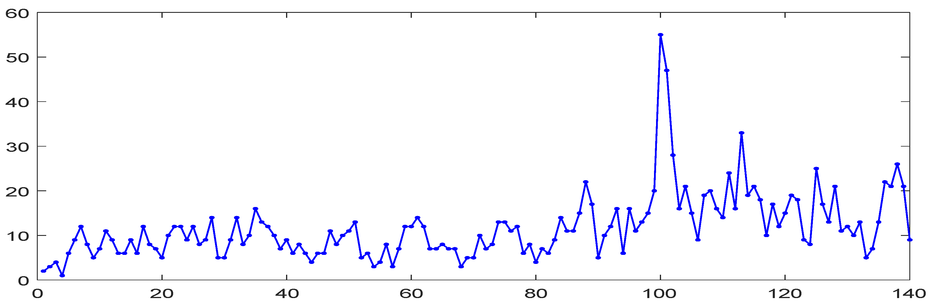
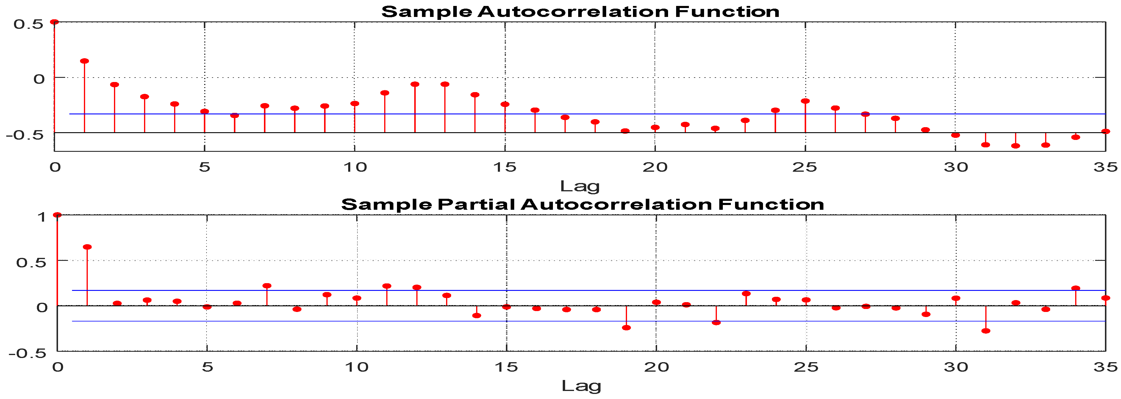
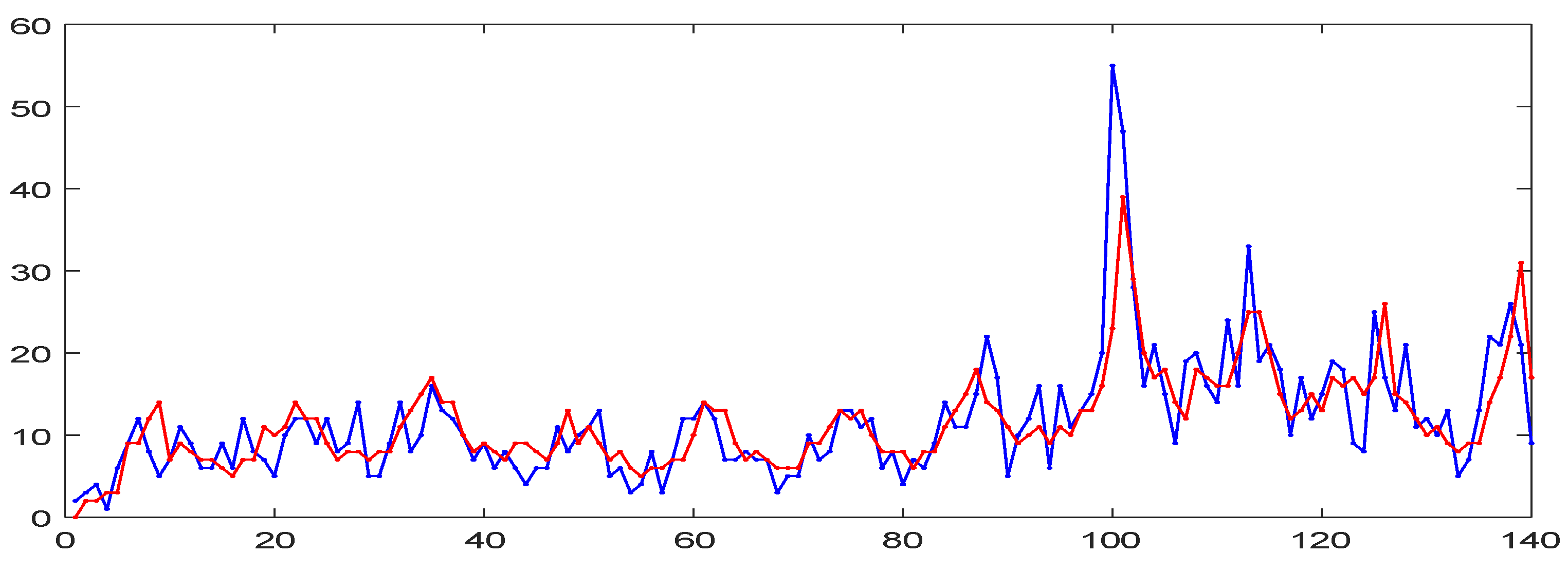
7.2. Empirical Application

The first dataset is number of infections by Campylobacteriosis in Quebec-Canada, from January 1990 to October 2000, consisting in 140 observations, collected every 28 days. The visualization of the Campylobacteriosis time series is shown in Figure 1, while Table 3 summarizes basic descriptive statistics. Figure 2 displays both the empirical autocorrelation function $\left(ACF\right)$ and empirical partial autocorrelation $\left(PACF\right)$ of the dataset.

Figure 1. Campylobacteriosis time series.

Table 3. Descriptive statistics for the Campylobacteriosis time series.

Sample Size	Minimum	Maximum	Median	Mean	Variance	Skewness	Kurtosis
140	1	55	10	$10.6929$	$55.5237$	$2.4981$	$13.2290$

Figure 2. ACF and PACF of the Campylobacteriosis time series.

Table 3 indicates clearly that the data is overdispersed, which indicates that, marginally, a Generalized Poisson distribution is appropriate. The Campylobacteriosis time series, visualized in Figure 1, exhibits a periodical autocorrelation structure, of a period $S=13$, because the date are collected every 28 days, which is confirmed by analyzing its empirical correlogram given by Figure 2. The behaviors of these empirical functions suggest the use of an periodic $GPINGARCH\left(1,1\right)$ model, with period $S=13$. The $CML$ estimates of the periodic parameters, are given in Table 4.

Table 4. The estimated parameters from $PGPINGARC{H}_{13}$(1,1) model.

s	1	2	3	4	5	6	7	8	9	10	11	12	13
${\widehat{\alpha }}_{0,s}$	$0.1817$	$0.0570$	$0.0331$	$0.0477$	$0.7740$	$5.0720$	$0.1220$	$0.1595$	$0.3595$	$4.0128$	$4.9584$	$1.7467$	$0.0521$
${\widehat{\alpha }}_{1,s}$	$0.0607$	$0.7836$	$0.0073$	$0.3408$	$0.0351$	$0.6589$	$0.3673$	$0.1614$	$0.4792$	$0.6301$	$0.0278$	$0.2077$	$0.0039$
${\widehat{\beta }}_s$	$0.9833$	$0.1472$	$0.8422$	$0.9337$	$0.8560$	$0.0200$	$0.6550$	$1.0414$	$0.8273$	$0.0066$	$0.5870$	$0.4381$	$0.8143$
${\widehat{\kappa }}_s$	$0.0029$	$0.1670$	$0.0118$	$0.1477$	$0.0061$	$0.0652$	$0.2080$	$0.0748$	$0.5339$	$0.0885$	$0.0117$	$0.0158$	$0.0032$

In order to assess the adequacy of the fitted model, the standardized Pearson residuals (Weiß et al. 2019 [21]) are used. Therefore, the standardized Pearson residuals of the $PGPINGARC{H}_{13}(1,1)$ model have $0.0154$ mean, and $0.8918$ as variance, which are sufficiently close to 0 and 1, respectively. Additionally, the analysis of the Pearson residuals correlogram, given in Figure 3, do not indicate any significant autocorrelation values. The obtained Ljung-Box statistic value is, $0.6999$, which confirm that there in no evidence of any correlation within the Pearson residuals (because ${\chi }_{0.05,20}^2=31.4140$). Thus, the adequacy of the proposed model is not statistically rejected.

Figure 3. ACF and PACF of Pearson residuals based on the fitted $PGPINGARC{H}_{13}(1,1)$ model.

An estimated trajectory of the process, in red color, opposed to the real data, in blue color, is visualized in Figure 4. It should be noted that the size of our time series is small compared to the number of parameter to estimate which is 52, therefore the selected model can be improved for a larger size.

Figure 4. An adjusted trajectory of the fitted $PGPINGARC{H}_{13}(1,1)$ model.

The fitted $PGPINGARC{H}_{13}(1,1)$ model shows an amelioration comparing to the $INGARCH\left(1,13\right)$ model (Ferland et al. (2006) [1]) and also to the $PINGARC{H}_{13}\left(1,1\right)$ model (Bentarzi and Bentarzi (2017) [15]), in terms of the Sum of Squared Errors $SSE$ and $R^2$ results, computed for each model, listed in Table 5. On the other hand, the fitted $PGPINGARC{H}_{13}(1,1)$ does not show an improvement compared to the Mixture $PINARC{H}_{13}\left(2;1,1\right)$ model (Ouzzani and Bentarzi (2019) [22]), and this is due to the fact that the series seems to be exhibiting a bimodality.

Table 5. Computed SSE and $R^2$ for each model.

	$\mathit{INGARCH}\left(1,13\right)$	${\mathit{PINGARCH}}_{13}\left(1,1\right)$	${\mathit{MPINARCH}}_{13}\left(2;1,1\right)$	${\mathit{PGPINGARCH}}_{13}\left(1,1\right)$
$SSE$	4373	2882	961	2222
$R{}^2$	$83.7187$	$89.2699$	$96.4221$	$91.7271$

8. Conclusions

In this paper we proposed to enlarge the class of $INGARCH$ models so as to include periodicity in their autocovariance structure. The proposed model account for both overdispersion and underdispersion. Periodic mean and variance of the proposed model have been established under some periodically stationary condition. Conditions for the existence higher order moment and their closed forms are shown. The periodic autocovariance structure is considered, while providing the closed-form of the periodic autocorrelation function. The Yule Walker and the Conditional Maximum Likelihood estimators for the periodic parameters are considered. As an illustration, a simulation study was presented, showing the superiority of the $CML$ method. Finally, a real data example, using the $PGPINGARC{H}_S\left(1,1\right)$ model to fit the Campylobacteriosis time series shown an improvement comparing with the exiting models using the same dataset.

References

- Ferland, R.; Latour, A.; Oraichi, D. Integer-valued GARCH process. J. Time Ser. Anal. 2006, 27, 923–942. [Google Scholar] [CrossRef]
- Zhu, F.; Wang, D.; Li, F.; Li, H. Empirical likelihood inference for an integer-valued ARCH(p) model. J. Jilin Univ. Inf. Sci. Ed. 2008, 46, 1042–1048. [Google Scholar]
- Zhu, F.; Li, Q. Moment and Bayesian estimation of parameters in the INGARCH(1, 1) model. J. Jilin Univ. Inf. Sci. Ed. 2009, 47, 899–902. [Google Scholar]
- Fokianos, K.; Rahbek, A.; Tjostheim, D. Poisson autoregression. J. Am. Stat. Assoc. 2009, 104, 1430–1439. [Google Scholar] [CrossRef]
- Fokianos, K.; Fried, R. Interventions in INGARCH processes. J. Time Ser. Anal. 2010, 31, 210–225. [Google Scholar] [CrossRef]
- Doukhan, P.; Leucht, A.; Neumann, M.H. Mixing properties of non-stationary INGARCH(1, 1) processes. arXiv 2020, arXiv:2011.05854. [Google Scholar] [CrossRef]
- Zhu, F. A negative binomial integer-valued GARCH model. J. Time Ser. Anal. 2011, 32, 54–67. [Google Scholar] [CrossRef]
- Zhu, F. Zero-inflated Poisson and negative binomial integer-valued GARCH models. J. Stat. Plan. Inference 2012, 142, 826–839. [Google Scholar] [CrossRef]
- Zhu, F. Modeling overdispersed or underdispersed count data with generalized Poisson integer-valued GARCH models. J. Math. Anal. Appl. 2012, 389, 58–71. [Google Scholar] [CrossRef]
- Zhu, F. Modeling time series of counts with COM-Poisson INGARCH models. Math. Comput. Model. 2012, 56, 191–203. [Google Scholar] [CrossRef]
- McKenzie, E. Autoregressive moving-average processes with negative binomial and geometric marginal distributions. Adv. Appl. Probab. 1986, 18, 679–705. [Google Scholar] [CrossRef]
- McKenzie, E. Some ARMA models for dependent sequences of Poisson counts. Adv. Appl. Probab. 1988, 20, 822–835. [Google Scholar] [CrossRef]
- Al-Osh, M.A.; Alzaid, A.A. First-order integer-valued autoregressive process. J. Time Ser. Anal. 1987, 8, 261–275. [Google Scholar] [CrossRef]
- Weiß, C.H. An Introduction to Discrete-Valued Time Series; Wiley: Chichester, UK, 2018. [Google Scholar]
- Bentarzi, M.; Bentarzi, W. Periodic integer-valued GARCH(1, 1) model. Commun. Stat.-Simul. Comput. 2017, 46, 1167–1188. [Google Scholar] [CrossRef]
- Consul, P.C.; Jain, G.C. A generalization of the Poisson distribution. Technometrics 1973, 15, 791–799. [Google Scholar] [CrossRef]
- Consul, P.C. Generalized Poisson Distributions: Properties and Applications; Marcel Dekker: New York, NY, USA, 1989. [Google Scholar]
- Efron, B. Double exponential families and their use in generalized linear regression. J. Am. Stat. Assoc. 1986, 81, 709–721. [Google Scholar] [CrossRef]
- Gladyshev, E.G. Periodically and almost periodically correlated random processes with continuous time parameter. Theory Probab. Appl. 1963, 8, 173–177. [Google Scholar] [CrossRef]
- White, H. Maximum likelihood estimation of misspecified models. Econometrica 1982, 50, 1–25. [Google Scholar] [CrossRef]
- Weiß, C.; Scherer, L.; Aleksandrov, B.; Feld, M. Checking Model Adequacy for Count Time Series by Using Pearson Residuals. J. Time Ser. Econ. 2019, 12, 20180018. [Google Scholar] [CrossRef]
- Ouzzani, F.; Bentarzi, M. On mixture periodic Integer-Valued ARCH models. Commun. Stat.-Simul. Comput. 2021, 50, 3931–3957. [Google Scholar] [CrossRef]
Disclaimer/Publisher’s Note: The statements, opinions and data contained in all publications are solely those of the individual author(s) and contributor(s) and not of MDPI and/or the editor(s). MDPI and/or the editor(s) disclaim responsibility for any injury to people or property resulting from any ideas, methods, instructions or products referred to in the content. |
© 2023 by the author. Licensee MDPI, Basel, Switzerland. This article is an open access article distributed under the terms and conditions of the Creative Commons Attribution (CC BY) license (https://creativecommons.org/licenses/by/4.0/).