Proceeding Paper

The Asymptotics of Moments for the Remaining Time of Heavy-Tail Distributions †

by
Vladimir Rusev
*,‡ and
Alexander Skorikov
*,‡
Department of Higher Mathematics, National University of Oil and Gas (Gubkin University), 19991 Moscow, Russia
*
Authors to whom correspondence should be addressed.
Presented at the 1st International Online Conference on Mathematics and Applications, 1–15 May 2023; Available online: https://iocma2023.sciforum.net/.
These authors contributed equally to this work.
Comput. Sci. Math. Forum 2023, 7(1), 52; https://doi.org/10.3390/IOCMA2023-14435
Published: 29 April 2023

Abstract

:
Recent mathematical models of reliability computer systems and telecommunication networks are based on distributions with heavy tails. This paper falls into the category of exploring the classical models with heavy tails: Gnedenko–Weibull, Burr, Benktander distributions. The moment’s asymptotics for residual time have been derived especially for there heavy-tailed distributions. A simulation study is presented to give a practice characterization of the distributions with heavy tails.

1. Motivation and Background

Definition 1. 
One defines a cumulative distribution function (DF) F to be (right-) heavy-tailed if and only if
lim x + e λ x F ¯ ( x ) =
for the tail: F ¯ = 1 F and for all λ > 0 .
Thus, one can say that the tail of a distribution (tending to zero) is heavy-tailed if it fails to be bounded by a decreasing exponential function.
Definition 2. 
A cumulative distribution function F is called light-tailed if and only if it fails to be heavy-tailed.
The slow decrease in the tail of a distribution leads to the fact that a random variable can take on very large values with a positive probability. Therefore, such distributions are used to model phenomena that are subject to strong fluctuations. Thus, the sample predominately contains relatively small values, but also has a sufficient number of very large values as illustrated by the plot in Figure 1 for 200 realisations of independent, identically distributed random variables for heavy- (Gnedenko–Weibull DF with less then one shape parameter) and light-tailed (exponential) DF.
Innovated mathematical models of computer systems and telecommunication networks have presented well-characterized heavy-tailed distributions. For example, the superposition of ON/OFF processes with a heavy-tailed distribution was presented in [1]. Such processes converge to a self-similar (fractal) process with self-similarity Hurst exponent H = 3 α / 2 , where 0 < α < 2 is the tail index (or coefficient of heavy-tailedness).
It is well known that there is a correspondence between the generated traffic and actual Ethernet traffic. Empirical self-similar processes of Ethernet traffic remain unchanged at varying time scales unlike Poisson processes, which flatten out as time scales change.
Let X be a non-negative random variable with a cumulative distribution function F. Consider the random variable X t = ( X t X > t ) , which in survival analysis called the residual life time with distribution function F t or distribution of the excess over a threshold t. The function
F ¯ t ( x ) = 1 F t ( x ) = P ( X t > x X > t
is known as the distribution tail. The mathematical expectation of a random variable X t is the mean residual life (MRL) or mean excess function (ME). The ME term is used in risk management, actuarial science and other extreme value problems. This function is defined as
μ ( t ) = E ( X t X > t ) = t + F ¯ ( x ) d x / F ¯ ( t )
and the residual variance (excess variance) is defined by
σ 2 ( t ) = E ( X t 2 ) μ 2 ( t ) = 2 F ¯ ( t ) t + F ¯ ( x ) · μ ( x ) d x μ 2 ( t ) .
The physical application of the MRL to the reliability of the "well–pump" system has been reported in [2].
On the other hand, the accuracy of the simulation obtained depends on the accuracy of the approximation of the distributions with a heavy tail. In model selection it is advisable to study the residual lifetime in terms of its moments for relatively small t. A more precise asymptotic expansion of moments is required. We have obtained new asymptotic expansion terms of the mean excess function (mean residual) and residual variance asymptotic expansion for known distributions.
The paper is organized as follows. In Section 2, we consider the problem of asymptotics of the residual lifetime distribution (mean excess function) for classical models (Tables 1.25, 1.2.6 in [3]). We derive some refinements of asymptotic expansions from (Table 3.4.7 in [3], p. 161). Asymptotic expansions of the residual variance are also obtained.

2. Residual Moments for Heavy Tails

2.1. Gnedenko–Weibull Distribution

The tail two-parameter Gnedenko–Weibull distribution
F ¯ ( t ; α , β ) = e ( α t ) β , t 0
is heavy tailed if 0 < α , 0 < β < 1 .
Let T be a random variable with a two-parameter Gnedenko–Weibull distribution, then α > 0 , β > 0 holds
μ ( t ) = t β α t β 1 + 1 β β α t β + ( 1 β ) ( 1 2 β ) β 2 α t 2 β + O 1 t 3 β , as t ,
σ 2 ( t ) = 1 β 2 α 2 β t 2 ( β 1 ) 1 + 4 ( 1 β ) β ( α t ) β + ( 1 β ) ( 11 17 β ) β 2 ( α t ) 2 β + O 1 t 3 β , as t .
The proof of the asymptotic expressions for the MRL and residual variance is considered in [4].

2.2. Benktander Type I Distribution

The Benktander type I distribution is close to a log normal distribution. These distributions are used to model heavy-tailed losses in actuarial science. Theoretically predicted sizes by Benktander type I distributions are consistent with statistical size distributions in economics and actuarial sciences. The Benktander type I distribution function tail is given by
1 F ( x ) = 1 + 2 β α ln x e β ln x 2 α + 1 ln x , α > 0 , β > 0 , x > 0 .
It then follows that
t 1 F ( x ) d x = t 1 + 2 β α ln x e β ln x 2 α + 1 ln x d x =
= ln t 1 + 2 β α z e β z 2 α + 1 z e z d z = ln t 1 + 2 β α z e β z 2 α z d z =
= ln t 1 + 2 β α z e β z 2 + α β z d z .
Let γ = β α . The mean excess function is directly calculated as:
ln t 1 + 2 γ z e β z 2 + γ z d z = ln t 1 + 2 γ z e β γ γ z 2 + z d z =
= ln t e β γ γ z 2 + z d γ z 2 + z = γ β ln t e β γ γ z 2 + z d β γ γ z 2 + z =
= γ β e β γ γ z 2 + z ln t = γ β e β γ γ ln t 2 + ln t = 1 α e α β α ln t 2 + ln t ;
μ ( t ) = t + 1 F ( x ) d x 1 F ( t ) = 1 α e α β α ln t 2 + ln t 1 + 2 β α ln t e β ln t 2 α + 1 ln t =
= e β ln t 2 t α α + 2 β ln t e β ln t 2 t α 1 = t α + 2 β ln t .
Thus, the Benktander type I distribution has the following exact equality for the mean exceedance:
μ ( t ) = t α + 2 β ln t .
Note that (5) is contained in the Table 3.4.7 in [3], p.161, without proof. The proof is given for completeness.
From the above results and the presentation of the integral
x e z 2 d z = e x 2 1 2 x + 1 4 x 3 + O 1 x 5 , as x ,
it follows
t + ( 1 F ( x ) ) · μ ( x ) d x = 1 α t + e β ln x 2 α + 1 ln x x d x =
= 1 α ln t e β z 2 α + 1 z e 2 z d z = 1 α ln t e β z 2 α z + z d z =
= e α 1 2 4 β α ln t e β z + α 1 2 β 2 d z + α 1 2 β = e α 1 2 4 β α β β ln t + α 1 2 β e u 2 d u =
= e α 1 2 4 β α β e β ln t + α 1 2 β 2 1 2 β ln t + α 1 2 β + 1 4 β ln t + α 1 2 β 3 + .
The residual variance, according to (2) and the above asymptotics, is derives by the equation
σ 2 ( t ) = 2 α α + 2 β ln t · e β ln t 2 + α + 1 ln t · e α 1 2 4 β α β e β ln t + α 1 2 β 2 ×
× 1 2 β ln t + α 1 2 β + 1 4 β ln t + α 1 2 β 3 + O 1 ln t 5 t 2 α + 2 β ln t 2 =
= 2 t 2 α + 2 β ln t · 1 2 β ln t + α 1 + 1 4 β ln t + α 1 2 β 3 + O 1 ln t 5 t 2 α + 2 β ln t 2 =
= t 2 α + 2 β ln t 2 2 β ln t + α 1 1 2 β ln t + α + 4 β 2 2 β ln t + α 1 3 + O 1 ln t 5 =
= t 2 α + 2 β ln t 2 2 β ln t + α + 1 2 β ln t + α 1 2 β ln t + α + O 1 ln t 3 =
= t 2 α + 2 β ln t 2 1 + 2 2 β ln t + α 1 + O 1 ln t 3 as t .
Hence,
σ 2 t = t 2 α + 2 β ln t 2 1 + 2 2 β ln t + α 1 + O 1 ln t 3 ,   as t .
By binomial expansion, one can derive the residual standard deviation
σ ( t ) = t α + 2 β ln t 1 + 1 2 β ln t + α 1 1 4 · 1 2 β ln t + α 1 2 + o 1 ln t 2 ,
as t .

2.3. Benktander Type II Distribution

This distribution is similar to the Gnedenko–Weibull distribution. The formula Benktander type II average residual resource looks like the asymptotics of the average residual resource of the Weibull distribution. However, it is an exact equality, yet for the residual variance there is only an asymptotic expansion. Consider the Benktander type II distribution with distribution tail
1 F ( t ) = e α β t β 1 e α β t β α > 0 , 0 < β < 1 .
It is immediately follows from (1), see Table 3.4.7 in [3]
μ ( t ) = 1 α t 1 β , α > 0 , 0 < β < 1 .
Using the presentation in (9) of μ ( t ) the following formula is derived
t + ( 1 F ( x ) ) · μ ( x ) d x = e α β α t + e α β x β d x .
Substituting z = α β x β into the integral above we obtain
t + e α β x β d x = β 1 β 1 α 1 β α β t β + e z z 1 β 1 d z = β 1 β 1 α 1 β Γ 1 β , α β t β ,
where Γ a , x is an incomplete gamma function:
Γ a , x = 1 Γ a x + e t t a 1 d t .
The presentation in (2) and formula (10) give
σ 2 t = 2 e α β t β 1 e α β t β e α β α β 1 β 1 α 1 β Γ 1 β , α β t β t 2 2 β α 2 .
Thus, for the residual variance an exact equality is obtained using an incomplete gamma function:
σ 2 t = 2 t 1 β e α β t β β 1 β 1 α 1 β + 1 Γ 1 β , α β t β t 2 2 β α 2 .
Formula 8.357 from [5] immediately leads to the expansion of the incomplete gamma function in (10)
Γ 1 β , α β t β =
= α β 1 β 1 t 1 β e α β t β 1 β 1 1 β α t β + β 2 1 1 β 2 1 β α 2 t 2 β + O t 3 β ,
as t .
By inserting asymptotics from the above into (11), it follows that
σ 2 ( t ) =
= 2 t 2 2 β α 1 β 1 α t β + β 1 2 β 1 α 2 t 2 β + O t 3 β t 2 2 β α 2 =
= t 2 2 β α 2 1 2 β 1 α t β + 2 β 1 2 β 1 α 2 t 2 β + O t 3 β , as t .
Finally, the following asymptotic result is found for the residual variance of a Benktander type II distribution
σ 2 t = t 2 2 β α 2 1 2 β 1 α t β + 2 β 1 2 β 1 α 2 t 2 β + O t 3 β , as t ,
and residual standard deviation
σ t = t 1 β α 1 β 1 α 1 t β + β 1 2 β 1 α 2 1 t 2 β + O 1 t 3 β , as t .

2.4. Burr Distribution

The Burr distribution or Burr Type XII distribution (see [6]) is popular as a fit model for a set of insurance data. The following representations are obtained for the Burr distribution moments:
μ ( t ) = t c k 1 1 + c k c k 1 + c · 1 t c + c k 1 c c k 1 + c c k 1 + 2 c · 1 t 2 c + o 1 t 2 c ;
σ 2 ( t ) = c k c k 1 2 · t 2 · 1 c k 2 + 2 c k + 1 c k 1 + c c k 2 + c · 1 t c + o 1 t c , as t .

3. Conclusions

We illustrated the behaviour of the empirical composite samples for some simulated datasets of heavy-tailed distributions in Section 1. The explicit accurate innovated asymptotic expansions were found for the MRL (ME) and residual variance for well-known models from Table 3.4.7 in [3], p. 161. By applying the Balkema de Haan [7] criterion, one may find that these distributions belong (or not) to the attraction exponential distribution.

Author Contributions

Conceptualization, V.R. and A.S.; methodology, V.R.; software, A.S.; validation, V.R., A.S.; formal analysis, V.R.; investigation, V.R.; resources, V.R.; data curation, A.S.; writing—original draft preparation, A.S.; writing—review and editing, V.R.; visualization, A.S.; supervision, V.R.; project administration, V.R.; funding acquisition, A.S. All authors have read and agreed to the published version of the manuscript.

Funding

This research received no external funding.

Institutional Review Board Statement

Not applicable.

Informed Consent Statement

Not applicable.

Data Availability Statement

Not applicable.

Conflicts of Interest

The authors declare no conflict of interest.

Abbreviations

The following abbreviations are used in this manuscript:
DFCumulative distribution function
MRLMean residual life
MEMean excess function
PDFProbability density function

References

  1. Willinger, W.; Taqqu, M.S.; Sherman, R.; Wilson, D.V. Self-Similarity Through High-Variability: Statistical Analysis of Ethernet LAN Traffic at the Source Level. IEEE/ACM Trans. Netw. 1997, 5, 71–86. [Google Scholar]
  2. Dengaev, A.V.; Rusev, V.N.; Skorikov, A.V. The Mean Residual Life (MRL) of the Gnedenko-Weibull Distribution. Estimates of Residual Life Time of Pump Submersible Equipment. Proc. Gubkin Russ. State Univ. Oil Gas 2020, 1/298, 25–37. [Google Scholar] [CrossRef]
  3. Embrechts, P.; Klüppelberg, C.; Mikosch, T. Modelling Extremal Events for Insurance and Finance; Springer: Berlin, Germany, 1997. [Google Scholar]
  4. Rusev, V.; Skorikov, A. Residual Life Time of the Gnedenko Extreme—Value Distributions, Asymptotic Behavior and Applications. In Recent Developments in Stochastic Methods and Applications; Shiryaev, A.N., Samouylov, K.E., Kozyrev, D.V., Eds.; ICSM-5 2020; Springer Proceedings in Mathematics and Statistics; Springer: Berlin/Heidelberg, Germany, 2021; Volume 371, pp. 292–305. [Google Scholar]
  5. Gradshteyn, I.R.; Ryzhik, I.M. Tables of Integrals, Series, and Products; Elsevier Inc.: Oxford, UK, 2007. [Google Scholar]
  6. Rodriges, R. A guide to the Burr type XII distributions. Biometrika 1977, 64, 129–134. [Google Scholar] [CrossRef]
  7. Balkema, A.A.; de Haan, L. Residual life time at great age. Ann. Probab. 1974, 2, 792–804. [Google Scholar] [CrossRef]
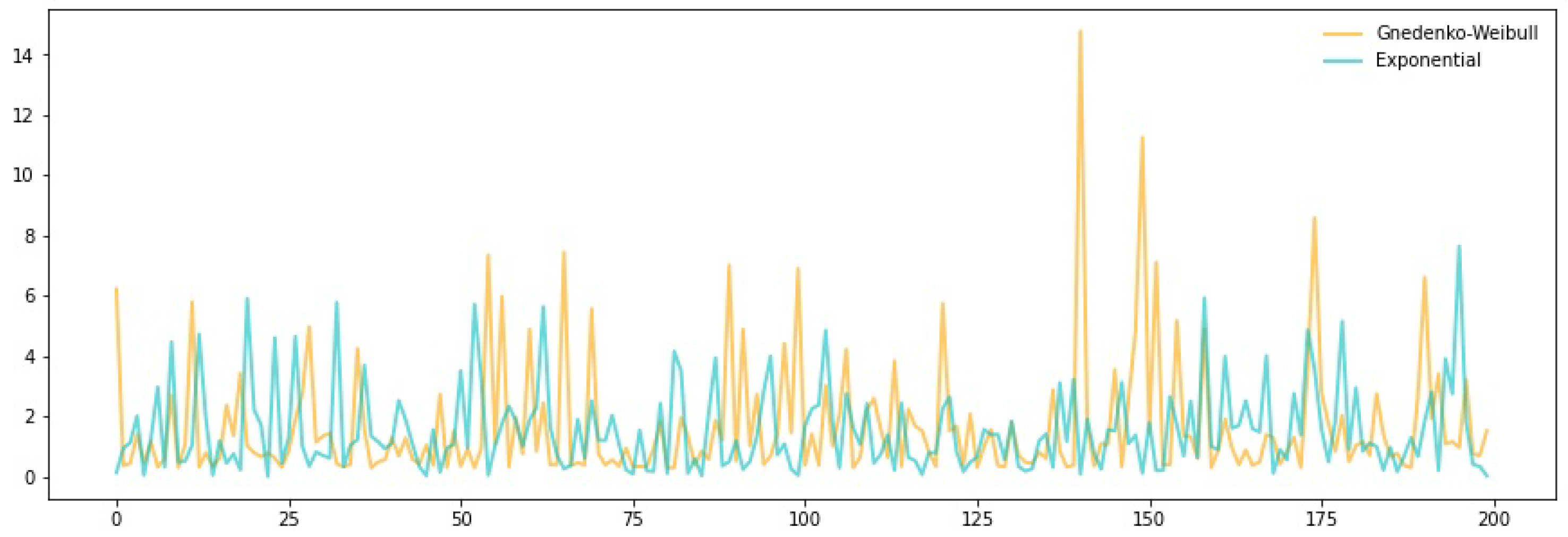
Figure 1. Synthetic plot generated from comparable composite samples of a Gnedenko–Weibull distribution with shape parameter 0.69, scale parameter 1 and exponential distribution with parameter 0.64: Gnedenko–Weibull DF, exponential DF.
Csmf 07 00052 g001
Disclaimer/Publisher’s Note: The statements, opinions and data contained in all publications are solely those of the individual author(s) and contributor(s) and not of MDPI and/or the editor(s). MDPI and/or the editor(s) disclaim responsibility for any injury to people or property resulting from any ideas, methods, instructions or products referred to in the content.