1. Introduction
This study presents a novel method for optimizing functions with angular points or cusps. Several disciplines, such as physics, engineering, finance, and machine learning, encounter this type of issue frequently. The method given reformulates the optimization problem with Euclidean distance as the objective function. The approach is tested with two empirical examples: one employing the absolute value function with a single independent variable and the other with two independent variables. Python’s SciPy module is utilized to implement the stated optimization problems. The outcomes are assessed using two parameters supplied by the optimization solver, specifically the SLQLP algorithm that minimizes the objective function. While the suggested method does not considerably outperform existing techniques, it does offer a viable option for optimizing functions with sharp corners or cusps. Further research could investigate the exact circumstances in which the proposed method performs better, or if there are mathematical, non-heuristic alternatives that could be more effective with this reformulation. Such insights could enhance the efficacy of the proposed strategy and make it a more competitive alternative.
2. Methods
If we consider a function with positive variables and we take into account the segments that go from the
x-axis to the function values, which are internal to the area below the function and above the
x-axis (
Figure 1), then if we identify the longest segment, one of its endpoints will be equal to the maximum value of the function. Based on this idea, we can maximize the Euclidean distance of these segments.
In this study, we empirically evaluate the effectiveness of a reformulation technique for an optimization problem using functions 1 and 2.
Below are the two optimization problems, 3 and 4, in which the two functions, 1 and 2, are present, which become constraints of the problems, and to respect the orthogonality of the segments, we add the equality constraints between the variables that identify the extremum of the segment that is not part of the function of which we are finding the maximum point.
Python Implementation
This section shows how the whole process has been implemented in python using the SciPy library. SciPy is a Python collection of numerical routines that provides the core building blocks for modeling and solving scientific problems. SciPy supports methods for optimization, integration, interpolation, eigenvalue problems, algebraic equations, and differential equations, as well as specific data structures such as sparse matrices and k-dimensional trees [
1].
Optimization problems 3 and 4 are developed in python as in
Figure 2 and
Figure 3, respectively. The code in
Figure 2 defines two functions, func1 and func2, and three constraint functions, constr2, constr4, and constr5. Func1 takes a one-dimensional input x and returns the result of an expression involving x. Func2 takes a three-dimensional input x and returns the result of a mathematical expression involving the components of x. constr2, constr4, and constr5 are constraint functions that take a three-dimensional input x and return the result of an expression that constrains the optimization problem.
The optimization is performed using the minimize function from the scipy.optimize module, with the SLSQP method [
2]. Two sets of optimizations are performed: the first with func1 as the objective function (1), and the second with func2 and the three constraint functions as constraints. The optimization is run multiple times with different values of ftol and eps, and the results are printed to the console.
In
Figure 3, the code performs the same functions as the first in
Figure 2, but more constraints are inserted, and the problem is developed with more variables.
3. Results and Discussion
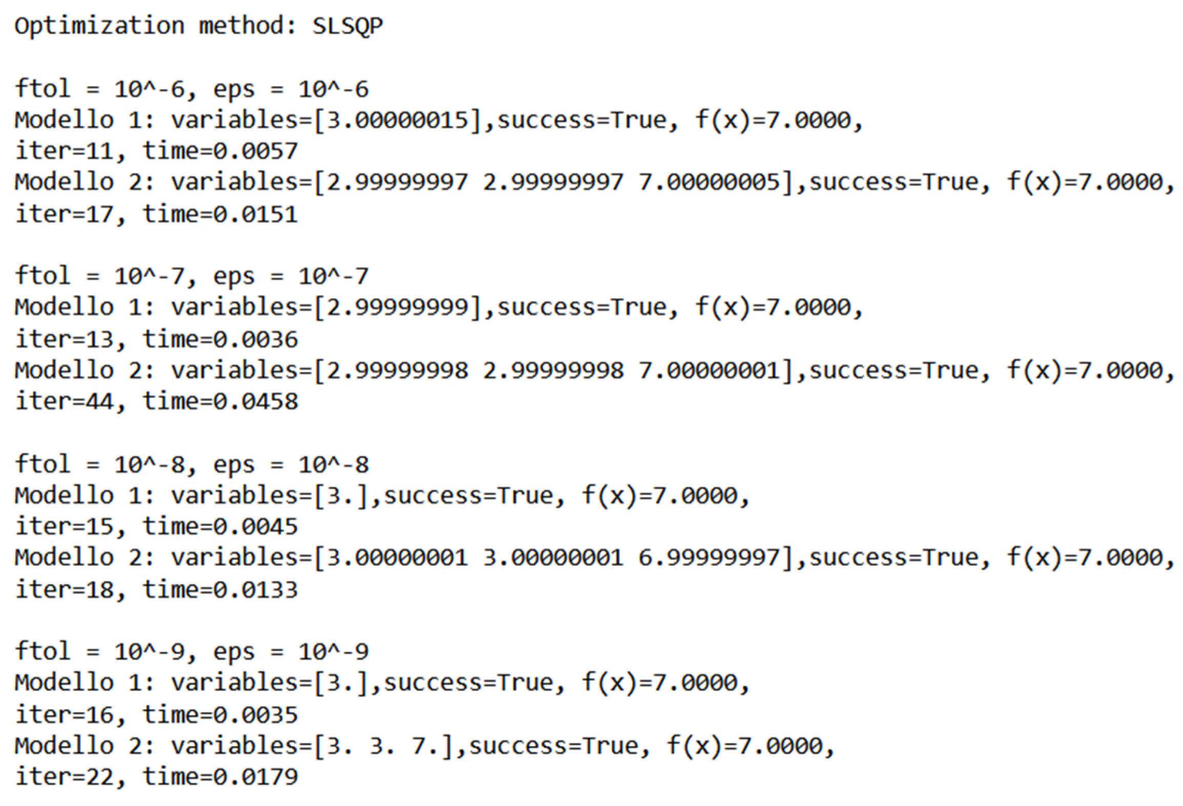
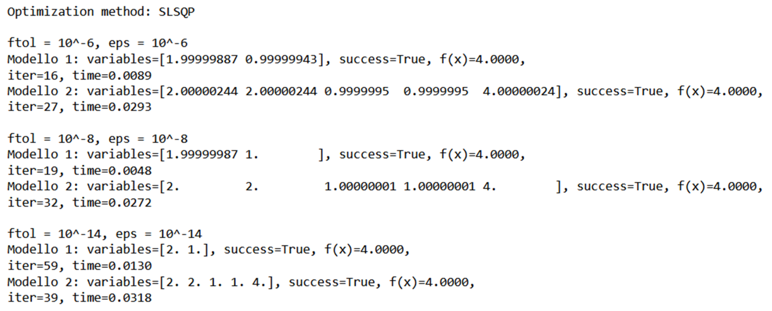
When the value of the ‘success’ parameter is true, this indicates that the optimization is successful and that the proposed method has found a viable solution (
Figure 4 and
Figure 5). This validation method is provided by the SciPy library itself. In
Figure 4 and
Figure 5, the results of the two optimization problems are shown. It is observed that the number of iterations and the elapsed time are lower when the optimization is performed directly without using the proposed method in this work. However, the differences between the two methods are not significant. Moreover, it is noteworthy that for the resolution of the problem, the model formulated with the Euclidean objective function is better for the value of ftol and eps equal to
. This suggests that the choice of objective function and optimization method may depend on the specific problem and the desired level of accuracy. Therefore, it is important to carefully select the appropriate optimization method and tune the parameters to achieve the best results.
Some limitations of the proposed model:
The model assumes that the objective function has a well-defined maximum point, which may not always be the case. Some functions may have multiple local maxima or no maximum at all, making it difficult to identify the global maximum using the proposed approach.
The model requires the generation of a series of segments perpendicular to the abscissa axis, which can be computationally expensive for high-dimensional functions or functions with complex shapes. This could limit the scalability of the approach for larger and more complex optimization problems.
4. Conclusions
In conclusion, further tests and developments are needed to understand if this formulation actually favors a better search for the optimal solution. It is important to explore different combinations of values for ftol and eps and to test the model on a broader range of optimization problems. By doing so, it will be possible to better evaluate the effectiveness and efficiency of this formulation and its potential for future applications.
Author Contributions
Conceptualization, P.F. and M.F.; methodology, P.F.; software, P.F.; validation, M.F.; formal analysis, P.F.; investigation, P.F.; writing—original draft preparation, P.F.; writing—review and editing, P.F.; visualization, P.F.; supervision, M.F.; project administration, M.F. All authors have read and agreed to the published version of the manuscript.
Funding
This research received no external funding.
Institutional Review Board Statement
Not applicable.
Informed Consent Statement
Not applicable.
Data Availability Statement
Not applicable.
Conflicts of Interest
The authors declare no conflict of interest.
References
- Virtanen, P.; Gommers, R.; Oliphant, T.E.; Haberland, M.; Reddy, T.; Cournapeau, D.; Burovski, E.; Peterson, P.; Weckesser, W.; Bright, J.; et al. SciPy 1.0: Fundamental algorithms for scientific computing in Python. Nat. Methods 2020, 17, 261–272. [Google Scholar] [CrossRef] [PubMed]
- Kraft, D. A software package for sequential quadratic programming. Forsch. Dtsch. Forsch. Luft Raumfahrt. 1998, 88, 1–33. [Google Scholar]
| Disclaimer/Publisher’s Note: The statements, opinions and data contained in all publications are solely those of the individual author(s) and contributor(s) and not of MDPI and/or the editor(s). MDPI and/or the editor(s) disclaim responsibility for any injury to people or property resulting from any ideas, methods, instructions or products referred to in the content. |
© 2023 by the authors. Licensee MDPI, Basel, Switzerland. This article is an open access article distributed under the terms and conditions of the Creative Commons Attribution (CC BY) license (https://creativecommons.org/licenses/by/4.0/).


