Patterns in a Time-Fractional Predator–Prey System with Finite Interaction Range ^†

Abstract

Diffusive predator–prey systems are well known to exhibit spatial patterns obtained by using the Turing instability mechanism. reaction–diffusion systems were already studied by replacing the time derivative with a fractional order derivative, finding the conditions under which spatial patterns could be formed in such systems. The recent interest in fractional operators is due to the fact that many biological, chemical, physical, engineering, and financial systems can be well described using these tools. This contribution presents a diffusive predator–prey model with a finite interaction scale between species and introduces temporal fractional derivatives associated with species behaviors. We show that the spatial scale of the species interaction affects the range of unstable modes in which patterns can appear. Additionally, the temporal fractional derivatives further modify the emergence of spatial patterns.

1. Introduction

In population dynamics, Lotka–Volterra equations describe a system of two coexisting species whose densities oscillate in time [1]. These systems can exhibit diffusion-driven instabilities, which are explained by the Turing mechanism for diffusion-reaction systems [2,3], through extensions or modifications of the original model [4,5,6]. Predator–prey interaction is a multi-factor dependent process. For instance, some studies consider hunting cooperation, prey defense mechanisms, limited localized resources, and cross-diffusion terms for studying the influence of movements on both species [7].

It has been proposed that the relative distance between a predator and prey can influence the probability of an encounter between them. The latter is modeled through a nonlinear reactive term that considers the mean of the possible interactions within a fixed radius centered on one of the two species [8,9]. These finite-range interaction models show that the emergence of patterns is not only driven by diffusion but also there are regions where the instability is driven by the interaction range [8]. Recently, this model has been extended by introducing a constant drift and constraining the system to a large and narrow environment [10]. In such an analysis, the geometry of the boundaries induces an effect that couples with the drift. Thus, the corresponding dispersion relation has three parameters: the ratio of diffusivities, a dimensionless drift, and the ratio of interaction lengths, which enlarge the parameter space and, therefore, the possibilities of obtaining different kinds of spatio-temporal patterns.

On the other hand, many processes, not only in ecology but in many other areas, have been adequately described through models that include equations with fractional time derivatives, which are well-known to model memory and non-local effects [11]. Including such effects, beyond just modifying the nonlinear interaction terms, brings the model closer to a more realistic situation [12]. For reaction–diffusion models with anomalous diffusion, it has been seen that the parameter that drives the instability is modified by the anomalous diffusion exponent [13]. The inclusion of temporal fractional derivatives in predator–prey systems has been shown to help control the stability of patterns for species coexistence [14]; memory effects can also shift the bifurcation threshold in such systems [15]. It has also been shown that in systems where patterns do not naturally emerge, fractional derivatives can induce diffusion-driven instability and thus pattern formation, hence the importance of using this kind of model [16,17].

In general, the changes induced by fractional time derivatives in reaction–diffusion systems have been extensively studied in the literature [18,19,20,21,22]. In almost all cases, it was found that the nonlinearity of the functions describing the kinetics had an essential role in the generation of spatial and temporal patterns.

In this work, we are interested in finding a relationship between the fractional derivative and the Turing instability, that is, if the temporal fractional derivative induces Turing instability and produces spatial patterns. We present the stability analysis of the model that considers the mean number of interspecies interactions in a given region defined by the interaction distance. This distance is one of the parameters guiding the system towards the instability leading to pattern formation. We consider whether replacing the time derivative by a fractional operator accounts for memory effects in a predator–prey diffusive model with a finite interaction scale between species.

The manuscript is structured as follows. Section 2 analyzes the predator–prey model with a finite interaction length. We find the steady state and the corresponding dispersion relation that depends on three parameters. The instability curve for the control parameter is found when the ratio of the characteristic lengths of each species is larger than two, which is the set value in previous studies. Section 3 presents the system’s stability analysis when a fractional operator replaces the time derivative to account for memory effects, and its consequences are discussed. Section 4 summarizes the obtained results.

2. Predator–Prey Model with Finite Interaction Length

Let us consider a model characterized by a system of two equations: one for the prey $N(x,t)$ and one for the predator $P(x,t)$. They describe diffusion in the physical space, and the strength of the interaction (nonlinear term) is a function of individuals’ proximity. These reaction–diffusion models with the spatial interaction scale have been widely applied to model the competition of species’ coevolution in an ecology community. We introduce two different length scales to consider different effective interaction ranges, the region where prey and predators interact may have different relevance to predator growth and prey death. These scales have an important role in pattern formation. The model is as follows:

$$\begin{array}{ccc}\hfill \frac{\partial N(x,t)}{\partial t}& =& D_N\frac{{\partial }^{2}N(x,t)}{\partial x^2}+rN(x,t)-\alpha N(x,t){\int }_{x-L_1}^{x+L_1}P(s,t)ds,\hfill \end{array}$$

(1)

$$\begin{array}{ccc}\hfill \frac{\partial P(x,t)}{\partial t}& =& D_P\frac{{\partial }^{2}P(x,t)}{\partial x^2}-mP(x,t)+\beta P(x,t){\int }_{x-L_2}^{x+L_2}N(s,t)ds.\hfill \end{array}$$

(2)

Predators consume the prey with an intrinsic rate $\alpha$ and reproduce with the rate $\beta$; r is the growth rate of prey, and predators are assumed to die spontaneously with rate m. $D_N$ and $D_P$ are the constant diffusion coefficients of prey and predators, respectively. The conditions under which the spatio-temporal patterns occur are first studied considering the stationary case with no diffusion. This gives us the stationary state $(\overline{N},\overline{P})=(m/\left(2\beta L_2\right),r/\left(2\alpha L_1\right))$. By considering now small harmonic perturbations for both species, we pbtain the following dispersion relation of the system with diffusion

$$\widehat{\lambda }\left(K\right)=-K^2+\frac{\sqrt{rm}{L}_1^2}{DK}\sqrt{-{sin}^{2}KcosK}.$$

(3)

where $D_N=D_P=D$, $L_2=2L_1$, $K=k{L}_1$, and $\widehat{\lambda }=\lambda \frac{L_1^2}{D}$. The system was further studied in [10], and it was found that a general dispersion relation is the following:

$$\widehat{\lambda }=-\frac{(1+d)}{2}\left(K^2\right)\pm \frac{1}{2}{\left[{(1-d)}^2{K}^4-4{\mu }^2\frac{sin\left(K\right)sin(K\ell )}{K^2\ell }\right]}^{1/2},$$

(4)

from now on $\widehat{\lambda }=\lambda \frac{L_1^2}{D_N}$, and the parameters $d=D_P/D_N$, $\mu =\sqrt{rm}{L}_1^2/D_N$, and $\ell =L_2/L_1$ were introduced. Certainly if $d=1$ and $\ell =2$, this reduces to the above expression.

The system (1) and (2) linearized around the stationary point, with no diffusion, leads to a characteristic equation $\widehat{\lambda }=\pm i\mu$, two conjugate imaginary eigenvalues, which is the limiting case for the instability condition since it has no real part. As the eigenvalues are purely imaginary and conjugate to each other, this fixed point must be a center for closed orbits in the local vicinity, i.e., an attractive or repulsive spiral in the phase space.

Turing Instability Parameter Space

For several values of $\mu$, it has been seen that the critical value $d_c$ is reached for values close to 1; therefore, when increasing, there will be no pattern formation. For ℓ, something similar happens; it has been seen that to guarantee pattern formation, $\ell \ne 1$ must be fulfilled, and usually it is just considered $\ell =2$, as in Equation (3). However, it is not the only possible value.

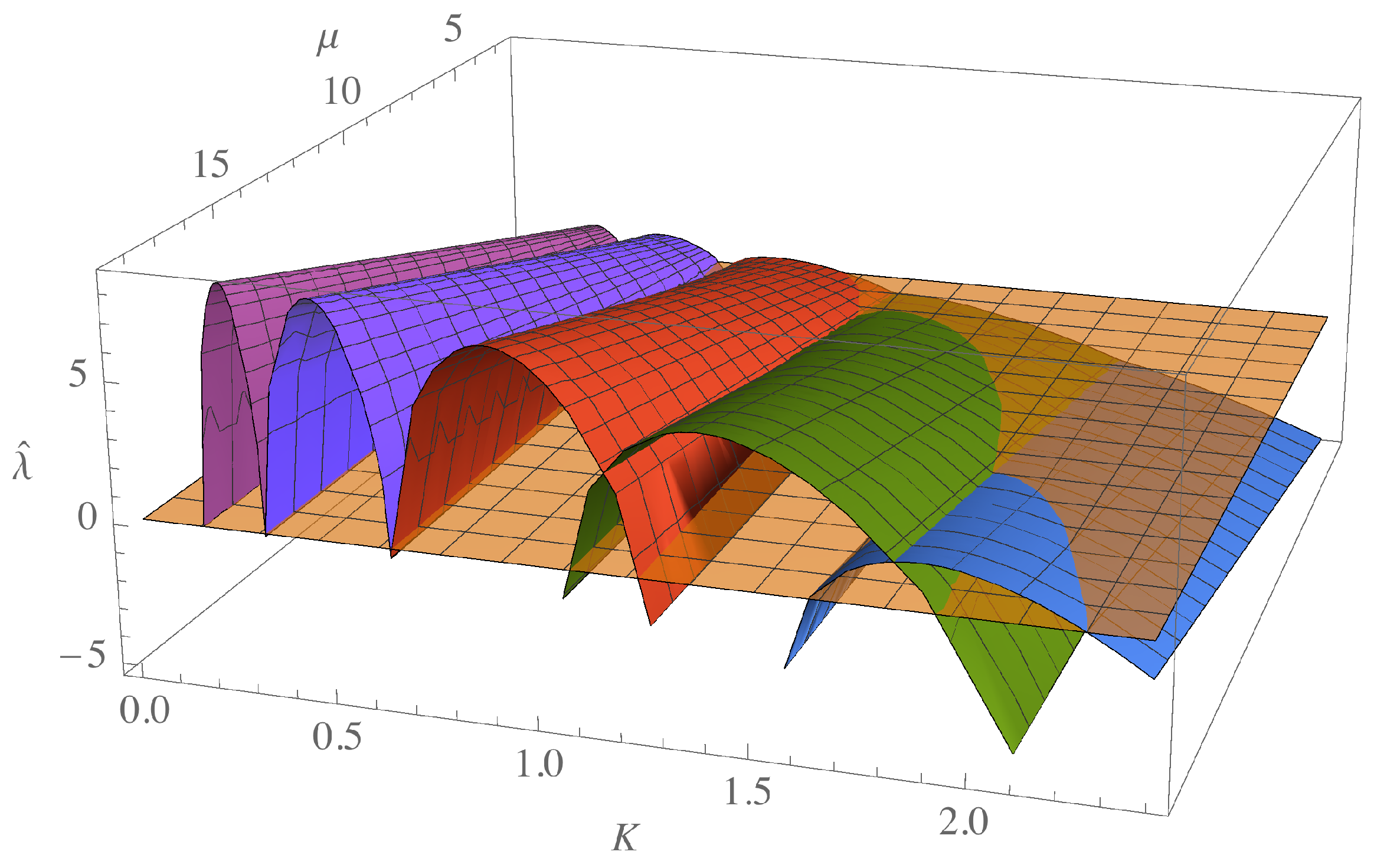
In Figure 1, we plot the dispersion relation (4) with $d=1$, as a function of K, varying the parameter $\mu$ and for different values of ℓ indicated with different colors. This figure shows that as ℓ increases, different ranges of unstable modes appear for each fixed $\mu$ value. The choice of values $\ell >2$ increases the space of possibilities that meet the instability condition and pattern formation.

To satisfy the instability condition $\mathrm{Re}\left(\lambda \right(K\left)\right)<0$ for pattern formation, it is usually necessary to verify the so-called Turing conditions [2], a number of inequalities that come from the analysis of the dispersion relation. This is equivalent to considering the instability threshold when ${\widehat{\lambda }}_c=0$ in the characteristic equation, imposing a relation among the system parameters and the critical value $K_c$, which determines such a threshold. For Equation (4), we find that the parameters to study the instability of the system will be $(\mu ,\ell )$. Remember that $\mu$ measures the competition of time scales given by the species’ growth, death, and diffusion rates, while ℓ is the ratio between the characteristic lengths. Choosing ${\mu }^2$ as the control parameter [23], it is possible to obtain the following relation, having fixed $d=1$,

$${\mu }^2(K,\ell )=-\frac{\ell K^6}{sin\left(K\right)sin(K\ell )}.$$

(5)

This expression has a minimum in $K_c$ obtained by deriving and equaling zero; this reduces to solving the next equation, and as we can see it will depend on the choice of ℓ,

$$K_c(cot\left(K_c\right)+\ell cot(K_c\ell ))=0.$$

(6)

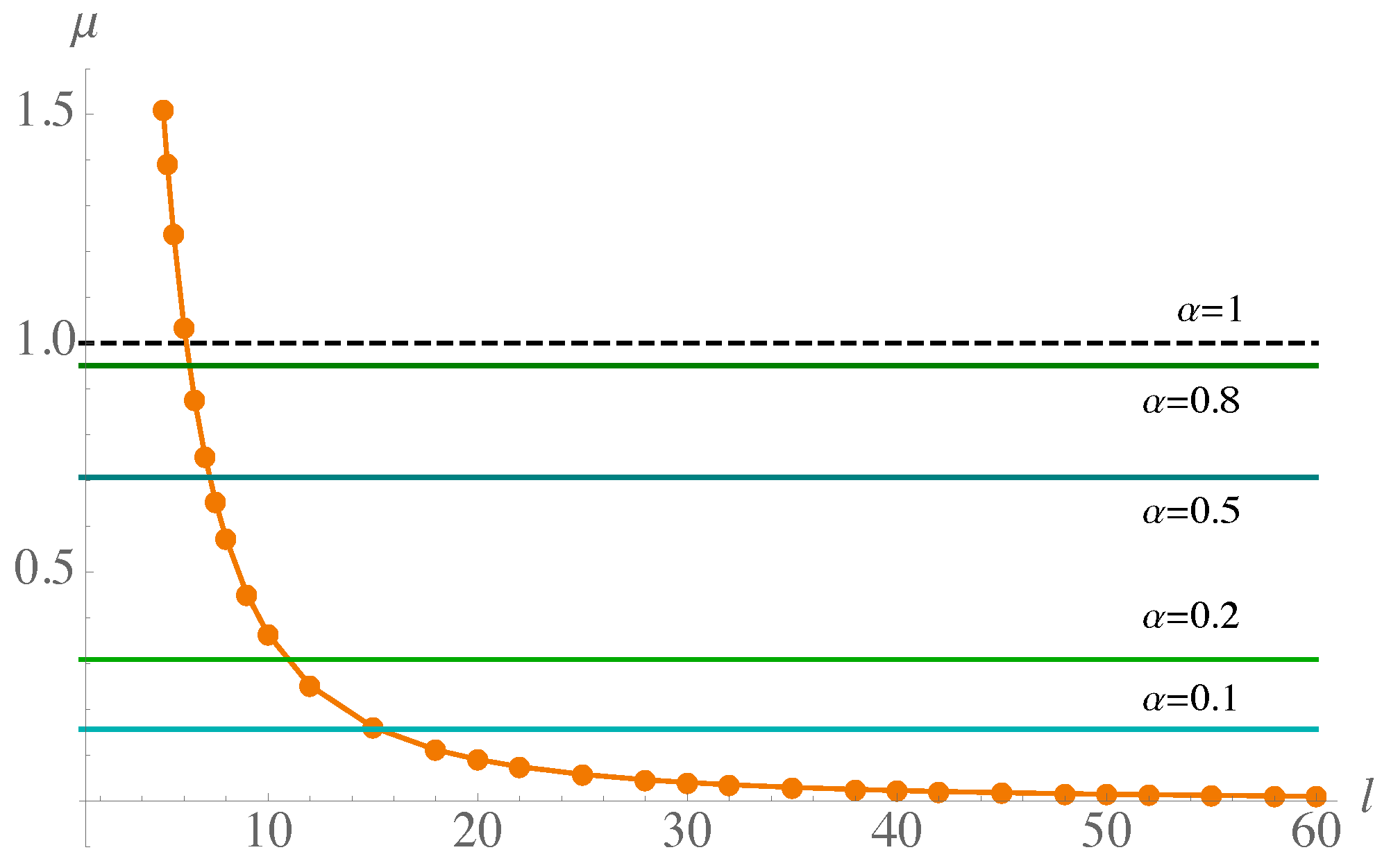
We can construct the stability curve ${\mu }_c(\ell )$ in parameter space, which satisfies the above equations, such that patterns will emerge for values greater than the critical value of the control parameter $\mu >{\mu }_c$. See the orange dots and curve in Figure 2.

The ratio of the interaction lengths of the two species ℓ, as mentioned in [8], is an important parameter since it drives the instability together with d. As we can see in Figure 2, as ℓ increases, the parameter $\mu$ decreases but does not vanish.

3. Fractional-Order System Stability Analysis

Let us now consider a reaction–diffusion system of fractional order in the temporal derivative

$$\begin{array}{ccc}\hfill \frac{{\partial }^{\alpha }N(x,t)}{\partial t^{\alpha }}& =& D_N\frac{{\partial }^{2}N(x,t)}{\partial x^2}+f(N,P),\hfill \end{array}$$

(7)

$$\begin{array}{ccc}\hfill \frac{{\partial }^{\alpha }P(x,t)}{\partial t^{\alpha }}& =& D_P\frac{{\partial }^{2}P(x,t)}{\partial x^2}+g(N,P),\hfill \end{array}$$

(8)

where f, g are usually nonlinear functions, and in this case we will consider the same dynamics as in (1) and (2). The fractional time derivative is defined in Caputo’s sense as

$$\frac{{\partial }^{\alpha }F\left(t\right)}{\partial t^{\alpha }}:=\frac{1}{\Gamma (1-\alpha )}{\int }_0^t\frac{\partial F\left(t^{\prime }\right)}{\partial t^{\prime }}\frac{d{t}^{\prime }}{{(t-t^{\prime })}^{\alpha }},$$

(9)

with $0<\alpha <1$, which is defined by its Laplace transform as follows:

$$\widehat{\mathcal{L}}\left\{\frac{{\partial }^{\alpha }F\left(t\right)}{\partial t^{\alpha }}\right\}=s^{\alpha }\tilde{F}\left(s\right)-s^{\alpha -1}F(0+),$$

where $\tilde{F}\left(s\right)=\widehat{\mathcal{L}}\left\{F\left(t\right)\right\}$, and $0<\alpha <1$.

To study the stability of the system, we first consider the diffusionless case. Let $\mathcal{P}=(\overline{N},\overline{P})$ be an equilibrium point of the system; its the stability of can be determined by linearizing the system (7) and (8) around it, which leads to the following linear system:

$$\left(\begin{array}{c}\frac{{\partial }^{\alpha }\overline{N}(x,t)}{\partial t^{\alpha }}\\ \\ \frac{{\partial }^{\alpha }\overline{P}(x,t)}{\partial t^{\alpha }}\end{array}\right)=\underset{\mathbf{A}}{\underbrace{{\left(\begin{array}{cc}{f}_u& f_v\\ g_u& g_v\end{array}\right)}_{\mathcal{P}}}}\left(\begin{array}{c}\overline{N}\\ \overline{P}\end{array}\right).$$

(10)

By transforming the system to Laplace space, it is possible to rearrange it as follows:

$$\underset{\Delta \left(s\right)}{\underbrace{\left(\lambda \left(s\right)\mathbf{I}-\mathbf{A}\right)}}(\mathcal{L}\left(\overline{N}\right),\mathcal{L}\left(\overline{P}\right))=(\mathcal{L}\left\{\overline{N}\left(0\right)\right\},\mathcal{L}\left\{\overline{P}\left(0\right)\right\})s^{\alpha -1},$$

(11)

where $\lambda \left(s\right)=s^{\alpha }$. The equilibrium point $\mathcal{P}$ of the system is stable if all the roots of the characteristic equation $\Delta \left(s\right)=0$ have negative real part, i.e., $\mathrm{Re}\left(\lambda \right)<0$, additionally to satisfying the usual conditions [2,23]. In the complex plane, the negativity condition means that the argument of s must be greater than $\frac{\pi }{2}$; this implies that the argument of $\lambda$ must be

$$|arg\left(\lambda \right)|>\alpha \frac{\pi }{2},$$

(12)

this is called the Mantignon form for the stability criterion for the fractional case [24,25].

For the system (1) and (2), it was shown that, in the absence of diffusion, $\mu =sin\left(arg\left(\widehat{\lambda }\right)\right)$; condition (12) implies that $\mu >{\mu }_{\alpha }=sin(\alpha \pi /2)$, which defines a constraint surface in the extended parameter space $(\mu ,\ell ,\alpha )$, such that, besides satisfying the condition seen above $\mu >{\mu }_c$, this condition must also be fulfilled to guarantee the stability of the steady state associated with the order $\alpha$.

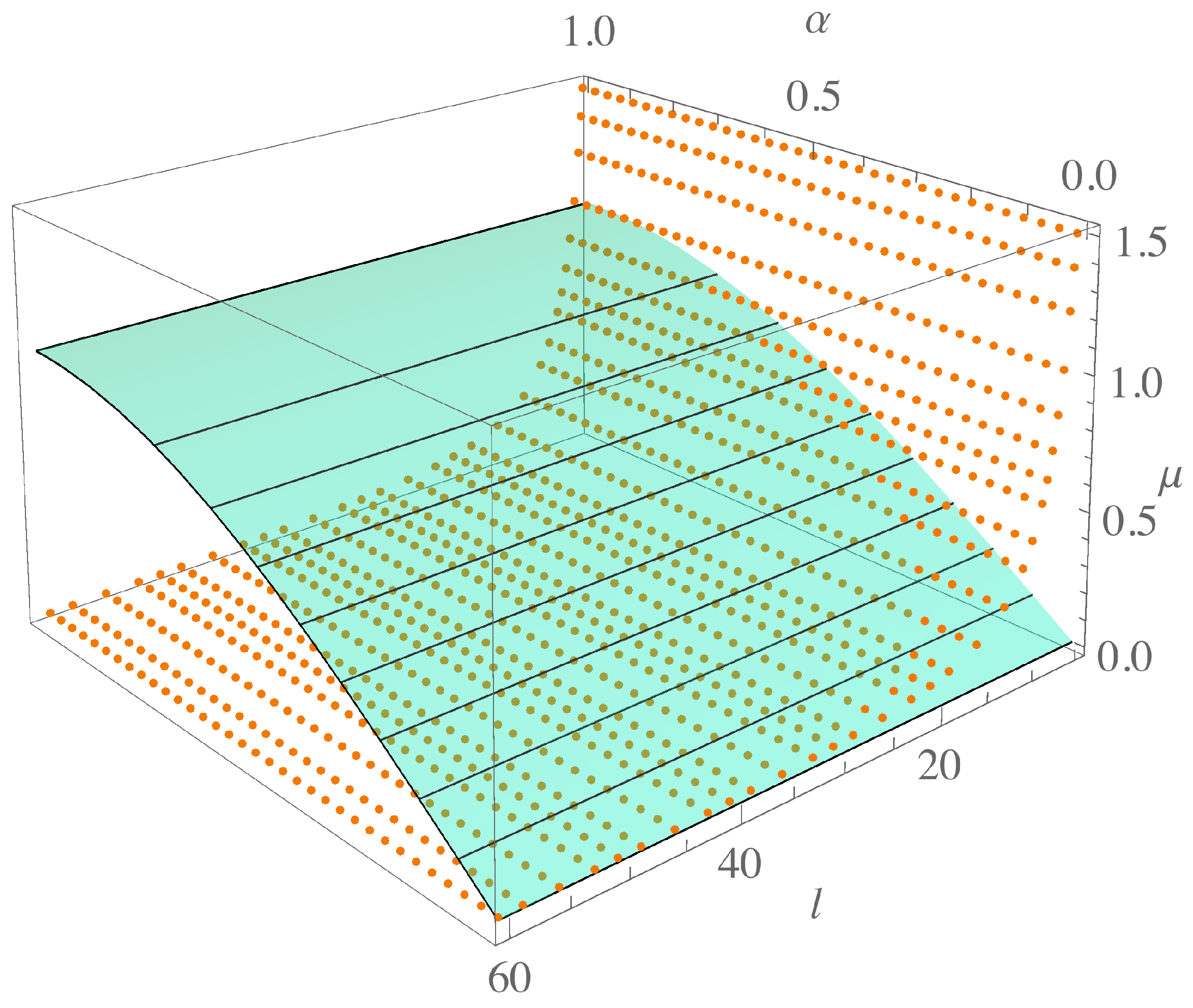
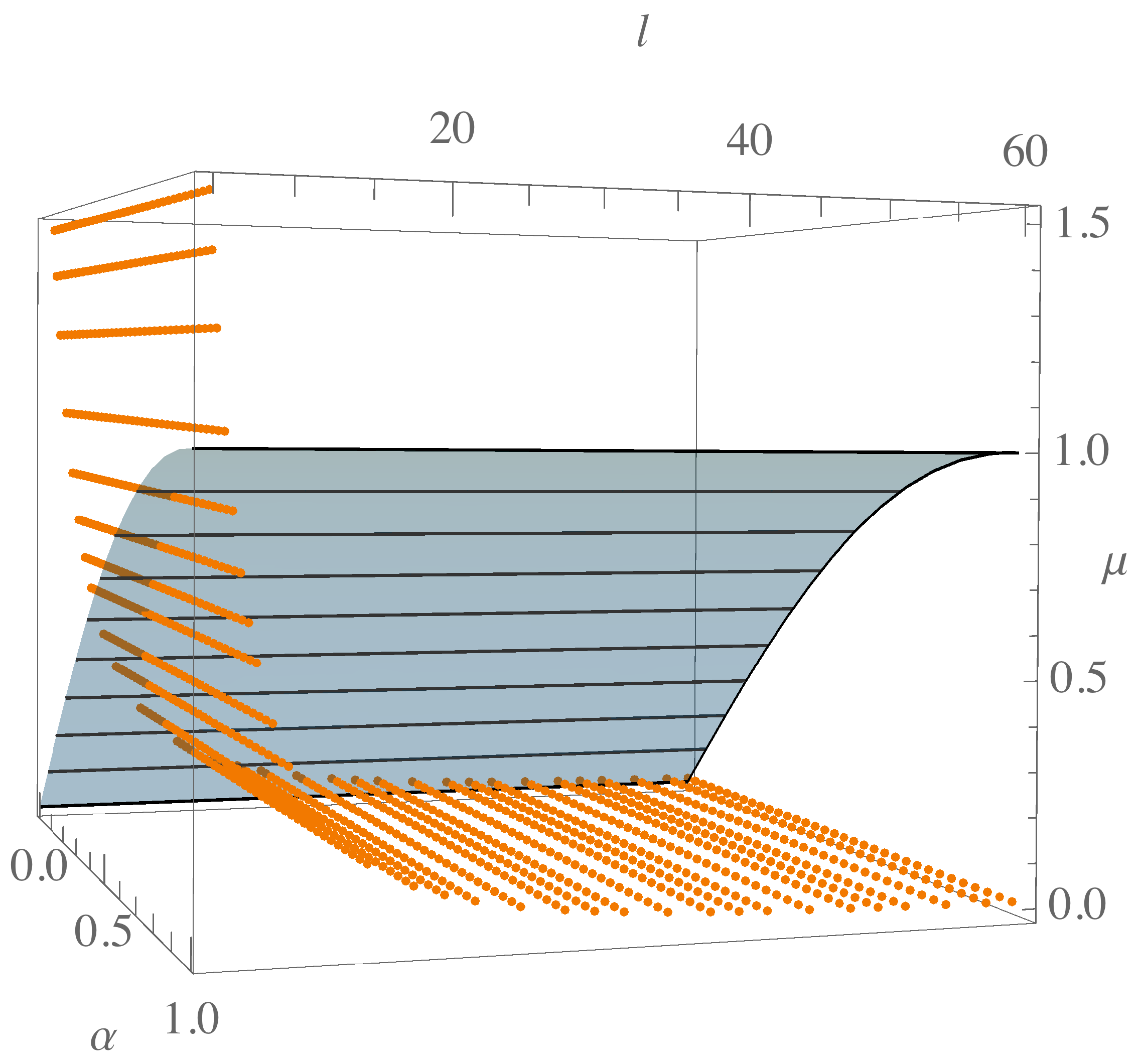
In Figure 2, Figure 3 and Figure 4, the effect of this constraint can be seen. In Figure 2, ${\mu }_c(\ell )$ is plotted, so to guarantee pattern formation $\mu$ must take values above this curve. Considering different values of $alpha$, we see that for larger $ell$, the values of $m{u}_c(\ell )$ must be beyond those determined by $m{u}_c(\ell )$., i.e., there will be a region associated with the order $\alpha$, given by ${\mu }_{\alpha }>{\mu }_c$, for which the parameter values that previously met the instability conditions are now discarded, and pattern formation is no longer possible.

Notably, for the extreme case $\alpha =1$, condition (12) merely reduces to asking for $\mu >1$ values. Although this condition does not influence the non-fractional case, it does set an upper bound on the values of $\mu$ dropped by the fractional order. This case is illustrated as a dotted line in Figure 2. The interesting point is that its intersection with the curve ${\mu }_c$, which occurs at approximately ${\ell }_{*}\approx 6$, indicates the values of ℓ above from which the fractional order will have an effect, depending on the value of $\alpha$. In Figure 3 and Figure 4, the intersection of the two surfaces ${\mu }_c$ and ${\mu }_{\alpha }$ in the extended parameter space is shown for each value of $\alpha$. The region below the surface is just the region discarded by the fractional order of the system, while the intersection curve gives the minimum ℓ for each $\alpha$.

4. Conclusions

Over the last few years, it has been seen that many physical, chemical, and biological systems, where memory effects cannot be neglected, are well described through reaction–diffusion equations with fractional time derivatives. This work presents the stability analysis of a reaction–diffusion system when a fractional operator replaces the time derivative.

Early analyses found that this distance is indeed one of the parameters guiding the system towards the instability that leads to pattern formation [8,9]. Later studies showed that the parameter space for studying this instability could be extended to include drift effects, as well as the large values of the characteristic length ratio and the parameter $\mu$ that is a combination of the birth and death rates of the species and the characteristic time at which they diffuse [10].

Introducing the fractional time operator to include memory effects restricts the time eigenvalue as a function of the fractional order of the derivative, in addition to the well-known conditions. Thus, on the one hand, it is necessary to extend the parameter space to include the fractional order. However, on the other hand, since several conditions must be fulfilled simultaneously, the intersections of the restriction surfaces must be found to find the corresponding critical values. In the specific case of the predator–prey system, this is reflected in the fact that for large values of the characteristic length ratio—values approximately greater than six—the value of $\mu$ must be taken above the critical value given by the Turing conditions. How large this value should be depends on the fractional order. That is, there is a region of $\mu$ values that in the usual case can form patterns but at the order $\alpha$ is forbidden. When the interaction lengths of the species are very different, memory effects cause the $\mu$ values that are suitable for pattern formation to be reduced.

The class of oscillations and their behavior will be analyzed in future work. The present study reinforces the importance of the influence of the anomalous order in the formation of unsteady state structures in a system where diffusivity is not the only parameter guiding instabilities.