Dynamic Analysis for the Physically Correct Model of a Fractional-Order Buck-Boost Converter ^†

Abstract

This work proposes a fractional-order mathematical model of a Buck-Boost converter performing in continuous conduction mode. To do so, we employ the average duty-cycle representation in state space, driven by the nonadimensionalize approach to avoid unit inconsistencies in the model. We also consider a Direct Current (DC) analysis through the fractional Riemann–Liouville (R-L) approach. Moreover, the fractional order Buck-Boost converter model is implemented in the Matlab/Simulink setting, which is also powered by the Fractional-order Modeling and Control (FOMCON) toolbox. When modifying the fractional model order, we identify significant variations in the dynamic converter response from this simulated scenario. Finally, we detail how to achieve a fast dynamic response without oscillations and an adequate overshoot, appropriately varying the fractional-order coefficient. The numerical results have allowed us to determine that with the decrease of the fractional order, the model presents minor oscillations, obtaining an output voltage response six times faster with a significant overshoot reduction of 67%, on average.

1. Introduction

Modern power electronics techniques aim to provide an efficient way to transform electrical energy [1]. One is a Direct Current (DC–DC) voltage converter [2], which transforms an input voltage into an output voltage of a different magnitude, preserving its exact nature. The main goal is to supply a regulated voltage with a minimum ripple. DC–DC converters are switched sources that transform the input voltage to the desired output value with elements that intrinsically make the system non-linear. These converters are widely used, especially as power supplies in computer hardware and medical equipment [3]. The adequate control of the output voltage of these converters has been an essential subject of study during the last few years. Therefore, the switching operation is mainly responsible for their non-linear behavior and increasing design complexity [4,5].

The literature is prolific in studying integer-order models of DC–DC converters. Nevertheless, the capacitor and inductor could behave depending on fractional derivatives [1,6]. Therefore, fractional order models provide a more accurate description and deeper insight into physical processes [7,8]. In recent years, there has been significant study and development of fractional order systems [9,10]. Unfortunately, the inconsistency of units at the time of modeling is often overlooked when trying to model these electronic elements. There are three most used definitions of fractional calculus: Caputo Derivative (CD), Riemann–Liouville (R-L) fractional integral, and Grünwald–Letnikov (G-L) derivative [11]. Because of differences between the fractional calculus definitions, the model results under different fractional orders may present variations related to the used fractional derivative and the occasional requirement of initial conditions.

This work analyzes the fractional order model of a Buck-Boost converter, its system is nondimensionalized, and its properties are in Continuous Conduction Mode (CCM). In doing so, we first nondimensionalized the fractional-order model of such a converter represented in the state space. Next, we consider the converter’s duty cycle to achieve an average model in the state–space of fractional order. Afterward, we analyze the non-linear nature of the Buck-Boost converter fractional representation to determine the values for which the converter’s performance increases.

The main contributions of the proposed Fractional-order Buck-Boost model were a decrease in the output voltage oscillations or harmonics, fast settling time, and a nondimensionalized version of the inductor current and capacitor voltage responses at a stable state.

2. Mathematical Modeling

This section describes the mathematical procedure we followed for analyzing and modeling the fractional-order Buck-Boost converter. First, we detail the most relevant aspects of the traditional converter model using classical calculus. Then, we apply the non-dimensionalization procedure to achieve a physically correct model.

2.1. DC–DC Buck-Boost Converter

The DC–DC Buck-Boost converter is derived from the combination of elementary converters such as Buck and Boost. The resulting configuration can provide an output voltage of inverse polarity, either greater or smaller than the input voltage. In this study, we replace the integer-order capacitor and inductor with fractional-order ones to transform the traditional converter model into the fractional domain. 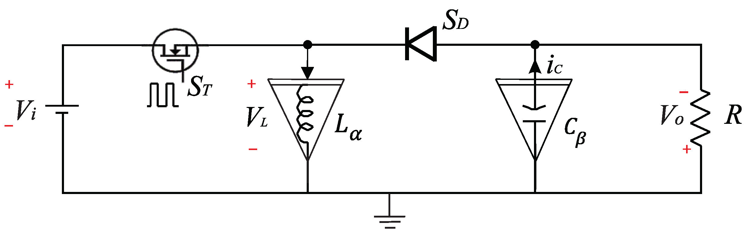Figure 1 shows the circuit based on non-integer calculus representing the fractional-order Buck-Boost converter.

Figure 1. Fractional-order Buck-Boost converter.

In this circuit, R [$\Omega$] corresponds to the load, $Vi$ [V] stands for the input voltage, $S_T$ represents an ideal switching power MOSFET, and $S_D$ an ideal diode. In a broad sense, the converter works as follows: when it operates in CCM, it appears in two switching states defined below.

• State 1: $S_T=\mathrm{ON}$ and $S_D=\mathrm{OFF}$, for $nT<t\le (n+D_c)T$.
• State 2: $S_T=\mathrm{OFF}$ and $S_D=\mathrm{ON}$, for $(n+D_c)T<t\le (n+1)T$.

In both states, n is an integer, T is the switching period, and $D_c$ is the duty cycle of the Pulse Width Modulation (PWM) commuting $S_T$, which is defined as the ratio between the turn-on time of $S_T$ and T. Hence, States 1 and 2 switch periodically in a stable state. In practice, obtaining a fractional model of the capacitor and inductor is possible based on the pioneering analysis performed by Zhang et al. [12] and Jiang and Zhang [13]. Consequently, the inductor’s voltage $v_L$ and the capacitor’s current $i_c$ can be represented using a fractional model, such as,

$$\begin{array}{ccc}\hfill & v_L\left(t\right)=L\frac{d^{\alpha }{i}_L}{d{t}^{\alpha }},\hfill & \hfill i_C\left(t\right)=C\frac{d^{\beta }{v}_C}{d{t}^{\beta }},\end{array}$$

(1)

where $\alpha$ and $\beta$ denote the fractional order of the derivatives for the inductor’s current $i_L$ and capacitor’s voltage $v_c$, respectively.

This model contains two features worth noticing. The former is when $\alpha =\beta =1$, so the inductor and the capacitor components behave as ideal electronic components of integer order derivatives. The latter is when $\{\alpha ,\beta \}\in (0,1)$ presents a fractional order.

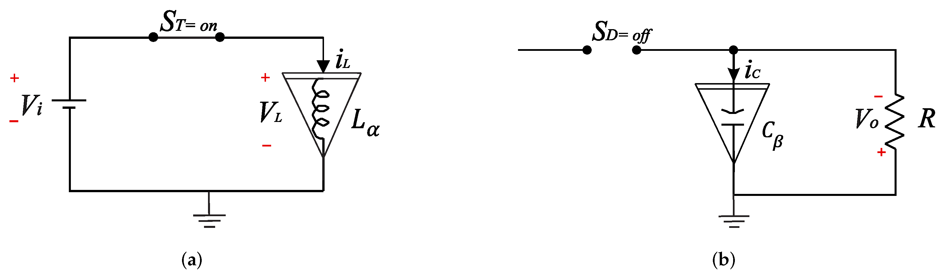
Considering the particular case when $S_T=\mathrm{ON}$ and $S_D=\mathrm{OFF}$, the fractional-order Buck-Boost converter turns into State 1.

Applying Kirchhoff’s voltage law over the equivalent circuits of Figure 2, it is easy to obtain,

$$\begin{array}{ccc}\hfill & L\frac{d^{\alpha }{i}_L}{d{t}^{\alpha }}=V_i,\hfill & \hfill C\frac{d^{\beta }{v}_C}{d{t}^{\beta }}=-\frac{v_C}{R}.\end{array}$$

(2)

Figure 2. Equivalent circuits of the Buck-Boost converter in State 1 with $S_T=\mathrm{on}$ and $S_D=\mathrm{off}$. (a) Equivalent circuit of the Buck-Boost converter in State 1 and $S_T=\mathrm{ON}$. (b) Equivalent circuit of the Buck-Boost converter in State 1 and $S_D=\mathrm{OFF}$.

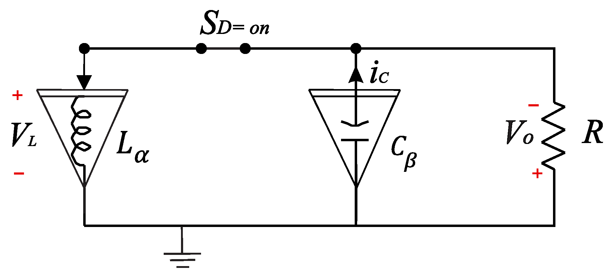
Meanwhile, when the $S_T=\mathrm{OFF}$ and $S_D=\mathrm{ON}$, the fractional-order Buck-Boost converter is in State 2, as Figure 3 depicts.

Figure 3. Equivalent circuit of the Buck-Boost converter in State 2 with $S_T=\mathrm{OFF}$ and $S_D=\mathrm{ON}$.

Performing a Kirchhoff’s voltage law analysis on the equivalent circuit in Figure 3, the fractional-order differential equations supporting the State 2 analysis are,

$$\begin{array}{cc}\hfill & L\frac{d^{\alpha }{i}_L}{d{t}^{\alpha }}=-v_C,\hfill \\ \hfill & C\frac{d^{\beta }{v}_C}{d{t}^{\beta }}=i_L-\frac{v_C}{R}.\hfill \end{array}$$

(3)

Merging (2) and (3) and implementing the state-space averaging model of the fractional-order Buck-Boost converter operating in CCM leads to the next coupled model:

$$\begin{array}{cc}\hfill & L\frac{d^{\alpha }{⟨i_L⟩}_T}{d{t}^{\alpha }}=S_D{⟨V_i⟩}_T-(1-S_D){⟨v_C⟩}_T,\hfill \\ \hfill & C\frac{d^{\beta }{⟨v_C⟩}_T}{d{t}^{\beta }}=-\frac{{⟨v_C⟩}_T}{R}+(1-S_D){⟨i_L⟩}_T.\hfill \end{array}$$

(4)

From these expressions, it is essential to recall that ${⟨x⟩}_T$, for any $x\left(t\right)$, is the average value of this variable x during a switching period, and it can be numerically computed as follows,

$${⟨x⟩}_T=\frac{1}{T}{\int }_t^{t+T}x\left(t\right)dt.$$

(5)

2.2. Fractional-Order DC–DC Buck-Boost Converter

It is well-known that circuit variables in the converter, such as inductor’s current $i_L$ and capacitor’s voltage $v_c$, present high-order harmonics due to the commutation sequence related to the operating principle of the Buck-Boost converter. These harmonics are eliminated by averaging the circuit variables, considering a switching period. Furthermore, when linearizing the model and obtaining the system transfer function, the averaged model of the converter is given by,

$$\begin{array}{cc}\hfill & L\frac{d^{\alpha }{i}_L}{d{t}^{\alpha }}=D_c{V}_i-(1-D_c)v_c,\hfill \\ \hfill & C\frac{d^{\beta }{v}_c}{d{t}^{\beta }}=-\frac{v_c}{R}+(1-D_c)i_L.\hfill \end{array}$$

(6)

Since a fractional-order derivative is used, such a transformation procedure generates inconsistency in the units of the model depending on the chosen operator [14]. Consequently, it is paramount to apply a nonadimensionalize procedure to render fractional-order differential equations with dimensions physically correct. Next, the characteristic parameters used to nonadimensionalize are

$$\begin{array}{ccc}\hfill {\displaystyle \widehat{\tau }=\frac{t}{L/R}}& ⟶& {\displaystyle dt=\frac{L}{R}d\widehat{\tau },}\hfill \\ \hfill {\displaystyle \widehat{\varphi }=\frac{i_L}{V_i/R}}& ⟶& {\displaystyle d{i}_L=\frac{v_i}{R}d\widehat{\varphi },}\hfill \\ \hfill {\displaystyle \widehat{\psi }=\frac{v_c}{V_i}}& ⟶& {\displaystyle d{v}_c=V_{i}d\widehat{\psi }.}\hfill \end{array}$$

(7)

Therefore, the nondimensional model is obtained by substituting (7) into (6), as follows

$$\begin{array}{cc}\hfill & \frac{d^{\alpha }\widehat{\varphi }}{d{\widehat{\tau }}^{\alpha }}=-(1-D_c)\widehat{\psi }+D_c,\hfill \\ \hfill & \frac{d^{\beta }\widehat{\psi }}{d{\widehat{\tau }}^{\beta }}=k_{\tau }\left[-\widehat{\psi }+(1-D_c)\widehat{\varphi }\right],\hfill \end{array}$$

(8)

where $k_{\tau }=\frac{L/R}{RC}$ is a constant produced by nondimensionalizing (6).

As in the integer case, the fractional state–space model is defined by two equations [15]:

• A state equation, where each state $x_i\left(t\right)$ is differentiated to a fractional-order ${\alpha }_i$, is given in the case of a generalized state–space model. All states $x_i\left(t\right)$ are differentiated to the same fractional order $\alpha$ for the commensurate case.
• An output equation depends on the internal states and the inputs, as in the integer case.

Before obtaining the fractional state–space model, we first applied the concept of fractional derivative to the classic state–space representation. In consequence, such a fractional model in the state–space domain corresponds to

$$\begin{array}{cc}\hfill D^{\left(\alpha \right)}\left(x\right)& =A_{s}x+B_{s}u,\hfill \\ \hfill y& =C_{s}x+D_{s}u,\hfill \end{array}$$

(9)

where $D^{\left(\alpha \right)}\left(x\right)={\left[D^{{\alpha }_1}{x}_1,D^{{\alpha }_2}{x}_2,\dots ,D^{{\alpha }_n}\right]}^{⊺}$, since $A_s$, $B_s$, $C_s$, and $D_s$ are the state–space representation model matrices. Roughly speaking, we can obtain any model in the Laplace domain by using its transform and considering zero initial conditions,

$$G\left(s\right)=C_s\left[{\left(s^{\alpha }{I}_n-A_s\right)}^{-1}\right]B_s+D_s,$$

(10)

where $D_s$ is generally null. The fractional state–space model, derived from (8), is now defined as

$$\left[\begin{array}{c}{\displaystyle \frac{d^{\alpha }\widehat{\varphi }}{d{\widehat{\tau }}^{\alpha }}}\\ {\displaystyle \frac{d^{\beta }\psi }{d{\widehat{\tau }}^{\beta }}}\end{array}\right]=\underset{A_s}{\underbrace{\left[\begin{array}{cc}{\displaystyle 0}& -(1-D_c)\\ k_{\tau }(1-D_c)& -k_{\tau }\end{array}\right]}}\left[\begin{array}{c}\widehat{\varphi }\\ \widehat{\psi }\end{array}\right]+\underset{B_s}{\underbrace{\left[\begin{array}{c}{D}_c\\ 0\end{array}\right]}}u\left(t\right),y=\underset{Cs}{\underbrace{\left[\begin{array}{cc}1& 0\\ 0& 1\end{array}\right]}}\left[\begin{array}{c}\widehat{\varphi }\\ \widehat{\psi }\end{array}\right].$$

(11)

For the sake of simplicity, we assume that $\alpha =\beta$. Thus, the proposed transfer function is obtained from (11) as follows,

$$M=s^{\alpha }I-A_s=\left[\begin{array}{cc}{s}^{\alpha }& (1-D_c)\\ -k_{\tau }(1-D_c)& s^{\alpha }+k_{\tau }\end{array}\right],$$

(12)

where the characteristic equation is given by

$$\left|M\right|=s^{2\alpha }+k_{\tau }{s}^{\alpha }+{(1-D_c)}^2{k}_{\tau },$$

(13)

$$G\left(s\right)=\frac{1}{s^{2\alpha }+k_{\tau }{s}^{\alpha }+k\tau {(1-D_c)}^2}\left[\begin{array}{cc}1& 0\\ 0& 1\end{array}\right]\left[\begin{array}{cc}{s}^{\alpha }+k_{\tau }& -(1-D_c)\\ k_{\tau }(1-D_c)& s^{\alpha }\end{array}\right]\left[\begin{array}{c}{D}_c\\ 0\end{array}\right].$$

(14)

$$G\left(S\right)=\left[\begin{array}{c}{\displaystyle \frac{D_c(s^{\alpha }+k_{\tau })}{s^{2\alpha }+k_{\tau }{s}^{\alpha }+{(1-D_c)}^2{k}_{\tau }}}\\ {\displaystyle \frac{k_{\tau }{D}_c(1-D_c)}{s^{2\alpha }+k_{\tau }{s}^{\alpha }+{(1-D_c)}^2{k}_{\tau }}}\end{array}\right]U\left(S\right),$$

(15)

where $U\left(S\right)=\mathcal{L}\left\{u\right(t\left)\right\}$ is the Laplace transform of $u\left(t\right)$. Once the system of equations is nondimensionalized, we can express the output $\widehat{\varphi }$ and $\widehat{\psi }$ as follows,

$$\begin{array}{ccc}\hfill \widehat{\varphi }\left(s\right)& =& \frac{D_c\left(s^{\alpha }+k_{\tau }\right)U\left(s\right)}{s^{2\alpha }+k_{\tau }{s}^{\alpha }+{(1-D_c)}^2{k}_{\tau }},\hfill \end{array}$$

(16)

$$\begin{array}{ccc}\hfill \widehat{\psi }\left(s\right)& =& \frac{k_{\tau }{D}_c(1-D_c)U\left(s\right)}{s^{2\alpha }+k_{\tau }{s}^{\alpha }+{(1-D_c)}^2{k}_{\tau }}.\hfill \end{array}$$

(17)

3. Stable-State Analysis

The linearized model (6) is solved using the definition of the Riemann–Liouville derivative, defined as

$${}_a^{\mathrm{RL}}{D}_b^{\alpha }f\left(t\right)=\frac{1}{\Gamma (1-\alpha )}\frac{d}{dt}{\int }_a^b\frac{f\left(t\right)}{{(t-\tau )}^{\alpha }}d\tau ,$$

(18)

where $\Gamma (·)$ is the Gamma function and [a, b] is the interval of the stable-state signal.

Thereby, the fractional derivatives of the variables $i_L$ and $v_c$ are obtained from (18), respectively, as shown,

$$\begin{array}{cc}\hfill & \frac{d^{\alpha }{i}_L}{d{t}^{\alpha }}=\frac{1}{\Gamma (1-\alpha )}\frac{d}{dt}{\int }_{nT}^{(n+1)T}\frac{i_L}{{(t-\tau )}^{\alpha }}d\tau =\frac{i_L{t}_s^{-\alpha }}{\Gamma (1-\alpha )},\hfill \\ \hfill & \frac{d^{\beta }{v}_c}{d{t}^{\beta }}=\frac{1}{\Gamma (1-\beta )}\frac{d}{dt}{\int }_{nT}^{(n+1)T}\frac{v_c}{{(t-\tau )}^{\beta }}d\tau =\frac{v_c{t}_s^{-\beta }}{\Gamma (1-\beta )},\hfill \end{array}$$

(19)

where n is the current operating cycle of the PWM, $t_s$ is the time needed so that the Buck-Boost converter achieves the stable state. Once the converter reaches this state, the inductor current ($i_L$) and capacitor voltage ($v_c$) are considered constant and $t_s\approx T$.

Substituting (19) in (6), the inductor current and capacitor voltage at stable state are defined as,

$$\begin{array}{ccc}\hfill i_L& =& \frac{V_i{D}_c\left[RC{t}_s^{-\beta }+\Gamma (1-\beta )\right]}{\Gamma (1-\beta )R{(1-D_c)}^2+\frac{L{t}_s^{-\alpha }\Gamma (1-\beta )}{\Gamma (1-\alpha )}+\frac{RCL{t}_s^{-(\beta +\alpha )}}{\Gamma (1-\alpha )}},\hfill \end{array}$$

(20)

$$\begin{array}{ccc}\hfill v_c& =& \frac{V_i{D}_c(1-D_c)R\Gamma (1-\beta )\Gamma (1-\alpha )}{R\Gamma (1-\beta )\Gamma (1-\alpha ){(1-D_c)}^2+\Gamma (1-\beta )L{t}_s^{-\alpha }+RLC{t}_s^{-(\alpha +\beta )}}.\hfill \end{array}$$

(21)

The Buck-Boost converter voltage ratio $G_v$ at stable state is obtained by (20) since the capacitor voltage is directly the output voltage,

$$G_v=\frac{v_c}{V_i}=\frac{D_c(1-D_c)R\Gamma (1-\beta )\Gamma (1-\alpha )}{R\Gamma (1-\beta )\Gamma (1-\alpha ){(1-D_c)}^2+\Gamma (1-\beta )L{t}_s^{-\alpha }+RLC{t}_s^{-(\alpha +\beta )}}.$$

(22)

Table 1 presents the circuit parameters used in the numerical simulations and the fractional-order converter model analysis in the stable state.

Table 1. Parameters used for the simulations to obtain the Buck-Boost converter fractional model response in the stable state.

Parameter	Values
Stable–state time	$t_s=T=4$ ms
Input voltage	$V_i=25$ V
Inductor	$L=3$ mH
Capacitor	$C=150$ $\mathsf{\mu }$F
Load	$R=30\Omega$
Duty cycle	$D_c=0.6$

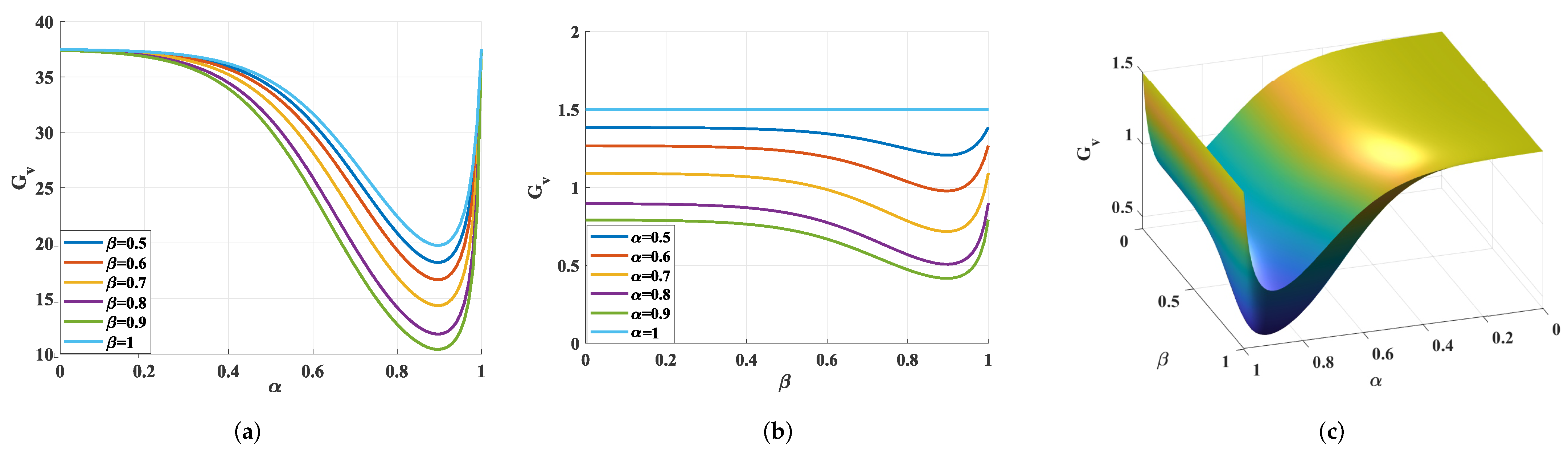
Figure 4 displays the response of the Buck-Boost converter fractional model in the stable state. Plus, in Figure 4b, we fixed $\alpha$, varying the value of $\beta$. Notice that the $G_v$ response falls slowly but then recovers rapidly. Figure 4a is the opposite case. When varying $\beta$, the $G_v$ response tends to mimic the behavior shown in Figure 4b. Additionally, Figure 4c shows the dynamic variation of the $G_v$ with the change of the fractional order, presenting a minimum gain when $\alpha =\beta =0.956$.

Figure 4. Visualization of $\alpha$ and $\beta$ influence the response of $G_V$ in stable-state. (a) Relationship between $G_v$ and $\alpha$. (b) Relationship between $G_v$ and $\beta$. (c) Three-dimensional representation of $\alpha$ and $\beta$ variations.

4. Numerical Simulation

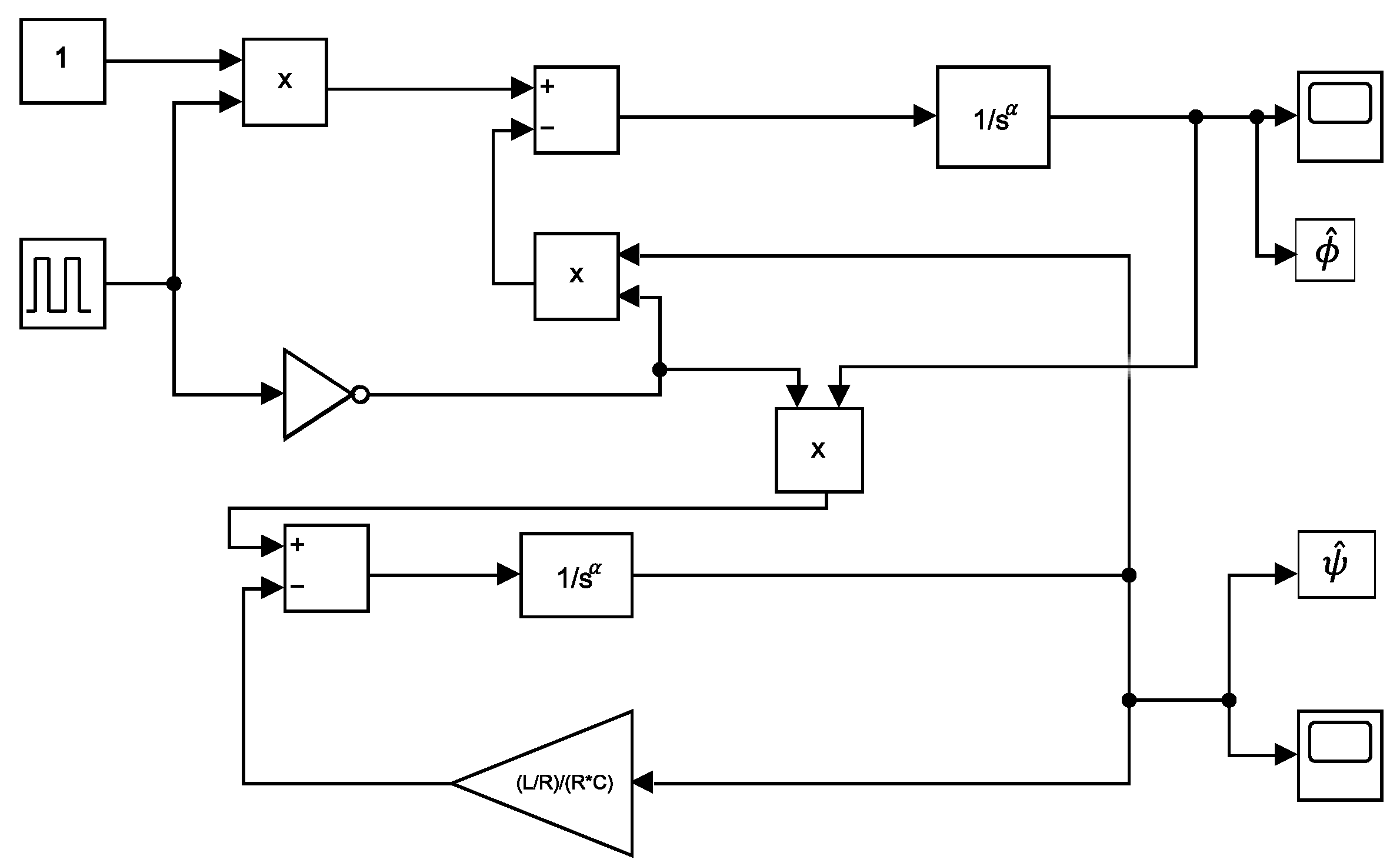
The mathematical model of the fractional-order Buck-Boost converter driven by CCM is implemented in the Matlab/Simulink environment through the FOMCON toolbox [16]. According to the state–space model given by (11), we construct the block diagram of the system, as shown in Figure 5. It is noteworthy that $1/s^{\alpha }$ is the fractional integral unit.

Figure 5. Numerical simulation of the fractional mathematical model by Matlab/Simulink.

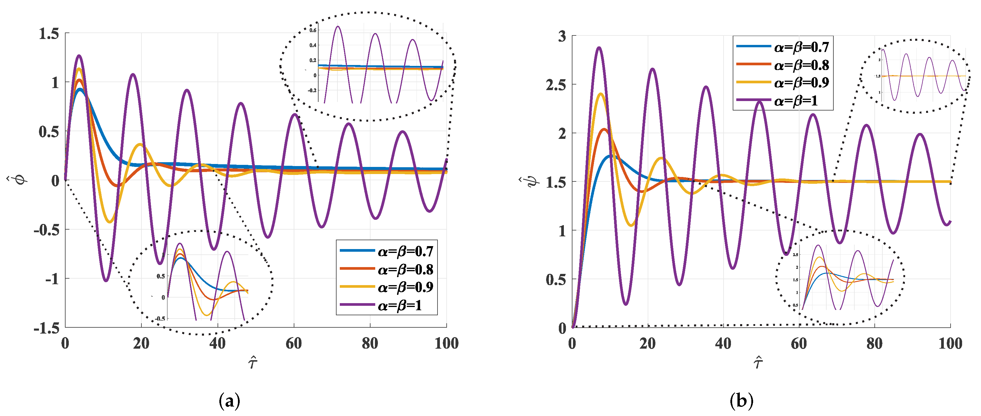
The parameters for this numerical simulation were previously given in Table 1. Furthermore, Figure 6 shows the dynamic response of $\widehat{\varphi }$ and $\widehat{\psi }$, cf. (7), which are associated with the nondimensionalized inductor current ($i_L$) and capacitor voltage ($v_C$), respectively.

Figure 6. Nondimensionalized voltage and current of the fractional-order Buck-Boost converter. (a) Nondimensionalized inductor’s current. (b) Nondimensionalized capacitor’s voltage.

Figure 6a displays the behavior of the nondimensionalized inductor current with different $\alpha$ values. It is worth commenting that when $\alpha =0.7$, $i_L$ achieves the desired behavior, exhibiting a lower overshoot without negative values.

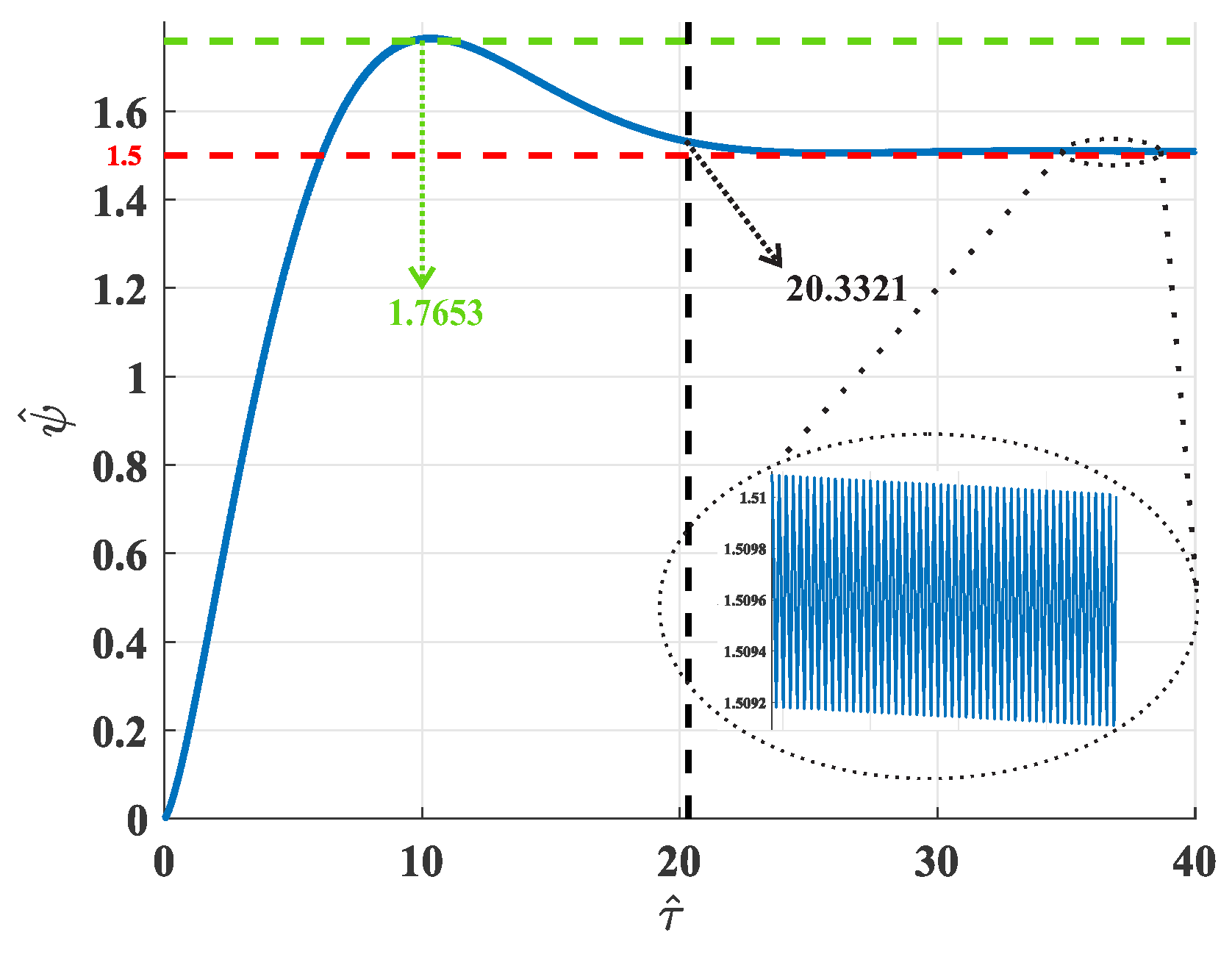
Figure 6b shows the nondimensionalized capacitor voltage under different scenarios. We noticed that when the fractional order tends to unity, we obtain the traditional responses of the converter, containing a myriad of oscillations. Further, the converter must evolve for a long time to reach the desired reference. However, when $\alpha$ begins to decrease, this reference is tracked in a shorter time. A similar behavior occurs with the nondimensional inductor’s current for the nondimensional voltage when $\alpha =0.7$, as Figure 7 shows. The obtained output is the desired one in this type of converter: a smooth and controlled voltage rise, a lower overshoot concerning the other solutions, and a fast settling time.

Figure 7. Nondimensionalized capacitor voltage with $\alpha =0.7$.

The red dotted line represents the voltage reference value set in $1.5$. The green dotted line represents the maximum peak reached by the converter, which has a value of $1.7653$ that translates into an overshoot of $17.6854$%. The black dotted line corresponds to the reached settling time by this device, which is equal to ${\widehat{t}}_{ss}=20.3321$, using the criterion of 5%. Note that in the lower right part of Figure 7, a zoomed version of the output voltage ripple response is located after achieving the stable state. Such an output ripple ranges between $0.5100$ and $0.5092$. It is noteworthy that these values are nondimensionalized, and to have the expected values with real units, we must use the reconversion described in (7).

We attribute the behavior observed in Figure 6a,b to the location of the poles of the characteristic polynomial described in (13). As one may see, the $\alpha$ value directly affects the imaginary part of the poles. Indeed, when $\alpha$ starts to decrease, the imaginary pole magnitude tends to decrease. For this reason, the converter output response changes its behavior from an under-damped system with many oscillations to an under-damped system with a single overshoot. Notwithstanding, the $\alpha$ value should be carefully chosen, since a small $\alpha$ value may provoke the converter to not work correctly and hinder the construction of the electrical elements of the fractional order circuit. Table 2 exhibits the converter performance w.r.t. the variation of $\alpha$. It is observed that $\alpha =1$ presents an overshoot of $71.8907$ V, representing $91.7086\%$, while $\alpha =0.7$ produces an overshoot of $17.6854\%$. We can observe that the position of the poles cthange.

Table 2. Electrical characteristics of the fractional-order Buck-Boost Converter while varying $\alpha$.

		Nondimensionalized			Real
$\mathbf{\alpha }$	Poles	$\widehat{\mathit{L}}$	${\widehat{\mathit{t}}}_{\mathbf{ss}}$	${\widehat{\mathit{v}}}_{\mathit{f}}$	$\mathit{L}$ [v]	${\mathit{t}}_{\mathit{ss}}$ [ms]	${\mathit{v}}_{\mathit{f}}$ [v]
$0.7$	$-0.0391\pm 0.0165i$	$1.7653$	$20.420$	$1.5003$	$37.5075$	$2.0420$	$37.5075$
$0.8$	$-0.0465\pm 0.0426i$	$2.0369$	$29.832$	$1.5002$	$50.9225$	$2.9832$	$37.5045$
$0.9$	$-0.0457\pm 0.0725i$	$2.4010$	$48.5906$	$1.5001$	$60.0257$	$4.8590$	$37.5034$
1	$-0.0375\pm 0.1029i$	$2.8756$	$318.6323$	$1.5020$	$71.8907$	$31.8620$	$37.5511$

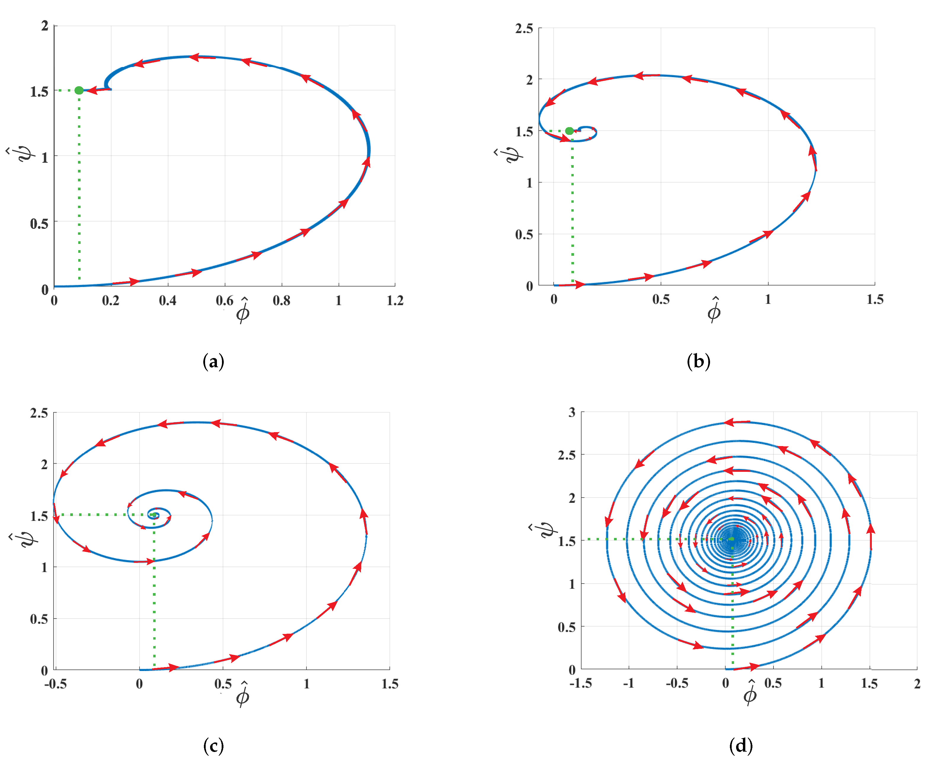
On the other hand, we employ the phase portrait approach to represent the Buck-Boost converter dynamic in the phase plane geometrically. The main idea is to identify those equilibrium points permitting the system to maintain stable states. Retracing the path of the fractional calculus concept applied to this work, the phase portraits shown in Figure 8 considered null initial conditions with different $\alpha$ values.

Figure 8. Phase portrait of the fractional-order Buck-Boost converter at different values of $\alpha$: (a) $\alpha =0.7$, (b) $\alpha =0.8$, (c) $\alpha =0.9$, (d) $\alpha =1$.

Analyzing the obtained phase portraits, one can see that the equilibrium point $(1.54,0.2)$ remains constant for all $\alpha$ values. Furthermore, we detected two significant findings regarding the $\alpha$ range. The first one liaises a low $\alpha$ value so that the trajectory toward the equilibrium point is much faster and more stable than in the other cases (cf. Figure 8a). The second one corresponds to the unit value of $\alpha$, which leads to an asymptotically stable spiral point (cf. Figure 8d). With this in mind, the obtained results prove that a fractional-order Buck-Boost model yields an improved behavior and performance than an integer-order model.

5. Conclusions

In general terms, most DC–DC converters adopt the integer-order approach for representing the behavior of their electrical components. Consequently, the mathematical models of such converters do not match the reported experimental data. Therefore, the proposed fractional-order Buck-Boost converter model was nondimensionalized, and the fractional-order state–space model was deduced to avoid integer-order model inconsistencies in the analysis. To carry this out, the inductor current and capacitor voltage were determined through the fractional Riemann–Liouville definition in the stable state. Moreover, the steady-state response of the system showed variations while the order of the derivative changed. Some models demonstrated a remarkable performance over the integer-order model. This phenomenon happened for $\alpha$ values of $0.7$. Therefore, we consider that decreasing below this value makes building the model very difficult. The proposed nondimensionalized model was tested using the Simulink and FOMCOM. It is worth mentioning that the parameter $\alpha$ directly impacts the capacitor voltage and inductor current responses. Additionally, we determined that the converter reaches the desired behavior when $\alpha =0.7$. According to the obtained results, the fractional-order concept used in this work seems feasible for achieving more realistic models of DC–DC converters. Finally, the experimental tests led to the design of a Buck-Boost converter with fractional-order electrical components that do not require complex control schemes.