Unscented Kalman Filter Empowered by Bayesian Model Evidence for System Identification in Structural Dynamics ^†

Abstract

System identification is often limited to parameter identification, while model uncertainties are disregarded or accounted for by a fictitious process noise. However, modelling assumptions may have a large impact on system identification. For this reason, we propose to use an unscented Kalman filter (UKF) empowered by online Bayesian model evidence computation for the sake of system identification and model selection. This approach employs more than one model to track the state of the system and associates with each model a plausibility measure, updated whenever new measurements are available. The filter outcomes obtained for different models are then compared and a quantitative confidence value is associated with each of them. Only the system identification outcomes related to the model with the highest plausibility are considered. While the coupling of extended Kalman filters (EKFs) and Bayesian model evidence was already addressed, we modify the approach to exploit the most striking features of the UKF, namely, the ease of implementation and higher-order accuracy in the description of the evolution of the state mean and variance. A challenging identification problem related to structural dynamics is discussed to show the effectiveness of the proposed methodology.

1. Introduction

Kalman filters (KFs) are well-known tools for system identification. They work by applying a predictor phase, in which a suitable model is needed to predict the evolution of a dynamic system, and a correction phase, in which corrections to the prediction are applied by recursively processing system measurements [1].

In civil and mechanical engineering, different model classes, consisting of different parametrizations of the structure to be identified, can be formulated. They are built upon different levels of complexity in the description of the system mechanics and uncertainty in the formulation of the modelling assumptions. Emphasis is usually placed on improving the quality of the parameter estimate, especially whenever nonlinear dynamic systems are handled. With this goal, KF extensions such as the extended Kalman filter (EKF) or the unscented Kalman filter (UKF) have been introduced. On the contrary, model uncertainties are often disregarded or accounted for by a fictitious process noise. In this work, we propose a way to tackle this aspect by calculating a quantitative estimate, referred to as model evidence, measuring how much the model employed by the KF is plausible with respect to other possible parametrizations. While a similar estimate was discussed in [2] for the EKF, here, we develop a model evidence formula suited for the UKF to exploit its ease of implementation and higher-order accuracy in the description of the evolution of the state mean and variance.

The remainder of the contribution is organized as follows: In Section 2, first, the governing equations of a mechanical elasto-dynamic system are discussed; second, the related algorithm showing the application of the UKF for parameter estimation is reported and finally, the equations allowing for recursive model evidence calculation are presented. In Section 3, a case study featuring a shear building excited by real ground acceleration is discussed, showing how parameter identification outcomes are affected by different structural parametrizations and how model evidence can be used for the sake of model selection a posteriori. Conclusions are finally discussed in Section 4.

2. Methodology

2.1. Elasto-Dynamic Problem

We focus on situations where the system dynamics is described by the finite element (FE) discretised version of a general elasto-dynamic problem. At time $t_{k+1}$, it reads:

$$\mathbf{M}{\ddot{\mathbf{q}}}_{k+1}+\mathbf{C}{\dot{\mathbf{q}}}_{k+1}+\mathbf{K}{\mathbf{q}}_{k+1}={\mathbf{f}}_{k+1},k=0,\dots ,n_{t-1}$$

(1)

where $\mathbf{M}$, $\mathbf{C}$ and $\mathbf{K}$ are the mass, damping and stiffness matrices, respectively; $\mathbf{q},\dot{\mathbf{q}},\ddot{\mathbf{q}}\in {\mathbb{R}}^{n\times 1}$ are the nodal displacements, velocities and accelerations, respectively; and ${\mathbf{f}}_{k+1}\in {\mathbb{R}}^{n\times 1}$ is the external force vector, assumed to be known.

Equation (1) is integrated in time by using the $\alpha$-method [3], ruled by the parameters ${\alpha }_m$, ${\alpha }_f$ and $\beta$. At each time step, the displacement field ${\mathbf{q}}_{k+1}$ is obtained by solving

$${\mathbf{K}}_{k+1}^{*}{\mathbf{q}}_{k+1}={\mathbf{f}}_{k+1}^{*}\left({\mathbf{q}}_k,{\dot{\mathbf{q}}}_k,{\ddot{\mathbf{q}}}_k\right).$$

(2)

The modified matrix ${\mathbf{K}}^{*}$ and the right hand side vector ${\mathbf{f}}_{k+1}^{*}$ are computed by

$${\mathbf{K}}_{k+1}^{*}=\frac{1-{\alpha }_m}{\beta \Delta t^2}\mathbf{M}+\frac{\gamma \left(1-{\alpha }_f\right)}{\beta \Delta t}\mathbf{C}+\left(1-{\alpha }_f\right)\mathbf{K},$$

(3)

$$\begin{array}{c}\hfill {\mathbf{f}}_{k+1}^{*}\left({\mathbf{q}}_k,{\dot{\mathbf{q}}}_k,{\ddot{\mathbf{q}}}_k\right)={\mathbf{f}}_{k+1-{\alpha }_f}+\left(\frac{1-{\alpha }_m}{\beta \Delta t^2}\left({\mathbf{q}}_k+\Delta t\dot{{\mathbf{q}}_k}\right)+\frac{1+{\alpha }_m-2\beta }{2\beta }{\ddot{\mathbf{q}}}_k\right)\mathbf{M}+\\ \hfill \left(\frac{\gamma \left(1-{\alpha }_f\right)}{\beta \Delta t}{\mathbf{q}}_k-\frac{\beta -\gamma \left(1-{\alpha }_f\right)}{\beta }{\dot{\mathbf{q}}}_k-\left(1-\frac{\gamma }{2\beta }\right)\left(1-{\alpha }_f\right)\Delta t{\ddot{\mathbf{q}}}_k\right)\mathbf{C}-{\alpha }_f\mathbf{K},\end{array}$$

(4)

where $\Delta t=t_{k+1}-t_k$, $t_{k+1-{\alpha }_f}=\left(1-{\alpha }_f\right)t_{k+1}+{\alpha }_f{t}_k$, ${\mathbf{f}}_{k+1-{\alpha }_f}=\mathbf{f}\left(t_{k+1-{\alpha }_f}\right)$.

Moreover, the mechanical system is assumed to be only partially observed. Accordingly, a Boolean matrix $\mathbf{H}\in {\mathbb{R}}^{n_o\times 3n}$ establishes the connection between the $n_o$ observed quantities ${\widehat{\mathbf{y}}}_{k+1}\in {\mathbb{R}}^{n_o}$ and the kinematic fields, as follows:

$${\widehat{\mathbf{y}}}_{k+1}=\mathbf{H}{\left[{\mathbf{q}}_{k+1},{\dot{\mathbf{q}}}_{k+1},{\ddot{\mathbf{q}}}_{k+1}\right]}^T.$$

(5)

2.2. Unscented Kalman Filter for Parameter Estimation

In this study, the ultimate goal of filtering is to estimate the unknown parameters $\mathit{\theta }\in {\mathbb{R}}^{n_p\times 1}$ ruling the mechanical response of the structure to be identified, where typically $\mathbf{C}=\mathbf{C}\left(\mathit{\theta }\right)$ and $\mathbf{K}=\mathbf{K}\left(\mathit{\theta }\right)$. In [1,4], Kalman filtering techniques were successfully applied, even in the presence of nonlinearities due to damage evolution in the observed system, by solving a dual estimation problem and thereby adopting as state variables the model displacements and the unknown parameters governing the response of the mechanical domain. However, treating FE solutions characterized by a large number n of degrees of freedom (DOF) may result in an excessive computational burden when dealing with dual estimation. A possible solution consists of obtaining a reduced order model (ROM) representation of the mechanical domain and adopting as state variables, instead of the nodal kinematics, the ROM DOF [5,6]. This strategy has been explored in [7]. Here, we consider only $\mathit{\theta }$ as a state variable to avoid the computational burden connected to the combined use of UKF and DOF tracking when large FE models are addressed, despite the enhanced performance usually guaranteed by state tracking [1,8]. The following state-space representation is used:

$$\begin{array}{c}\hfill {\mathit{\theta }}_{k+1}={\mathit{\theta }}_k+{\mathbf{w}}_k\end{array}$$

(6a)

$$\begin{array}{c}\hfill {\mathbf{y}}_{k+1}={\widehat{\mathbf{y}}}_{k+1}+{\mathbf{v}}_{k+1}\end{array}$$

(6b)

where the $\mathit{\theta }$ is driven by a random walk ruled by ${\mathbf{w}}_k\in {\mathbb{R}}^{n_p\times 1}$, modelled as a white process noise ${\mathbf{w}}_k\sim \mathcal{N}\left(\mathbf{0},\mathbf{Q}\right)$, and the FE predicted output ${\widehat{\mathbf{y}}}_{k+1}$ is related to the actual response of the structure by adding a measurement noise ${\mathbf{v}}_{k+1}\in {\mathbb{R}}^{n_y\times 1}$, modelled as white ${\mathbf{v}}_{k+1}\sim \mathcal{N}\left(\mathbf{0},\mathbf{R}\right)$. The matrices $\mathbf{Q}$ and $\mathbf{R}$ are symmetric and positive defined. The time variation of $\mathit{\theta }$, introduced by the random walk formulation, is fictitious.

KFs attempt to propagate the mean and the covariance of the state variable vector through the state-space and the measurement update equations. Instead of propagating the probability density functions associated with the state variables, it is indeed preferable to draw a set of samples, deterministically propagate them and finally compute the mean and covariance of the state vector; this is especially profitable when the state-space and/or the measurement update equations are nonlinear. The UKF is based on this idea. The propagated vector collects a set of so-called sigma points (SPs) ${\mathit{\vartheta }}_k^i$, $i=1,\dots ,\left(2n_{\theta }+1\right)$, distributed such that the mean and covariance of these points match those of the state variables. A scaled version of the UKF is used by setting the parameters ${\alpha }_{SP}$, ${\kappa }_{SP}$ and ${\beta }_{SP}$, as detailed in [9], to avoid sampling nonlocal effects that would spoil the state variable mean and covariance reconstruction [10]. In the predictor phase, this vector is propagated from the k-th to the k+1-th time step through the state-space equations. In the corrector phase, the estimated output covariance ${\widehat{\mathbf{P}}}_{k+1|k}^{yy}$ and the estimated cross covariance ${\widehat{\mathbf{P}}}_{k+1|k}^{\theta y}$ are used to compute the Kalman gain ${\mathbf{G}}_{k+1}$ needed to correct the propagated mean ${\widehat{\mathit{\theta }}}_{k+1|k}$ and covariance ${\widehat{\mathbf{P}}}_{k+1|k}^{\theta \theta }$ on the basis of the collected measurements ${\mathbf{y}}_{k+1}$. The full expression of these quantities and the application of the UKF are detailed in Algorithm 1, adapted from [11].

2.3. Model Evidence Computation for Unscented Kalman Filter

System identification is usually limited to select a particular parametric model $\mathcal{M}$ of the underlying structural system, estimating the corresponding unknown parameters $\mathit{\theta }$. However, the use of either excessively simplified or too complex models may have a detrimental effect on the possibility to track the system state: oversimplified models may underestimate the effect of a physical process taking place; on the other hand, complex models may lead to good data fitting but possibly yield to poor predictions. In the latter case, the model overfits the incoming data. In [2], an online model class selection strategy was proposed in the framework of an EKF’s parameter estimates. Here, a similar approach was adopted for a simultaneous parametric estimate and model class selection exploiting the UKF. Adopting a number $n_m$ of possible model classes, the model evidence (or plausibility) consisting of the probability $p\left({\mathcal{M}}_{k+1}^m\right)\in \left(0,1\right)$ was computed for each model class ${\mathcal{M}}^m$, with $m=1,\dots ,n_m$ at each time step $t_{k+1}$. The sum of the $n_m$ model evidences is equal to the unity. To derive the expression of $p\left({\mathcal{M}}_{k+1}^m\right)$, first, the Bayes theorem was used, giving

$$p\left({\mathcal{M}}_{k+1}^m\right)=\frac{p\left({\mathbf{y}}_{k+1}|{\mathcal{M}}_k^m\right)p\left({\mathcal{M}}_k^m\right)}{{\displaystyle \sum _{l=1}^{n_m}}p\left({\mathbf{y}}_{k+1}|{\mathcal{M}}_k^l\right)p\left({\mathcal{M}}_k^l\right)},$$

(7)

where $p\left({\mathbf{y}}_{k+1}|{\mathcal{M}}_k^m\right)$, called conditional evidence, represents the contribution of the measurement at $t_{k+1}$ to the plausibility of the m-th model class.

Second, we extended the procedure explained in [2] from the EKF to the UKF. As a result, at the end of the corrector phase (after Step 15 of Algorithm 1), the following expression for the conditional evidence applied:

$$\begin{array}{c}\hfill p\left({\mathbf{y}}_{k+1}|\widehat{\mathit{\theta }},{\mathcal{M}}_k^m\right)\approx {\left(2\pi \right)}^{-\frac{n_o}{2}}{\left[\det \left({\widehat{\mathbf{P}}}_{k+1|k+1}^{\theta \theta }{\left({\widehat{\mathbf{P}}}_{k+1|k}^{\theta \theta }\right)}^{-1}\right)\right]}^{\frac{1}{2}}{\left[\det \left({\widehat{\mathbf{P}}}_{k+1|k}^{yy}{}^{-1}\right)\right]}^{\frac{1}{2}}\\ \hfill \times \exp [-\frac{1}{2}{\left({\widehat{\mathit{\theta }}}_{k+1|k+1}-{\widehat{\mathit{\theta }}}_{k+1|k}\right)}^T{\left({\widehat{\mathbf{P}}}_{k+1|k}^{\theta \theta }\right)}^{-1}\left({\widehat{\mathit{\theta }}}_{k+1|k+1}-{\widehat{\mathit{\theta }}}_{k+1|k}\right)\\ \hfill -\frac{1}{2}{\left({\mathbf{y}}_{1:k+1}-{\widehat{\mathbf{y}}}_{1:k+1|k}\right)}^T{\left({\widehat{\mathbf{P}}}_{k+1|k}^{yy}\right)}^{-1}\left({\mathbf{y}}_{1:k+1}-{\widehat{\mathbf{y}}}_{1:k+1|k}\right)],\end{array}$$

(8)

where $\det \left(·\right)$ calculates the determinant of the input matrix. The reported expression approximates $p\left({\mathbf{y}}_{k+1}|\widehat{\mathit{\theta }},{\mathcal{M}}_k^m\right)$ due to the use of Laplace’s asymptotic expansion [2].

Algorithm 1 UKF for parameter estimation, linear elastic case.

1: for $k=0,\dots ,n_t$                       ▹ loop over the time steps $$\mathrm{Predictor}\mathrm{phase}$$ 2: Assume ${\widehat{\mathit{\theta }}}_{k+1|k}={\widehat{\mathit{\theta }}}_{k|k}$, according to Equation (6a)     ▹ prior estimate of the state variables 3: Assume ${\widehat{\mathbf{P}}}_{k+1|k}^{\theta \theta }={\widehat{\mathbf{P}}}_{k|k}^{\theta \theta }+\mathbf{Q}$         ▹ prior covariance of the state variable estimate 4: Generate ${\mathit{\vartheta }}_{k+1}^i$, $i=1,\dots ,(2n_{\mathit{\theta }}+1)$, using ${\widehat{\mathit{\theta }}}_{k+1|k}$ and ${\widehat{\mathbf{P}}}_{k+1|k}^{\theta \theta }$ as in [9]                                         ▹ SPs 5: Compute ${\mathbf{q}}_{k+1}^i={\left({\mathbf{K}}_{k+1}^{*i}\left({\mathit{\vartheta }}_{k+1}^i\right)\right)}^{-1}{\mathbf{f}}_{k+1}^i\left({\mathbf{q}}_k,{\dot{\mathbf{q}}}_k,{\ddot{\mathbf{q}}}_k,{\mathit{\vartheta }}_{k+1}^i\right)$▹ displacement field for each SP 6: Compute ${\dot{\mathbf{q}}}_{k+1}^i$ and ${\ddot{\mathbf{q}}}_{k+1}^i$             ▹ velocity and acceleration fields for each SP 7: Compute ${\mathfrak{y}}_{k+1}^i=\mathbf{H}{\left[{\mathbf{q}}_{k+1}^i,{\dot{\mathbf{q}}}_{k+1}^i,{\ddot{\mathbf{q}}}_{k+1}^i\right]}^T$          ▹ system observation for each SP 8: Compute ${\widehat{\mathbf{y}}}_{k+1|k}={\sum }_{i=1}^{2n_{\theta }+1}{w}_m^i{\mathfrak{y}}_{k+1}^i$                   ▹ predicted output $$\mathrm{Corrector}\mathrm{phase}$$ 9: Compute ${\widehat{\mathbf{P}}}_{k+1|k}^{yy}={\sum }_{i=1}^{2n_{\theta }+1}{w}_c^i\left[{\mathfrak{y}}_{k+1}^i-{\widehat{\mathbf{y}}}_{k+1|k}\right]{\left[{\mathfrak{y}}_{k+1}^i-{\widehat{\mathbf{y}}}_{k+1|k}\right]}^T+\mathbf{R}$                              ▹ estimated output covariance 10: Compute ${\widehat{\mathbf{P}}}_{k+1|k}^{\theta y}={\sum }_{i=1}^{2n_{\theta }+1}{w}_c^i\left[{\mathit{\vartheta }}_{k+1}^i-{\widehat{\mathit{\theta }}}_{k+1|k}\right]{\left[{\mathfrak{y}}_{1:k+1}^i-{\widehat{\mathbf{y}}}_{1:k+1|k}\right]}^T$                              ▹ estimated cross covariance 11: Compute ${\mathbf{G}}_{k+1}={\widehat{\mathbf{P}}}_{k+1|k}^{\theta y}{\left({\widehat{\mathbf{P}}}_{k+1|k}^{yy}\right)}^{-1}$                   ▹ Kalman gain 12: Update the prior estimate ${\widehat{\mathit{\theta }}}_{k+1|k+1}={\widehat{\mathit{\theta }}}_{k+1|k}+{\mathbf{G}}_{k+1}\left({\mathbf{y}}_{k+1}-{\widehat{\mathbf{y}}}_{k+1|k}\right)$                         ▹ posterior estimate of the state variables 13: Update the prior estimate ${\widehat{\mathbf{P}}}_{k+1|k+1}^{\theta \theta }={\widehat{\mathbf{P}}}_{k+1|k}^{\theta \theta }-{\mathbf{G}}_{k+1}{\widehat{\mathbf{P}}}_{k+1|k}^{yy}{\mathbf{G}}_{k+1}^T$                    ▹ posterior covariance of the state variable estimate 14: Compute ${\mathbf{q}}_{k+1}={\left({\mathbf{K}}_{k+1}^{*}\left({\widehat{\mathit{\theta }}}_{k+1|k+1}\right)\right)}^{-1}{\mathbf{rhs}}_{k+1}\left({\mathbf{q}}_k,{\dot{\mathbf{q}}}_k,{\ddot{\mathbf{q}}}_k,{\widehat{\mathit{\theta }}}_{k+1|k+1}\right)$                                  ▹ displacement field 15: Compute ${\dot{\mathbf{q}}}_{k+1}$ and ${\ddot{\mathbf{q}}}_{k+1}$                 ▹ velocity and acceleration fields 16: end for

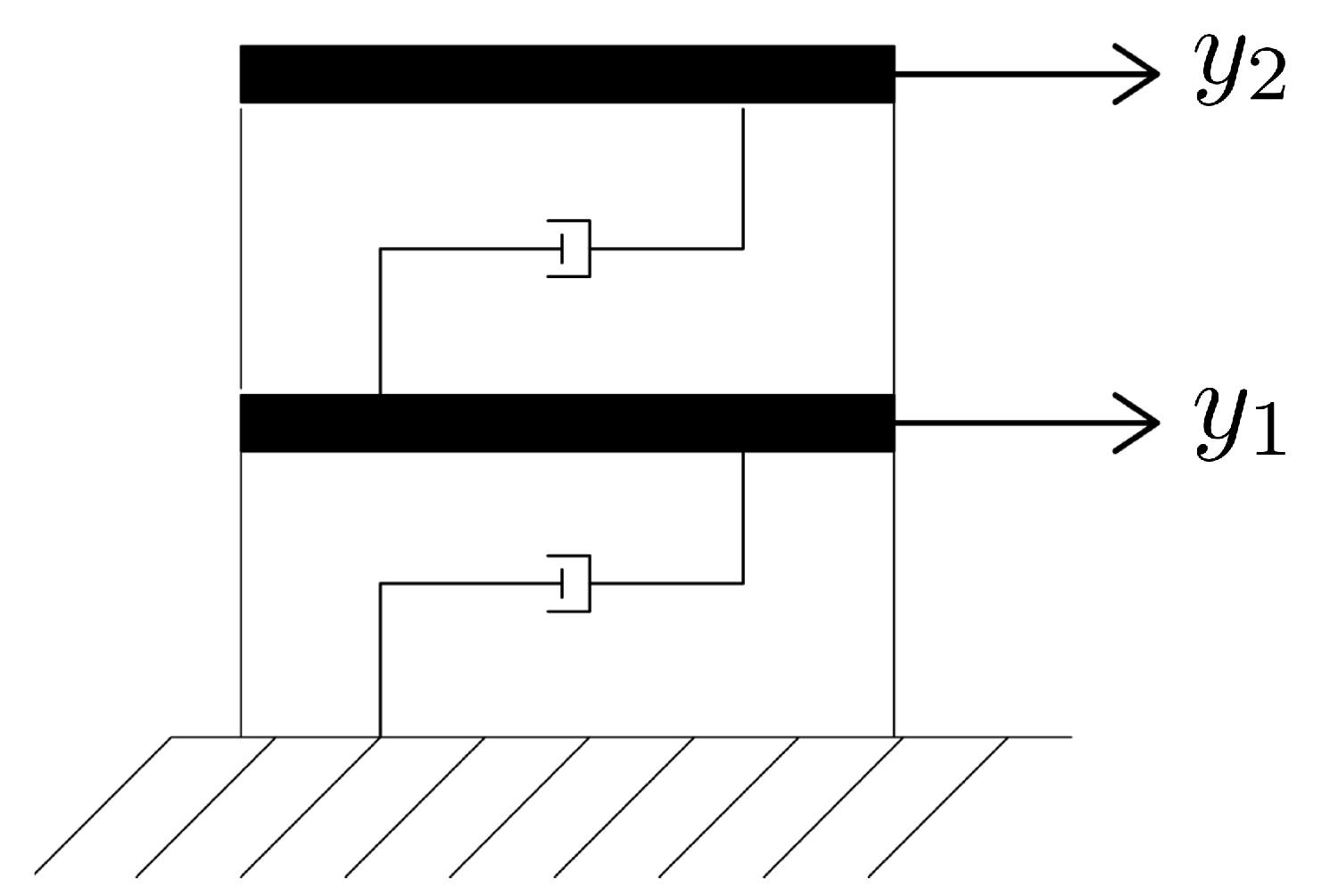
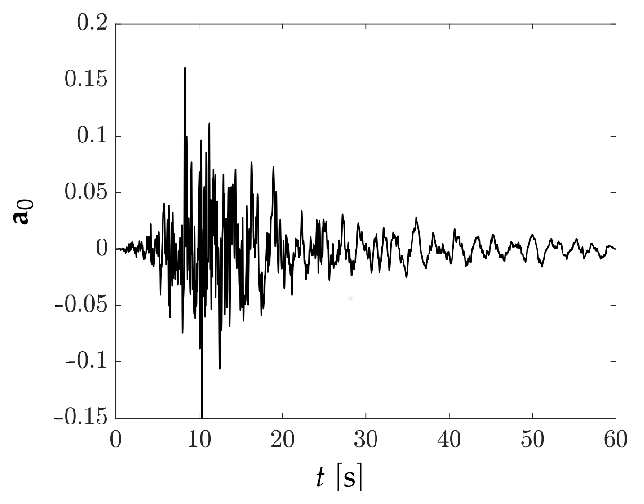
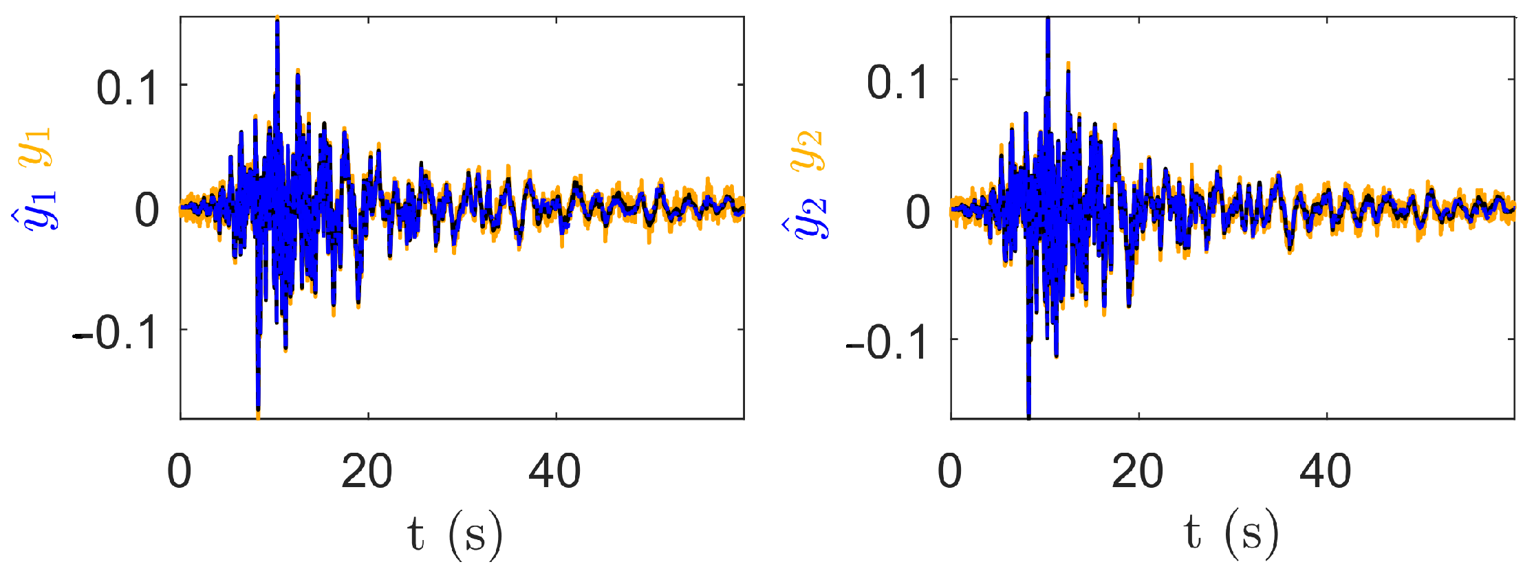
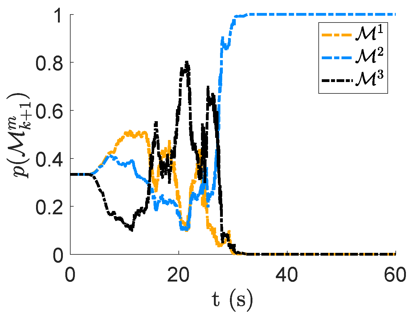
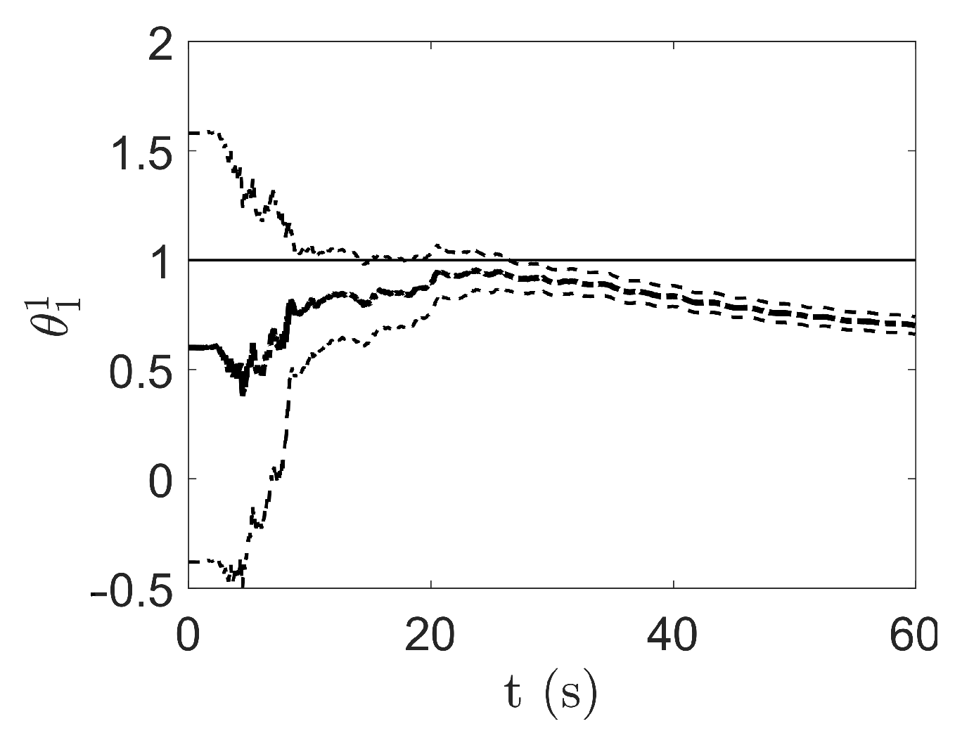
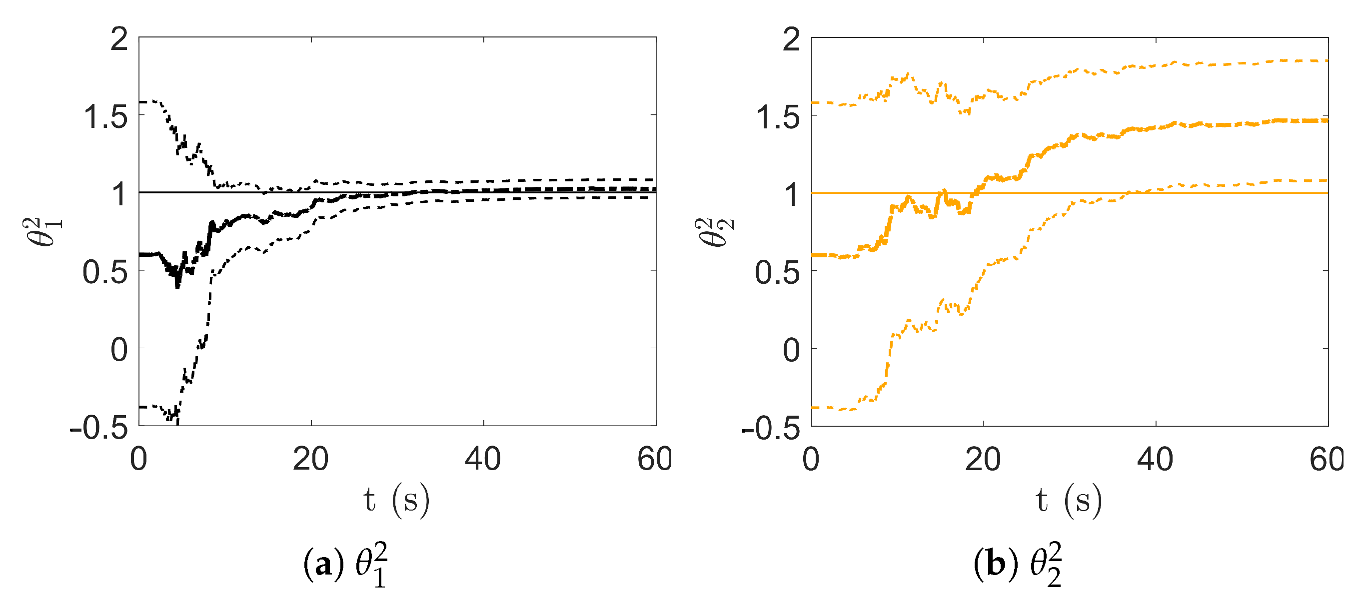
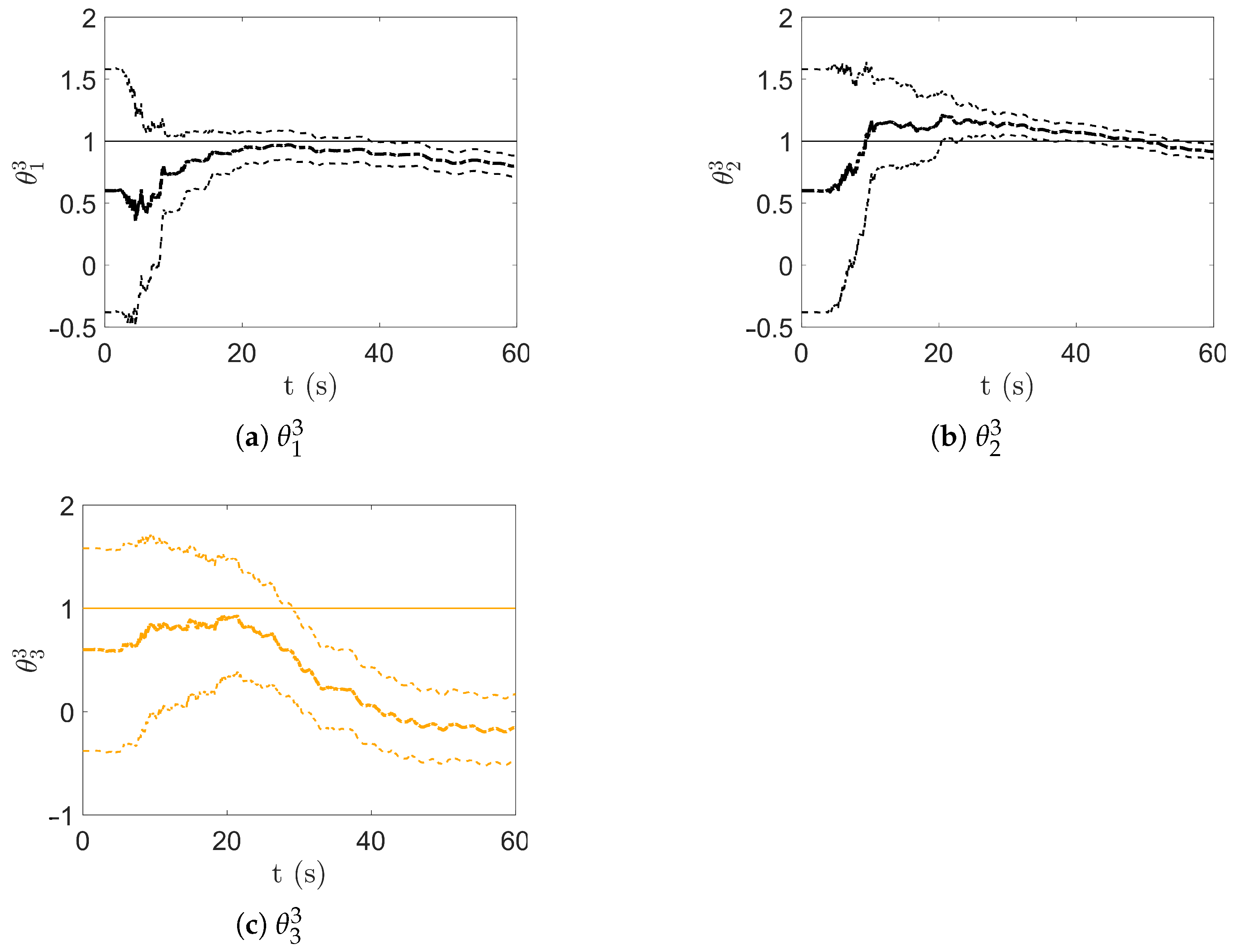
3. Results and Discussion

As a numerical case study, we studied how to determine the interstorey stiffness and damping of the two DOF shear building models ($n=2$) reported in Figure 1. The mechanical properties of the building were adimensionalised to ease the UKF tuning by setting the matrices in Equation (1) equal to

$$\mathbf{M}=\left[\begin{array}{cc}2& 0\\ 0& 2\end{array}\right],\mathbf{C}=\left[\begin{array}{cc}0.2& -0.1\\ -0.1& 0.1\end{array}\right],\mathbf{K}=\left[\begin{array}{cc}2& -1\\ -1& 1\end{array}\right].$$

Figure 1. Two DOF shear model. Acceleration monitoring.

The building was excited by the ground acceleration ${\mathbf{a}}_0$ reported in Figure 2, lasting $60\mathrm{s}$. The response of the building was monitored by recording the floor acceleration $\mathbf{y}={\left[y_1,y_2\right]}^T$ with a sampling frequency of $50\mathrm{Hz}$ for a total of $n_t=3000$ samples. A white noise, featuring a standard deviation of $5\times {10}^{-3}$, was added to $y_1$ and to $y_2$ to mimic the signal perturbation affecting micro-electro-mechanical accelerometers [12].

Figure 2. Ground acceleration.

The acceleration recordings coming from this reference building were used as measurements in the corrector phase of the filtering procedure (Steps 9 and 10 of Algorithm 1). Three model classes, ${\mathcal{M}}^1$, ${\mathcal{M}}^2$ and ${\mathcal{M}}^3$, featuring different structural parametrizations, were considered, as shown in the following:

$${\mathbf{C}}^1=\left[\begin{array}{cc}0.12& -0.06\\ -0.06& 0.06\end{array}\right],{\mathbf{K}}^1\left({\theta }_1^1\right)={\theta }_1^1\left[\begin{array}{cc}2& -1\\ -1& 1\end{array}\right]$$

$${\mathbf{C}}^2\left({\theta }_2^2\right)={\theta }_2^2\left[\begin{array}{cc}0.2& -0.1\\ -0.1& 0.1\end{array}\right],{\mathbf{K}}^2\left({\theta }_1^2\right)={\theta }_1^2\left[\begin{array}{cc}2& -1\\ -1& 1\end{array}\right]$$

$${\mathbf{C}}^3\left({\theta }_3^3\right)={\theta }_3^3\left[\begin{array}{cc}0.2& -0.1\\ -0.1& 0.1\end{array}\right],{\mathbf{K}}^3\left({\theta }_1^3,{\theta }_2^3\right)=\left[\begin{array}{cc}{\theta }_1^3{\theta }_2^3& -{\theta }_2^3\\ -{\theta }_2^3& {\theta }_2^3\end{array}\right].$$

Model class ${\mathcal{M}}^1$ is governed by the parameter ${\theta }_1^1$ ruling the interstorey stiffness of both floors (for this reason, ${\theta }_1^1$ is factored out from ${\mathbf{K}}^1$); ${\mathcal{M}}^2$ is governed by ${\theta }^2={\left[{\theta }_1^2,{\theta }_2^2\right]}^T$ ruling, respectively, the interstorey stiffness and damping of both floors; ${\mathcal{M}}^3$ is governed by ${\theta }^3={\left[{\theta }_1^3,{\theta }_2^3,{\theta }_3^3\right]}^T$, where ${\theta }_1^3$ and ${\theta }_2^3$ rule the first and second floor interstorey stiffness and ${\theta }_3^3$ rules the damping associated with both floors. Comparing these parametrizations with the reference model, it is clear that ${\mathcal{M}}^1$ is underparametrizing the mechanical system, not associating any parameter with the damping properties of the structures and suffering a model bias, being ${\mathbf{C}}^1=0.6\mathbf{C}$; ${\mathcal{M}}^3$ is overparametrizing the stiffness matrix and ${\mathcal{M}}^2$ is performing a correct parametrization of the structural response, and it is therefore expected to allow for the best estimate of the system mechanical properties. For all model classes, the initial guesses of the relevant parameters underestimated by $40\%$ of the parameter values ruling the reference structure.

KF tuning is usually problem-dependent and is performed through a trial-and-error procedure. In this case, we have set the SP scaling parameters to ${\alpha }_{SP}={10}^{-3}$, ${\kappa }_{SP}=0$ and ${\beta }_{SP}=2$; the measurement noise covariance to $\mathbf{R}=4\times {10}^{-4}{\mathbf{I}}_2$, where ${\mathbf{I}}_2\in {\mathbb{R}}^{2\times 2}$ is the identity matrix; the process noise covariance to $\mathbf{Q}={10}^{-8}{\mathbf{I}}_{n_p}$, with ${\mathbf{I}}_{n_p}\in {\mathbb{R}}^{n_p\times n_p}$; and the initial parameter covariance to ${\widehat{\mathbf{P}}}_0^{\theta \theta }=0.25{\mathbf{I}}_{n_p}$. The value of $n_p$ depends on the number of parameters employed by each model ($n_p=1$ for ${\mathcal{M}}^1$, $n_p=2$ for ${\mathcal{M}}^2$ and $n_p=3$ for ${\mathcal{M}}^3$).

In Figure 3, the predicted output of ${\mathcal{M}}^1$, computed according to Step 8 of Algorithm 1, is reported against the floor acceleration measurements, showing the filter capacity of tracking the shear building accelerations despite the presence of noise. A small discrepancy between the reference model and the predicted output is observable only magnifying the curves. The predicted outputs of ${\mathcal{M}}^2$ and ${\mathcal{M}}^3$, not reported for lack of space, exhibit an even smaller discrepancies.

Figure 3. ${\mathcal{M}}^1$ predicted outputs (dot dashed blue line) are reported against the noise-corrupted reference model recordings (orange line). The left figure refers to the first floor and the right figure to the second floor. Black lines depict the reference model acceleration when not corrupted by noise.

The filter capacity of tracking the system output was expected to greatly help parameter identification. In Figure 4, Figure 5 and Figure 6, the time evolution of the parameters employed by ${\mathcal{M}}^1$, ${\mathcal{M}}^2$ and ${\mathcal{M}}^3$ are reported, respectively. Black colour is used for parameters involved in the expression of the structural stiffness; orange colour when related to the structural damping. The plots report both the parameter posterior estimates and the confidence intervals of these estimates. Looking at the confidence intervals, stiffness-related parameters seem to assume negative values during the first part of the analyses. This is due to to the initial choice of ${\widehat{\mathbf{P}}}_0^{\theta \theta }=0.25{\mathbf{I}}_{n_p}$. However, positive values have been always associated with the interstorey stiffness due to the use of the scaled version of the UKF. Similar reasoning applies to damping-related parameters.

Figure 4. Model class ${\mathcal{M}}^1$, time evolution of ${\mathit{\theta }}_1^1$. The thicker dotted line reports the posterior estimate; the thinner dotted lines the $99\%$ confidence interval of the estimate, determined using the posterior covariance. The continuous line reports the parameter value assumed by the reference model.

Figure 5. Model class ${\mathcal{M}}^2$, time evolution of ${\mathit{\theta }}^2$. The thicker dotted line reports the posterior estimate; the thinner dotted line the $99\%$ confidence interval of the estimate, determined using the posterior covariance. The continuous line reports the parameter values assumed by the reference model.

Figure 6. Model class ${\mathcal{M}}^3$, time evolution of ${\theta }^3$. The thicker continuous line reports the posterior estimates; the thinner dotted lines the $99\%$ confidence interval of the estimate, determined using the posterior covariance. The continuous line reports the parameter values assumed by the reference model.

Looking at Figure 4, the UKF was unable to provide a correct estimate for ${\theta }_1^1$, despite the uncertainty reduction linked to the narrowing of the confidence interval. Even the stiffness-related parameters ${\theta }_1^3$ and ${\theta }_2^3$ of ${\mathcal{M}}^3$, depicted in Figure 6, seem not able to converge to the desired value. On the contrary, coming to ${\mathcal{M}}^2$, ${\theta }_1^2$ was correctly identified with small uncertainty, as shown in Figure 5. These results were somehow expected due to the underparametrization of the mechanical system operated by ${\mathcal{M}}^1$ and the overparametrization of the mechanical system exhibited by ${\mathcal{M}}^3$, while ${\mathcal{M}}^2$ embodied the correct description of the reference model.

Model class ${\mathcal{M}}^3$ was unable to provide any idea of the damping properties, ending up pushing ${\theta }_3^3$ to 0. Model class ${\mathcal{M}}^2$ provided a better estimate, still quite poor, overestimating by $40\%$ the damping related parameter ${\theta }_2^2$. These difficulties were due to the relevance of damping in the identification of continuously excited structures, discussed in [4].

From the results reported above, ${\mathcal{M}}^2$ seems to lead to the best system identification; however, we reached this conclusion by knowing the mechanical properties of the reference system. It would have been very hard, if not impossible, to judge model plausibility simply looking at the predicted outputs. Indeed, as shown in Figure 3, the UKF has been able to reproduce the monitoring system outcome even when ${\mathcal{M}}^1$ is employed. For this reason, model evidence computation, whose outcome is reported in Figure 7, is extremely relevant to understand which model can be trusted the most.

Figure 7. Model evidence evolution of each model.

At the beginning of the identification procedure, equal plausibility was associated with the three models. Their values were recursively updated as soon as new measurements became available using Equations (7) and (8). During the first part of the analysis, ${\mathcal{M}}^1$ appeared to be the most plausible model class. This is in agreement with intuition: ${\mathcal{M}}^1$ is the easiest to tune, employing just one parameter, and the bias in the modelling of damping has a marginal relevance when $t<20\mathrm{s}$ due to the strong ground motion undergone by the structure. In a second stage, ${\mathcal{M}}^3$ resulted to be the most plausible model class. This was due to the good estimate of both the stiffness-related parameters and the damping-related parameters in the central part of the analysis. Finally, the overcomplexity of ${\mathcal{M}}^3$ led to a deterioration of the parameter identification, while the good convergence of the stiffness-related parameters and the reasonable damping estimate promoted ${\mathcal{M}}^2$ as the most plausible model class.

This numerical example shows that model evidence evaluation can be successfully used for model selection. The reader should note that, due to the recursive nature of Equation (7), a certain time delay occurred between the improved identification capacity of the filter equipped with a certain model and the increase in plausibility of this model.

4. Conclusions

In this work, we have discussed an algorithm for simultaneous parameter estimation and model evidence calculation in dynamic linear elastic problems. Starting from the work of [2], a recursive expression for model evidence evaluation was derived for when the unscented Kalman filter is used. Numerical results show that model evidence can guide system identification in the presence of model uncertainties by associating a plausibility measure with different employed models featuring possible parametrizations of mechanical domains. Indeed, model evidence can be successfully used to select the most plausible structure parametrization as parameter identification is carried out.

References

- Mariani, S.; Ghisi, A. Unscented Kalman filtering for nonlinear structural dynamics. Nonlinear Dyn. 2007, 49, 131–150. [Google Scholar] [CrossRef]
- Yuen, K.V.; Mu, H.Q. Real-time system identification: an algorithm for simultaneous model class selection and parametric identification. Comput.-Aided Civ. Infrastruct. Eng. 2015, 30, 785–801. [Google Scholar] [CrossRef]
- Hilber, H.M.; Hughes, T.J.R.; Taylor, R.L. Improved numerical dissipation for time integration algorithms in structural dynamics. Earthq. Eng. Struct. Dyn. 1977, 5, 283–292. [Google Scholar] [CrossRef] [Green Version]
- Mariani, S.; Corigliano, A. Impact induced composite delamination: state and parameter identification via joint and dual extended Kalman filters. Comput. Methods Appl. Mech. Eng. 2005, 194, 5242–5272. [Google Scholar] [CrossRef]
- Eftekhar Azam, S.; Mariani, S.; Attari, N.K.A. Online damage detection via a synergy of proper orthogonal decomposition and recursive Bayesian filters. Nonlinear Dyn. 2017, 89, 1489–1511. [Google Scholar] [CrossRef]
- Eftekhar Azam, S.; Mariani, S. Online damage detection in structural systems via dynamic inverse analysis: A recursive Bayesian approach. Eng. Struct. 2018, 159, 28–45. [Google Scholar] [CrossRef]
- Gobat, G.; Azam, S.E.; Mariani, S. SHM and efficient strategies for reduced-order modeling. Eng. Proc. 2020, 2, 2098. [Google Scholar] [CrossRef]
- Kopp, R.E.; Orforf, R.J. Linear regression applied to system identification for adaptive control systems. AIAA J. 1963, 1, 2300–2306. [Google Scholar] [CrossRef]
- Wan, E.; Van Der Merwe, R. The unscented Kalman filter for nonlinear estimation. In Proceedings of the IEEE 2000 Adaptive Systems for Signal Processing, Communications, and Control Symposium (Cat. No.00EX373), Lake Louise, AL, Canada, 1–4 October 2000; pp. 153–158. [Google Scholar] [CrossRef]
- Julier, S. The scaled unscented transformation. In Proceedings of the 2002 American Control Conference (IEEE Cat. No.CH37301), Anchorage, AK, USA, 8–10 May 2002; Volume 6, pp. 4555–4559. [Google Scholar] [CrossRef] [Green Version]
- Castiglione, J.; Astroza, R.; Eftekhar Azam, S.; Linzell, D. Auto-regressive model based input and parameter estimation for nonlinear finite element models. Mech. Syst. Signal Process. 2020, 143, 106779. [Google Scholar] [CrossRef]
- D’Alessandro, A.; Vitale, G.; Scudero, S.; D’Anna, R.; Costanza, A.; Fagiolini, A.; Greco, L. Characterization of MEMS accelerometer self-noise by means of PSD and Allan Variance analysis. In Proceedings of the 7th IEEE International Workshop on Advances in Sensors and Interfaces IWASI, Vieste, Italy, 15–17 June 2017; pp. 159–164. [Google Scholar]
Publisher’s Note: MDPI stays neutral with regard to jurisdictional claims in published maps and institutional affiliations. |
© 2021 by the authors. Licensee MDPI, Basel, Switzerland. This article is an open access article distributed under the terms and conditions of the Creative Commons Attribution (CC BY) license (https://creativecommons.org/licenses/by/4.0/).