A Bicriteria Model for Saving a Path Minimizing the Time Horizon of a Dynamic Contraflow ^†

Abstract

The quickest contraflow in a single-source-single-sink network is a dynamic flow that minimizes the time horizon of a given flow value at the source to be sent to the sink allowing arc reversals. Because of the arc reversals, for a sufficiently large value of the flow, the residual capacity of all or most of the paths towards the source, from a given node, may be zero or reduced significantly. In some cases, e.g., for the movement of facilities to support an evacuation in an emergency, it is imperative to save a path from a given node towards the source. We formulate such a problem as a bicriteria optimization problem, in which one objective minimizes the length of the path to be saved from a specific node towards the source, and the other minimizes the quickest time of the flow from the source towards the sink, allowing arc reversals. We propose an algorithm based on the epsilon-constraint approach to find non-dominated solutions.

1. Introduction

Network flow modeling has been widely used for a variety of real-life applications. Because of their computational efficiency, they have been used to model problems involving significantly large networks. One of the important applications is evacuation planning, in which population in hazardous areas are shifted to safe areas using a complex urban road network. To use network flow modeling in such problems, a large urban road network is represented as a directed graph, and algorithms from graph theory and mathematical programming are used to identify the optimal traffic flow configuration. For a recent survey on evacuation planning problems, we refer to Dhamala et al. [1].

In evacuation planning problems, one of the important strategies is the contraflow approach, in which the appropriate direction of traffic is identified to optimize the flow, reversing the usual direction of traffic in the necessary road segments [2,3,4]. Recent research also focuses on location decisions along with flow decisions [5,6]. In contraflow planning, because of reversal of the direction of the traffic flow, the paths towards hazardous areas may be blocked. Sometimes, it is necessary to save a path towards such areas to transport necessary facilities. A path-saving strategy, with objectives to maximize the flow and minimize the length of the saved path is introduced in [7] as a bicriteria optimization model. In this paper, we extend the modeling to minimize the evacuation time and the length of the saved path. The paper is organized as follows. In Section 2, we give the basic ideas of network flow modeling. In Section 3, our main result, a bicriteria model to minimize the quickest time and the length of the saved path, is presented along with a solution algorithm. Section 4 concludes the paper.

2. Basic Ideas

A single-source-single-sink network $N=\left(V,A,s,t,u,\tau \right)$ is a directed graph with a set of nodes, $V$, and a set of arcs, $A\subseteq V\times V$. $s$ is a source node, $t$ is a sink node ($s\ne t$), $u:A\to {ℝ}_{\ge 0}$ assigns capacity $u_{ij}$, and $\tau :A\to {ℝ}_{\ge 0}$ assigns transit time ${\tau }_{ij}$ to the arcs of the network. For each $i\in V$, we define:

$$V_i^{+}=\left\{j\in V:\left(i,j\right)\in A\right\},$$

and

$$V_i^{-}=\left\{j\in V:\left(j, i\right)\in A\right\}.$$

2.1. Static Flow and Dynamic Flow

A static flow $x:A\to ℝ$ satisfies

$$0\le x_{ij}\le u_{ij}, \forall \left(i,j\right)\in A$$

(1)

and

$${\displaystyle \sum }_{j\in V_i^{+}}{x}_{ij}-{\displaystyle \sum }_{j\in V_i^{-}}{x}_{ji}=0, \forall i\in V\setminus \left\{s, t\right\}.$$

(2)

The value of $x$ is

$$v\left(x\right)={\displaystyle \sum }_{j\in V_s^{+}}{x}_{ij}-{\displaystyle \sum }_{j\in V_s^{-}}{x}_{ji}={\displaystyle \sum }_{j\in V_t^{-}}{x}_{ji}-{\displaystyle \sum }_{j\in V_t^{+}}{x}_{ij}.$$

(3)

If constraints (2) are satisfied for all $i\in V$, then $x$ is a circulation. If $P$ is a directed $s$–$t$ path, a chain flow $x^P$ is a static flow of value $\delta >0$ is defined by

$$x_{ij}^P=\{\begin{array}{cc}\delta & \left(i, j\right)\in P\\ 0& \mathrm{otherwise}\end{array}$$

(4)

If $C$ is a directed cycle, a cycle flow $x^C$ of value $\delta >0$ is a circulation defined by

$$x_{ij}^C=\{\begin{array}{cc}\delta & \left(i, j\right)\in C\\ 0& \mathrm{otherwise}\end{array}$$

(5)

A static flow $x$ can be decomposed into chain and cycle flows [8].

For a given time-horizon $T$, a dynamic flow $f={\left(f_{ij}\right)}_{\left(i,j\right)\in A}$ consists of Lebesgue measureable functions $f_{ij}:\left[0, T\right)\to {ℝ}_{\ge 0}$ such that $f_{ij}\left(\theta \right)=0$ for $\theta \ge T-{\tau }_{ij}$ and satisfies the following:

$$e_f\left(i,\theta \right)={\displaystyle \sum }_{j\in V_i^{-}}{f}_{ji}\left(\xi \right)d\xi -{\displaystyle \sum }_{j\in V_i^{+}}{f}_{ij}\left(\xi \right)d\xi \ge 0\hspace{1em}\forall i\in V\setminus \left\{s\right\}, \theta \in \left[0, T\right),$$

(6)

$$e_f\left(i,T\right)=0\hspace{1em}\forall i\in V\setminus \left\{s, t\right\},$$

(7)

$$0\le f_{ij}\left(\theta \right)\le u_{ij}\hspace{1em}\forall \left(i, j\right)\in A, \theta \in \left[0, T\right).$$

(8)

The value of $f$ is

$$v_T\left(f\right)=e_f\left(t,T\right).$$

(9)

Given a static flow, $x$, and a time horizon, $T$, a dynamic flow ($f$) can be obtained by sending a flow of value equal to that of $x^P$ along every path, $P$, repeating $T-\tau \left(P\right)$ times, in the chain-and-cycle decomposition of $x$. Such an $f$ is called a temporally repeated dynamic flow with the value

$$T v\left(x\right)-{\displaystyle \sum }_{\left(i,j\right)\in A}{x}_{ij}{\tau }_{ij}$$

(10)

For more details, see [9,10].

Given a time horizon, a dynamic flow with maximum value is called a maximum dynamic flow. Given a supply ($Q$) assigned to the source, a dynamic flow of value $Q$ with a minimum time horizon is called a quickest flow.

According to [11], the static flow corresponding to the temporally repeated quickest flow can be found by solving a fractional programming problem with linear constraints.

Theorem 1.

(Lin and Jaillet [11]): The quickest flow problem can be formulated as the fractional programming problem:

$$\min \frac{Q+{{\displaystyle \sum }}_{\left(i, j\right)\in A}{\tau }_{ij}{x}_{ij}}{v}$$

(11)

subject to:

$${\displaystyle \sum }_{j\in V_i^{+}}{x}_{ij}-{\displaystyle \sum }_{j\in V_i^{-}}{x}_{ji}=\{\begin{array}{cc}\hfill v& \mathrm{for} i=s\hfill \\ \hfill -v& \mathrm{for} i=t\hfill \\ \hfill 0& \mathrm{for} i\in V\setminus \left\{s, t\right\}\hfill \end{array}$$

(12)

$$0\le x_{ij}\le u_{ij}, \forall \left(i, j\right)\in A$$

(13)

2.2. The Contraflow Problem

The problem of identification of optimal static (dynamic) flow with ideal direction of the arcs reversing the necessary arcs, is a static (dynamic) contraflow problem. In finding an analytical solution of the contraflow problems, an important strategy is to construct, what is known as, the auxiliary network from the given network. Let $N=\left(V, A, s, t, u,\tau \right)$ be a network with ${\tau }_{ij}={\tau }_{ji}$ whenever $\left(i, j\right), \left(j, i\right)\in A$. The auxiliary network $N^{\prime }=\left(V,A^{\prime },s,t,u^{\prime },{\tau }^{\prime }\right)$ is the network where $A^{\prime }$ consists of arcs $\left(i,j\right)$ and $\left(j, i\right)$ whenever $\left(i, j\right)$ or $\left(j, i\right)$ is in $A$. The capacity $u_{ij}^{\prime }=u_{ij}+u_{ji}$ with $u_{ij}=0$ whenever $\left(i, j\right)\notin A$, and the travel time ${\tau }_{ij}^{\prime }={\tau }_{ij}$ if $\left(i,j\right)\in A$, and ${\tau }_{ij}^{\prime }={\tau }_{ji}$ if $\left(j,i\right)\in A$.

In a network $N=\left(V,A,s,t,u,\tau \right)$ with a given supply $Q$ at the source, the quickest contraflow is the quickest flow allowing arc reversals at time zero. According to, the quickest contraflow problem can be solved by solving the quickest flow problem in the auxiliary network. Algorithm 1 solves the quickest flow problem.

Algorithm 1. The quickest contraflow algorithm [3,12].

Input$: \mathrm{A} \mathrm{network} N=\left(V,A,s,t,u,\tau \right)$ with a supply Q at s

Output: Quickest flow allowing arc reversals at time zero $\mathrm{Construct} \mathrm{the} \mathrm{auxiliary} \mathrm{network} N^{\prime }$ of N Find the static flow x corresponding to the quickest flow in N′ Decompose x into chain flows and cycle flows. Update x removing cycle flows. Reverse $\left(i,j\right)\in A$ if and only if $x_{ji}>u_{ji}$ and $\left(j,i\right)\in A$, or $x_{ij}>0$ and $\left(j,i\right)\notin A.$

3. Minimizing the Quickest Time of the Dynamic Contraflow after Saving a Path

With a contraflow configuration, the arcs are reversed so as to increase the capacity of arcs resulting in increase of the flow value towards the sink. This may result in the blockage of paths towards the source.

Example 1.

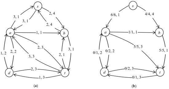
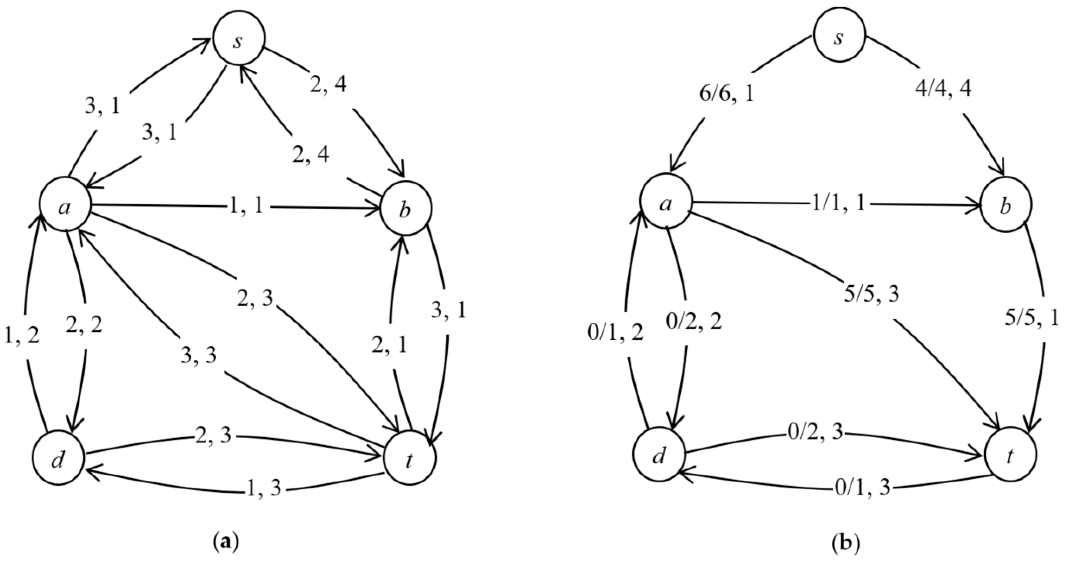
Consider a network shown in Figure 1a. The arc labels represent capacity, travel time. With the time horizon of $T=10$, the static flow corresponding to the temporally repeated maximum dynamic contraflow (maximum dynamic flow with arc reversals) is shown in Figure 1b. Each arc label represents flow/capacity and time. The value of the static flow is 10 and that of the dynamic flow is $10\times 10-\left(6\times 1+4\times 4+1\times 1+5\times 1+5\times 3\right)=57$. So the static flow in Figure 1b represents the static flow corresponding to the temporally repeated quickest flow with $Q=57$ and the quickest time 10.

In Figure 1b, we see that all the paths towards source $s$ are blocked because of the arc reversals. If one saves a path from specific node $d$ to $s$, the quickest time increases. In what follows, the length of directed path $P$ is $\tau \left(P\right)={\displaystyle \sum }_{\left(i, j\right)\in P}{\tau }_{ij}$.

Example 2.

Consider the network given in Figure 1a. Given $Q=57$, if we save path $d-a-s$, i.e., allow arc reversals in the arcs except those in the path $d-a-s$, then the quickest time increases to 12.57. The saved paths, their lengths and the corresponding quickest times are shown in

Table 1. Saved paths, their lengths and the corresponding quickest time of the dynamic contraflow with $Q=57$.

Saved Path (P)	Saved Length τ(P)	Quickest Time
P1: d − a − s	3	12.57
P2: d − t − a − s	7	12.57
P3: d − a − b − s	7	11.63
P4: d − t − b − s	8	11.25
P5: d − a − t − b − s	10	11.75
P6: d − t − a − b − s	11	16.20

.

In the above example, if we consider the quickest time only, the optimal path is $P_4:d-t-b-s$. However, if we also consider the length of the path, the decisions may be different, e.g., if the path length cannot exceed 7, the optimal path would be $P_3$. This motivates a bicriteria model with the objectives of minimizing the length of the saved path and minimizing the quickest time horizon of the dynamic contraflow. For the development of such a model, the following results are helpful.

Theorem 2.

If every cycle in $N$ is of positive length, the static flow corresponding to the quickest flow in the solution of (11)–(13) does not have a positive flow in a cycle.

Proof. 

Suppose that

$$T\left(x\right)=\frac{Q+{\sum }_{\left(i,j\right)\in A}{\tau }_{ij}{x}_{ij}}{v\left(x\right)}$$

for static flow $x$ in $N$. Let $x^{*}$ be a solution of (11)–(13) with $v\left(x^{*}\right)=v^{*}$, and assume that a flow decomposition of $x^{*}$ has a positive flow in cycles. Suppose that $C$ is the set of arcs that form a cycle with a flow value $\delta >0$. Define $x^1,x^2:A\to ℝ$ by

$$x_{ij}^1=\{\begin{array}{ll}{x}_{ij}^{*},\hfill & \left(i,j\right)\in A\setminus C\hfill \\ x_{ij}^{*}-\delta ,\hfill & \left(i,j\right)\in C\hfill \end{array}$$

and

$$x_{ij}^2=\{\begin{array}{ll}0,\hfill & \left(i,j\right)\in A\setminus C\hfill \\ \delta ,\hfill & \left(i,j\right)\in C\hfill \end{array}.$$

Then $x^1$ and $x^2$ are feasible static flows in $N$ and $x=x^1+x^2$ such that $v\left(x^{*}\right)=v\left(x^1\right)$ because a flow in a cycle does not contribute to the value of the static flow. So,

$$\begin{array}{cc}T\left(x^{*}\right)\hfill & =\frac{Q+{\sum }_{\left(i,j\right)\in A}{\tau }_{ij}{x}_{ij}^{*}}{v\left(x^{*}\right)}\hfill \\ & =\frac{Q+{\sum }_{\left(i,j\right)\in A}{\tau }_{ij}{x}_{ij}^1+{\sum }_{\left(i,j\right)\in A}{\tau }_{ij}{x}_{ij}^2}{v^{*}}\hfill \\ & =\frac{Q+{\sum }_{\left(i,j\right)\in A}{\tau }_{ij}{x}_{ij}^1+\delta {\sum }_{\left(i,j\right)\in A}{\tau }_{ij}}{v^{*}}\hfill \\ & >\frac{Q+{\sum }_{\left(i,j\right)\in A}{\tau }_{ij}{x}_{ij}^1}{v\left(x^1\right)}=D\left(x^1\right).\hfill \end{array}$$

This contradicts the optimality of $x^{*}$. □

If the transit time in each of the arcs of a network is positive, then every cycle in the network is of positive length and we have the following theorem.

Theorem 3.

If${\tau }_{ij}>0, \forall \left(i,j\right)\in A$, then a flow decomposition of an optimal solution$x^{*}$of the problem (11)–(13) does not contain a positive flow in a cycle.

The theorem leads to the following:

Theorem 4.

Given a network$N=\left(V,A,s, t, u,\tau \right)$with a supply$Q$at$s$, if (i)$\left(j,i\right)\in A$for each$\left(i, j\right)\in A$such that${\tau }_{ij}={\tau }_{ji}>0$, then a solution of the linear programming problem

$$\min \frac{Q+{\sum }_{\left(i, j\right)\in A}{\tau }_{ij}{x}_{ij}}{v}$$

(14)

subject to:

$${\displaystyle \sum }_{j\in V_i^{+}}{x}_{ij}-{\displaystyle \sum }_{j\in V_i^{-}}{x}_{ji}=\{\begin{array}{cc}\hfill v& \mathrm{for} i=s\hfill \\ \hfill -v& \mathrm{for} i=t\hfill \\ \hfill 0& \mathrm{for} i\in V\setminus \left\{s, t\right\}\hfill \end{array}$$

(15)

$$0\le x_{ij}\le u_{ij}+u_{ji}, \forall \left(i, j\right)\in A,$$

(16)

is also a solution of the quickest contraflow problem with$\left(i,j\right)$reversed if$x_{ji}>u_{ji}$.

Proof. 

Let $x$ be a solution of the problem (14)–(16). According to Algorithm 1, the quickest contraflow problem can be solved by solving the quickest flow problem in the auxiliary network so that $x_{ij}$ is bounded by $u_{ij}+u_{ji}$ for each $\left(i,j\right)\in A$. Further, Theorem 3, guarantees that there are no positive flows in the flow decomposition of $x$ so that Step 3 of the algorithm can be skipped and the result follows. □

Based on the above results, we formulate a bicriteria model as follows. Given a network $N=\left(V,A,s,t,u,\tau \right)$ with a supply $Q$ at $s$ and a specific node $d\in V$. Let

$${\psi }_1={\displaystyle \sum }_{\left(i,j\right)\in A}{\tau }_{ij}{y}_{ij}$$

(17)

$${\psi }_2=\frac{Q+{\sum }_{\left(i, j\right)\in A}{\tau }_{ij}{x}_{ij}}{v}$$

(18)

The problem is

$$\min \left({\psi }_1,{\psi }_2\right)$$

(19)

subject to

$${\displaystyle \sum }_{j\in V_i^{+}}{y}_{ij}-{\displaystyle \sum }_{j\in V_i^{-}}{y}_{ji}=\{\begin{array}{cc}\hfill -1& \hfill if i=s\\ \hfill 0& \hfill if i\in V\\ \hfill 1& \hfill if i=d\end{array}\setminus \left\{s, d\right\}$$

(20)

$$y_{ij}\le u_{ij}, \forall \left(i, j\right)\in A$$

(21)

$${\displaystyle \sum }_{j\in V_i^{+}}{x}_{ij}-{\displaystyle \sum }_{j\in V_i^{-}}{x}_{ji}=\{\begin{array}{cc}\hfill v& \hfill if i=s\\ \hfill 0& \hfill if i\in V\\ \hfill -v& \hfill if i=t\end{array}\setminus \left\{s, t\right\}$$

(22)

$$0\le x_{ij}\le \left(1-y_{ij}\right)u_{ij}+\left(1-y_{ji}\right)u_{ji}, \forall \left(i,j\right)\in A$$

(23)

$$y_{ij}\in \left\{0, 1\right\}$$

(24)

Constraints (20), (24) construct a $d$-$s$ path. Constraints (21) ensure that such a path does not contain a path zero-capacity path. Constraints (22) and (23) send a static flow of value $v$ from $s$ to $t$ allowing arc reversals in the network except the arcs in the path constructed by (20), (21), (24). The objective (19) minimizes the length of the path and the quickest time of the dynamic flow formed by the temporal repetition of the static flow $x$.

We use the idea given by Ehrgott [13] to get the weakly Pareto optimal (weakly efficient) solutions. This is done by minimizing ${\psi }_2$ and adding a constraint ${\psi }_1\le ϵ, ϵ\in ℝ$. Since ${\psi }_2$ is not linear, we put $1/v=\omega ,x_{ij}/v={\xi }_{ij}$ to make it linear. As a result, constraints (23) become non-linear. We put $\left(1-y_{ij}\right)\omega ={\zeta }_{ij}$ and use the idea given by Torres [14] to obtain the following mixed-integer linear program.

$$\min {\psi }_2=Q\omega +{\displaystyle \sum }_{\left(i, j\right)\in A}{\tau }_{ij}{\xi }_{ij}$$

(25)

Subject to

$${\displaystyle \sum }_{j\in V_i^{+}}{y}_{ij}-{\displaystyle \sum }_{j\in V_i^{-}}{y}_{ji}=\{\begin{array}{cc}\hfill -1& if i=s\hfill \\ \hfill 0& if i\in V\hfill \\ \hfill 1& if i=d\hfill \end{array}\setminus \left\{s, d\right\}$$

(26)

$$y_{ij}\le u_{ij}, \forall \left(i, j\right)\in A$$

(27)

$${\displaystyle \sum }_{j\in V_i^{+}}{\xi }_{ij}-{\displaystyle \sum }_{j\in V_i^{-}}{\xi }_{ji}=\{\begin{array}{cc}\hfill 1& if i=s\hfill \\ \hfill 0& if i\in V\hfill \\ \hfill -1& if i=t\hfill \end{array}\setminus \left\{s, t\right\}$$

(28)

$$0\le {\xi }_{ij}\le {\zeta }_{ij}{u}_{ij}+{\zeta }_{ji}{u}_{ji}, \forall \left(i,j\right)\in A$$

(29)

$$0\le {\zeta }_{ij}\le \omega ,\forall \left(i,j\right)\in A$$

(30)

$$\omega -y_{ij}\le {\zeta }_{ij}\le 1-y_{ij}, \forall \left(i, j\right)\in A$$

(31)

$${\displaystyle \sum }_{\left(i,j\right)\in A}{\tau }_{ij}{y}_{ij}\le ϵ$$

(32)

$$y_{ij}\in \left\{0, 1\right\}$$

(33)

As ${\psi }_1$ is the length of a path, when transit time ${\tau }_{ij}\in {\mathbb{Z}}_{>0}, \forall \left(i,j\right)\in A$, we construct Algorithm 2, which finds the set of non-dominated paths corresponding to all the non-dominated points of the feasible set in the objective space.

Algorithm 2. Non-dominated paths with the quickest contraflow.

Input$: N=\left(V, A, u, \tau , s, t\right) \mathrm{with} \mathrm{a} \mathrm{depot} \mathrm{node} d, \mathrm{and} \mathrm{supply} Q \mathrm{at} \mathrm{the} \mathrm{source} s \mathrm{with} u_{ij}\in {\mathbb{Z}}_{\ge 0}, {\tau }_{ij}\in {\mathbb{Z}}_{>0}\forall \left(i, j\right)\in A$

Output: A set of non-dominated saved paths with the quickest contraflow ${ϵ}_0=$ length of the shortest d–s path, $L=\varnothing , {\psi }_2^0=\infty$$, {ϵ}_1=1+\sum _{\left(i,j\right)\in A}{\tau }_{ij}$$, k=1$. $\mathrm{While} {ϵ}_k>{ϵ}_0$, $Z_k=$ solution of Problem (25)–(33)$\mathrm{for} ϵ={ϵ}_k-1$ $L=L{{\displaystyle \cup }}^{ }\left\{Z_k\right\}$ ${\psi }_1^k={\psi }_1\left(Z_k\right),{\psi }_2={\psi }_2\left(Z_k\right)$ $\mathrm{If} {\psi }_2^k={\psi }_2^{k-1}$$, L=L\setminus \left\{Z_k\right\}$ ${ϵ}_{k+1}={\psi }_1^k$$, k=k+1$ $\mathrm{For} \mathrm{each} Z\in L$, construct a path using y-values and quickest contraflow using x-values.

For each $ϵ\in ℝ$, a solution of (25)–(33) is a weakly-efficient solution of (19)–(24) according to [13]. If the transit time on arcs is allowed to take only integral values, $ϵ$ can also be taken as a positive integer ranging from the length of the shortest path to $\sum _{\left(i,j\right)\in A}{\tau }_{ij}$. Because of the Step 2d in Algorithm 2, we have the following result.

Theorem 5.

Algorithm 2 gives a set of non-dominated paths corresponding to all the non-dominated points of feasible set in the objective space of (19)–(24).

4. Conclusions

To optimize the flow during emergency evacuation, sometimes it is pertinent to save a path towards the hazardous area for the transportation of some facilities. We have developed a bicriteria model that minimizes the length of the saved path and the quickest time of evacuees allowing reversal of the direction of the evacuee flow in appropriate road segments. We present a solution algorithm based on $ϵ$-constraint approach of finding efficient solution of a multicriteria optimization problem.

References

- Dhamala, T.N.; Pyakurel, U.; Dempe, S. A critical survey on the network optimization algorithms for evacuation planning problems. Int. J. Oper. Res. 2018, 15, 101–133. [Google Scholar]
- Kim, S.; Shekhar, S.; Min, M. Contraflow transportation network reconfiguration for evacuation route planning. IEEE Trans. Knowl. Data Eng. 2008, 20, 1115–1129. [Google Scholar]
- Rebennack, S.; Arulselvan, A.; Elefteriadou, L.; Pardalos, P.M. Complexity analysis for maximum flow problems with arc reversals. J. Comb. Optim. 2018, 19, 200–216. [Google Scholar] [CrossRef]
- Pyakurel, U.; Dhamala, T.N. Continuous dynamic contraflow approach for evacuation planning. Ann. Oper. Res. 2017, 253, 573–598. [Google Scholar] [CrossRef]
- Hamacher, H.W.; Heller, S.; Rupp, B. Flow location (FlowLoc) problems: Dynamic network flow and location models for evacuation planning. Ann. Oper. Res. 2013, 207, 161–180. [Google Scholar] [CrossRef]
- Nath, H.N.; Pyakurel, U.; Dhamala, T.N.; Dempe, S. Dynamic network flow location models and algorithms for quickest evacuation planning. J. Ind. Manag. Optim. 2021, 17, 2925–2941. [Google Scholar] [CrossRef]
- Nath, H.N.; Dempe, S.; Dhamala, T.N. A bicriteria approach for saving a path maximizing dynamic contraflow. Asia-Pac. J. Oper. Res. 2021. [Google Scholar] [CrossRef]
- Ahuja, R.K.; Magnanti, T.L.; Orlin, J.B. Network Flows: Theory, Algorithms, and Applications; Prentice Hall: Upper Saddle River, NJ, USA, 1993. [Google Scholar]
- Ford, L.R.; Fulkerson, D.R. Constructing maximal dynamic flows from static flows. Oper. Res. 1958, 6, 419–433. [Google Scholar] [CrossRef]
- Skutella, M. An Introduction to Network Flows Over Time. In Research Trends in Combinatorial Optimization; Springer: Berlin, Germany, 2009; pp. 451–482. [Google Scholar]
- Lin, M.; Jaillet, P. On the quickest flow problem in dynamic networks: A parametric network flow min-cost flow approach. In Proceedings of the Twenty-Sixth Annual ACM-SIAM Symposium on Discrete Algorithms, San Diego, CA, USA, 4–6 January 2015; Society for Industrial and Applied Mathematics: San Diego, CA, USA, 2015; pp. 1343–1356. [Google Scholar]
- Pyakurel, U.; Nath, H.N.; Dhamala, T.N. Efficient contraflow algorithms for quickest evacuation planning. Sci. China Math. 2018, 61, 2079–2100. [Google Scholar] [CrossRef]
- Ehrgott, M. Multicriteria Optimization, 2nd ed.; Springer Science & Business Media: Berlin, Germany, 2005. [Google Scholar]
- Toress, F.E. Linearization of mixed integer products. Math. Program. 1990, 49, 427–428. [Google Scholar] [CrossRef]
Publisher’s Note: MDPI stays neutral with regard to jurisdictional claims in published maps and institutional affiliations. |
© 2022 by the authors. Licensee MDPI, Basel, Switzerland. This article is an open access article distributed under the terms and conditions of the Creative Commons Attribution (CC BY) license (https://creativecommons.org/licenses/by/4.0/).