Abstract
Accurate forecasts play a crucial role in various industries, where enhancing forecast accuracy has been a major focus of research. However, for volatile data and industrial applications, ensuring the reliability and interpretability of forecast results is equally important. This study shifts the focus from predicting future values to estimating forecast accuracy with confidence when no future validation data is present. To achieve this, we use time series characteristics calculated by statistical tests and estimate forecast accuracy metrics. For this, two methods are applied: Estimation by the euclidean distances between time series characteristic values, and second, estimation by clustering of time series characteristics. In-sample forecast accuracy serves as a benchmark method. A diverse, industrial data set is used to evaluate the methods. The results demonstrate that there is significant correlation between certain time series characteristics and estimation quality of forecast accuracy metrics. For all forecast accuracy metrics, the two proposed methods outperform the in-sample forecast estimation. These findings contribute to improving the reliability and interpretability of forecast evaluations, particularly in industrial applications with unstable data.
1. Introduction
Accurate forecasting plays a crucial role across various industries, influencing decision-making processes f.e. in supply chain management, finance, and operations. Traditionally, forecast accuracy is assessed by comparing predicted values against actual future observations. Various metrics have been established in forecasting literature to evaluate accuracy when future observations are available. A meaningful benchmark are the Makridakis Competitions (M-Competitions)—Large-scale competitions comparing forecasting models across diverse data sets. While these provide meaningful assessments of forecasting accuracy, they depend on the availability of future forecasted values for evaluation, making them unsuitable for scenarios where accuracy estimation must be conducted without direct validation against realized values [1]. Given these challenges, other than only calculating metrics with future test data, an alternative approach is required for evaluating forecast reliability when future observations are unavailable.
Some techniques have been developed to estimate accuracy without relying on future observations. Despite their advantages, these methods have notable limitations. Meta-learning lacks in explainability for the user, and depends on representative past data, making it unreliable when historical patterns fail to capture new trends [2]. Studies employing meta-learning approaches have evaluated accuracy through metrics such as Mean Absolute Error (MAE) and Root Mean Squared Error (RMSE) to determine how well learned patterns generalize across different time series [3]. Since these metrics are scale-dependent and do not take the scale of past values into consideration, further studies with relative, scale-independent metrics need conduction. On the other hand, in-sample cross-validation for uncertainty estimation is prone to overfitting, particularly for large and diverse data sets [4].
Additionally, uncertainty quantification techniques such as conformal prediction and Bayesian modeling focus on confidence intervals rather than forecast accuracy estimation itself [5,6,7]. These techniques are more effective at quantifying forecast dispersion rather than directly measuring accuracy.
Building on these efforts, this study aims at testing explainable and effective methodologies for estimating forecast accuracy metrics when future observations are unavailable. Through the evaluation of Euclidean distance-based similarity measures, clustering-based estimation techniques, and in-sample accuracy benchmarks, the goal is to establish a framework for improving forecast reliability in industrial applications.
2. Materials and Methods
For this study, three methods for the estimation of forecast accuracy metrics are tested on a diverse, industrial data set. In this chapter, details of the data set, the selected forecast accuracy metrics, and the estimation methods are explained.
2.1. Data Preparation
For the experiments, a real industrial sales data set was used that includes a number of n = 13,000 time series for the years 2016 to 2022. The time series exhibit a monthly frequency (freq = 12), have 70 time steps (l = 70) and are characterised by high diversity, as well as a lot of time series with a high degree of zero values.
For generating results of high statistical significance, time series cross validation was performed. The data set was split in training, validation and test data, and seperated in 5 rolling windows with sizes of 48 (4 years) each.
2.2. Forecast Accuracy Metrics
For adaptivity to the data set and high interpretability, relative and scale-independent forecast accuracy metrics were used for the estimation. The forecasts had a horizon of six months (h = 6) and were performed using AUTO-ARIMA (pmdarima), Holt-Winters (statsmodels), and Naive2 (self-implemented). The following forecast accuracy metrics were calculated for all data sets and splits:
- Relative percentage error (positive and negative);
- Relative quantity error (positive and negative);
- Relative residual bias (positive and negative).
Relative errors were considered due to the high uncertainty of the used time series data which requires consideration of the past values’ scale. For the purpose of interpretation, positive and negative errors were calculated and outlined separately. The relative percentage error is used for easy interpretation. The relative quantity error takes aggregated time series values into consideration, and therefore assesses quantity deviations. Lastly, the relative residual bias checks for biases in the residuals (actual minus forecasted values). Positive metric values indicate that the forecast was higher than the actual values (over-forecast), and negative metric values indicate an under-forecast.
2.3. Uncertainty Estimation Methods
In this study, the estimation of the forecast accuracy metrics includes a single point estimation, and a 95% interval estimation, for each metric. For the estimation of the listed forecast accuracy metrics, three methods were considered:
- 1.
- In-Sample Residuals;
- 2.
- Euclidean Distances of Time Series Characteristics, and
- 3.
- Clustering of Time Series Characteristics.
The first method (1) is using the forecast accuracy metrics calculated for the in-sample forecast. For this, a rolling window is used on the in-sample residuals and the forecast accuracy metrics calculated for each window. The result is a quantity of forecast accuracy metric values. The second (2) and third (3) methods use characteristics of the time series data set that are derived by using selected statistical tests. In this study, two time series characteristics are combined each for the estimation of the forecast accuracy metrics in all possible combinations. For the second approach (2), euclidean distances are used for finding the nearest training time series characteristic combination. Their forecast accuracy metric values are used for the estimation. For the third method (3), euclidean-distance based clustering is performed on the time series characteristic combinations. KMeans, Hierarchical and Density Clustering are used with cluster center sizes optimized by the elbow method with the within-sum-of-squares (WSS). The forecast accuracy metric values of training time series of the nearest cluster are used for the estimation. For performing the second (2) and third method (3), the time series characteristics are calculated by six selected statistical tests:
- Augmented Dickey–Fuller (ADF) test: Assesses the null hypothesis that a unit root is present in a time series, values < 0.05 indicating stationarity [8].
- Complexity Entropy: Describes the irregularity, complexity, and unpredictability of a time series, where the value zero means it is perfectly predictable [9].
- Hurst Exponent: Characterises the long-term memory of the time series and therefore its autocorrelation, with values of 0.5 indicating randomity, values < 0.5 describing anti-persistence and values > 0.5 persistence [10].
- Kwiatkowski-Phillips-Schmidt-Shin (KPSS) test: Tests for stationarity with values < 0.05 indicating stationarity [11].
- Ljung-Box test: Detects autocorrelation in a time series with values < 0.05 indicating significant autocorrelation [12].
- Wald–Wolfowitz runs (Runs) test: Determines the randomness of a time series with values < 0.05 detecting patterns in the time series and therefore non-randomity [13].
2.4. Procedure
The estimation of the forecast accuracy metrics is performed on the training and validation data. For each estimation method, median and 95% confidence intervals are calculated as outputs of the estimation, and serve as point and interval estimation. The evaluation of the estimation is performed on the test data. Point estimations are validated by the relative percentage error to the actual forecast accuracy metrics. Interval estimations are evaluated by the relative widths of the interval, and the mean scaled interval score. For transforming the percentage error, interval width and mean interval score into relative measures, the scale of the training data’s forecast accuracy metrics is used, after removing extreme outliers.
3. Results
First, the relationship of time series characteristics and the estimation quality of the forecast accuracy metrics is analyzed. Second, the focus lies on the correlation of forecast accuracy metric values and their ability to be estimated sufficiently. For both, interval estimations are considered. Lastly, the three estimation methods are evaluated and compared by their point and interval estimation.
3.1. Time Series Characteristics and Estimation Quality
Figure 1 shows the values of the six statistical tests (x-axis), the relative widths (y-axis) and mean scaled interval score (short MSIS, colorbar) of the estimated intervals of the forecast accuracy metrics, using smoothed contour plots. Since the focus here lies on describing general relationships, outliers were removed for providing sufficient scaling of the plots.
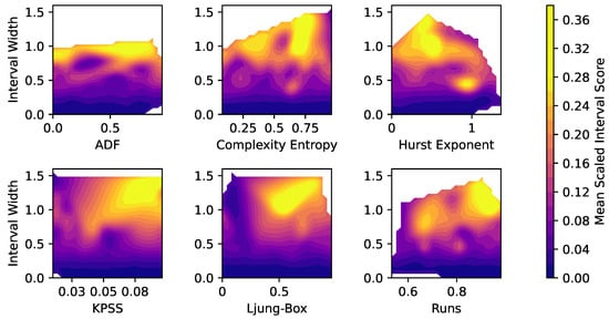
Figure 1.
Relationship of statistical test results, relative widths and Mean Scaled Interval Score (MSIS) of the interval estimation of the forecast accuracy metrics. (Outliers removed).
The figure clearly shows that higher relative interval widths (y-axis) correlate with higher MSIS values (yellow coloring). This seems intuitive because time series with wider uncertainty intervals usually inhibit a higher degree of uncertainty.
For the ADF test (upper left), there is a slight trend towards a positive correlation with estimation uncertainty visible. For the KPSS test (bottom left), this correlation appears strongly. Since both ADF and KPSS detect stationarity in a time series with low values indicating stationarity, non-stationarity seems to correlate with higher estimation uncertainty. Regarding the Complexity Entropy (upper center), there is a positive correlation of complexity and estimation error visible. This seems reasonable, as higher time series complexity inhibits higher uncertainty in the forecast accuracy estimation. The Hurst Exponent (upper right) shows high interval widths and high MSIS values around values of H = 0.5 Due to the fact that a Hurst Exponent around 0.5 describes randomity of a time series, and lower or higher values anti-persistence and persistence of a time series, this seems reasonable. For the Ljung-Box test (bottom center), higher test statistics (values from 0.3 to 0.8) show much higher MSIS values. This makes sense, since low Ljung-Box values indicate the existence of significant autocorrelation in the time series, and higher values therefore low or no autocorrelation. Lastly, for the Runs test (bottom right), higher runs values correlate slightly with higher interval widths and MSIS values. Since Runs detects randomity in time series, with higher Runs values indicating randomity, these results seem intuitive.
3.2. Forecast Accuracy and Estimation Quality
Next, the relationship between actual forecast accuracy metric values and the quality of their interval estimation will be analyzed. Figure 2 displays the six forecast accuracy metrics (x-axis), and the relative width (y-axis) and the Mean Scaled Interval Score (MSIS, colorbar) of the uncertainty estimation interval. As the focus lies on detecting basic relationships, outliers are removed from the plot to provide proper scaling.
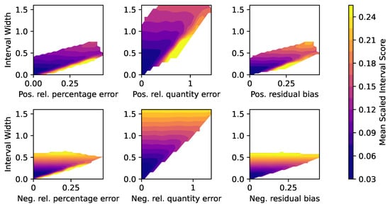
Figure 2.
Relationship of forecast accuracy metrics, relative widths and Mean Scaled Interval Score (MSIS) of the interval estimation of the forecast accuracy metrics. (Outliers removed).
It is visible that there is a general but not consistent trend in the plots of a positive correlation between interval widths and MSIS values. It clearly appears that the quantity errors, both positive (upper center) and negative (lower center), exhibit the highest relative interval widths. Since the quantity error considers aggregated values from a time series, errors might be aggregated as well and therefore wider intervals result. For all forecast accuracy metrics, low interval widths and MSIS values (dark blue color) appear at low metric values. This relationship appears reasonable as low forecast accuracy errors correlate with a lower uncertainty in their estimation.
3.3. Evaluation of the Uncertainty Estimation
Lastly, it is analyzed how the three estimation methods perform based on their point and interval estimation. Figure 3 displays the relative percentage error (y-axis) of the point estimation from the actual forecast accuracy metrics for each of the six metrics for the in-sample estimation (ins.), the euclidean distances of the time series characteristics (euc.), and the clustering of the time series characteristics (clu., x-axis). Outliers were removed again to ensure sufficient scaling.
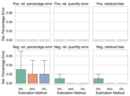
Figure 3.
Point Estimation Evaluation with the relative percentage error of the estimation methods in-sample (ins.), euclidean distances of time series characteristics (euc.), and clustering of time series characteristics (clu.), for the six forecast accuracy metrics. (Outliers removed).
For the positive metrics (upper row), the relative percentage error is lower than <0.0001. This fact speaks for a high quality of the point estimation of the positive metrics (except for outliers). The lower estimation performance for negative metric estimation might stem from the fact that the data set includes time series with a lot of zero values, which makes the forecasting models prone to under-forecasting. For the negative forecast accuracy metrics (bottom row), the in-sample estimations exhibit higher errors in the 0.75% percentile, and higher variance than for the other estimation methods.
Lastly, for evaluation of the interval estimation of the forecast accuracy metrics, Figure 4 displays the Mean Scaled Interval Score (MSIS, y-axis) for the estimation methods (x-axis). Note that positive (upper row) and negative (bottom row) metrics each have their own scale to ensure proper comparison.
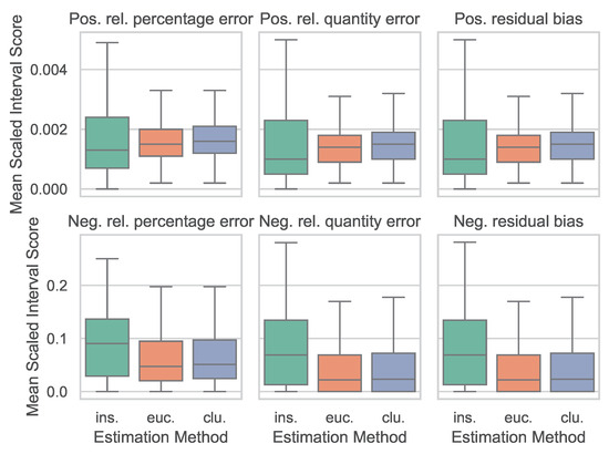
Figure 4.
Interval Estimation Evaluation with the Mean Scaled Interval Score (MSIS) of the estimation methods in-sample (ins.), euclidean distances of time series characteristics (euc.), and clustering of time series characteristics (clu.), for the six forecast accuracy metrics. (Outliers removed).
In this plot, positive forecast accuracy metric estimations are again of much higher quality with medians of MSIS = 0.2% than for the negative metrics that shows medians around MSIS = 10% The in-sample estimation has again higher estimation errors and higher variance of the MSIS than the other two methods.
3.4. Conclusions
In this study, three methods were evaluated and compared for the point and interval estimation of forecast accuracy metrics without presence of future validation data. Two methods used time series characteristics, derived by statistical tests, for the estimation. These methods include euclidean distances of the time series characteristics, and clustering of the time series characteristics. Plus, estimations with forecast accuracy metrics of the in-sample forecasts were used as a benchmark. The estimations include a point and an interval estimation.
The results showed clear, nearly linear relationships of certain time series characteristics and the quality of the forecast accuracy estimation. A low degree of significant autocorrelation (tested by Ljung-Box) correlated with higher estimation interval widths and interval estimation errors. Non-stationarity of time series (tested by ADF and KPSS) corresponded with lower estimation quality as well. A high degree of randomity of time series (tested by Hurst Exponent and Runs) exhibited wider estimation intervals and lower interval estimation quality. Lastly, complex time series (tested by Complexity Entropy) correlated with higher interval widths and interval estimation errors.
Forecast accuracy metric values and their estimation quality also showed clear trends. The relative quantity errors, both positive and negative, showed by far the highest relative interval widths and lowest estimation quality in comparison to the other metrics relative percentage error and relative residual bias. As quantity errors take aggregated values into considerations, errors might aggregate as well. For all forecast accuracy metrics, lower metric values correlated with lower interval widths and higher estimation quality.
The comparison of the estimation methods (euclidean distances, clustering, in-sample) shows that all three methods are capable of performing the point estimation with very low relative percentage errors near 0%. For both point and interval estimations, the in-sample method shows the lowest estimation quality compared to the other methods. Since the in-sample method is prone to overfitting, as it uses only past values of a time series instead of learning from a data set as the other methods do, this finding seems reasonable. Future research could explore improvement of the estimation methods by adding advanced machine learning techniques, such as neural networks or meta-learning, even though interpretability might be reduced. Additionally, the study could be performed on different data sets, including financial or medical data, to draw more general conclusions. Lastly, investigating the adaptability of the estimation methods to more forecasting methods or different forecasting horizons might be a valuable next step.
Author Contributions
Conceptualization, A.T.; methodology, A.T.; software, A.T. and A.P.; validation, A.T.; formal analysis, A.T.; investigation, A.P.; resources, A.T.; data curation, A.T. and A.P.; writing—original draft preparation, A.T. and A.P.; writing—review and editing, A.T. and A.P.; visualization, A.T.; supervision, A.T.; project administration, A.T.; funding acquisition, A.T. All authors have read and agreed to the published version of the manuscript.
Funding
This research was funded by the German Research Foundation (Deutsche Forschungsgemeinschaft, DFG) for Research Training Group 2193.
Institutional Review Board Statement
Not applicable.
Informed Consent Statement
Not applicable.
Data Availability Statement
The data presented in this study are available upon request from the corresponding author.
Conflicts of Interest
The authors declare no conflicts of interest.
Abbreviations
The following abbreviations are used in this manuscript:
| ARIMA | Autoregressive Integrated Moving Average |
| MSIS | Mean Scaled Interval Score |
References
- Voyant, C.; Notton, G.; Paoli, C.; Nivet, M.L. Benchmarks for Solar Radiation Time Series Forecasting. arXiv 2022, arXiv:2203.14959. [Google Scholar] [CrossRef]
- Varma, S.; Simon, R. Bias in error estimation when using cross-validation for model selection. BMC Bioinform. 2006, 7, 91. [Google Scholar] [CrossRef] [PubMed]
- Bergmeir, C.; Benítez, J.M. On the use of cross-validation for time series predictor evaluation. Inf. Sci. 2012, 191, 192–213. [Google Scholar] [CrossRef]
- Politis, D.N.; Romano, J.P. The stationary bootstrap. J. Am. Stat. Assoc. 1994, 89, 1303–1313. [Google Scholar] [CrossRef]
- Angelopoulos, A.N.; Bates, S. A Gentle Introduction to Conformal Prediction and Distribution-Free Uncertainty Quantification. arXiv 2021, arXiv:2107.07511. [Google Scholar]
- Vovk, V.; Gammerman, A.; Shafer, G. Algorithmic Learning in a Random World; Springer Science & Business Media: Berlin/Heidelberg, Germany, 2005. [Google Scholar]
- Gneiting, T.; Katzfuss, M. Probabilistic Forecasting. Annu. Rev. Stat. Its Appl. 2014, 1, 125–151. [Google Scholar] [CrossRef]
- Dickey, D.A.; Fuller, W.A. Distribution of the estimators for autoregressive time series with a unit root. J. Am. Stat. Assoc. 1979, 74, 427–431. [Google Scholar] [PubMed]
- Bandt, C.; Pompe, B. Permutation entropy: A natural complexity measure for time series. Phys. Rev. Lett. 2002, 88, 174102. [Google Scholar] [CrossRef] [PubMed]
- Hurst, H.E. Long-term storage capacity of reservoirs. Trans. Amer. Soc. Civil Eng. 1951, 116, 770–799. [Google Scholar] [CrossRef]
- Kwiatkowski, D.; Phillips, P.C.; Schmidt, P.; Shin, Y. Testing the null hypothesis of stationarity against the alternative of a unit root: How sure are we that economic time series have a unit root? J. Econom. 1992, 54, 159–178. [Google Scholar] [CrossRef]
- Ljung, G.M.; Box, G.E. On a measure of lack of fit in time series models. Biometrika 1978, 65, 297–303. [Google Scholar] [CrossRef]
- Wald, A.; Wolfowitz, J. On a test whether two samples are from the same population. Ann. Math. Stat. 1940, 11, 147–162. [Google Scholar] [CrossRef]
Disclaimer/Publisher’s Note: The statements, opinions and data contained in all publications are solely those of the individual author(s) and contributor(s) and not of MDPI and/or the editor(s). MDPI and/or the editor(s) disclaim responsibility for any injury to people or property resulting from any ideas, methods, instructions or products referred to in the content. |
© 2025 by the authors. Licensee MDPI, Basel, Switzerland. This article is an open access article distributed under the terms and conditions of the Creative Commons Attribution (CC BY) license (https://creativecommons.org/licenses/by/4.0/).