Article

Tree-Related Microhabitats and Multi-Taxon Biodiversity Quantification Exploiting ALS Data

1
Dipartimento di Bioscienze e Territorio, Università degli Studi del Molise, C. da Fonte Lappone, 86090 Pesche, Italy
2
NBFC, National Biodiversity Future Center, 90133 Palermo, Italy
3
geoLAB—Laboratorio di Geomatica Forestale, Dipartimento di Scienze e Tecnologie Agrarie, Alimentari, Ambientali e Forestali, Università degli Studi di Firenze, Via San Bonaventura 13, 50145 Firenze, Italy
4
CREA Research Centre for Forestry and Wood, Viale Santa Margherita, 52100 Pratovecchio, Italy
5
Forest Modelling Laboratory, Institute for Agriculture and Forestry Systems in Mediterranean, National Research Council of Italy (CNR-ISAFOM), 06128 Perugia, Italy
6
Fondazione per il Futuro delle Città, 50145 Firenze, Italy
7
Independent Researcher, 51035 Lamporecchio, Italy
*
Authors to whom correspondence should be addressed.
These authors contributed equally to this work.
Forests 2024, 15(4), 660; https://doi.org/10.3390/f15040660
Submission received: 13 March 2024 / Revised: 2 April 2024 / Accepted: 3 April 2024 / Published: 5 April 2024
(This article belongs to the Topic Mediterranean Biodiversity)

Abstract

:
The quantification of tree-related microhabitats (TreMs) and multi-taxon biodiversity is pivotal to the implementation of forest conservation policies, which are crucial under the current climate change scenarios. We assessed the capacity of Airborne Laser Scanning (ALS) data to quantify biodiversity indices related to both forest beetle and bird communities and TreMs, calculating the species richness and types of saproxylic and epixylic TreMs using the Shannon index. As biodiversity predictors, 240 ALS-derived metrics were calculated: 214 were point-cloud based, 14 were pixel-level from the canopy height model, and 12 were RGB spectral statistics. We used the random forests algorithm to predict species richness and the Shannon diversity index, using the field plot measures as dependent variables and the ALS-derived metrics as predictors for each taxon and TreMs type. The final models were used to produce wall-to-wall maps of biodiversity indices. The Shannon index produced the best performance for each group considered, with a mean difference of −6.7%. Likewise, the highest R2 was for the Shannon index (0.17, against 0.14 for richness). Our results confirm the importance of ALS data in assessing forest biodiversity indicators that are relevant for monitoring forest habitats. The proposed method supports the quantification and monitoring of the measures needed to implement better forest stands and multi-taxon biodiversity conservation.

1. Introduction

Forest ecosystems host 80% of terrestrial biodiversity. Therefore, the management and conservation of forest biodiversity are of primary importance [1]. To counteract the decline in biodiversity, long-term monitoring programs with a multi-taxonomic approach are needed [2,3].
In recent years, many studies have focused on the ecological relationships between forests’ structural variables and forest biodiversity indicators (e.g., tree-related microhabitats) and wildlife (e.g., beetles and birds) to identify models of biodiversity and priority areas for both management and conservation [4]. Thus, the structural complexity of forest habitats can help in predicting the compositional structure of animal communities [5].
The multi-taxon approach is frequently applied in forest stands to correlate specific forest characteristics useful for management and conservation practices [2]. Insects—including saproxylic (i.e., related to deadwood) and non-saproxylic beetles—and birds depend on forest composition and structure [6,7,8]. Ecological relationships between biodiversity indicators and forests’ structural attributes have been extensively analyzed [9,10,11]. The links between animal species and forest ecosystems can be examined by grouping species into ecological assemblages based on habitat characteristics and species ecology [12]—for example, trophic category, ecological characteristics, level of specialization (e.g., [13,14,15]). The assumption behind using ecological groups rather than individual species is related to consistent differences in response to changes in forest variables. Indeed, species sharing the same functional traits share similar ecological characteristics [16,17]. For example, forest bird assemblages broadly reflect similarities in forest structure, distribution, and the abundance of foraging resources [18]. This approach can highlight differential responses in species assemblages and help us to understand ecological relationships that can support targeted conservation strategies. Furthermore, if species of saproxylic beetles and birds show a strong dependence on the forest structure, they can be considered forest specialists [19,20], and as often happens can be promoted as indicators of forest biodiversity [21].
Forests’ structure components, such as tree height and diameter, canopy cover, the presence of deadwood, and tree-related microhabitat abundance, are assumed to be relevant for specific categories of organisms [5,21]. These ecological components strongly influence beetles and birds. Indeed, the vertical and horizontal structure of the forest influences the composition, abundance, density, and stability of animal communities [22,23].
Furthermore, animal communities thrive in structurally diverse forest habitats, such as old-growth, near-natural, or unmanaged forests [24,25]. Recently, many ecologically demanding species of beetle have experienced a steep decline [8], and despite the generally positive trend for forest birds [16], some forests still have a vulnerable conservation status [23]. This phenomenon is particularly evident for species living in structurally heterogeneous forests with large amounts of deadwood, where levels of specialization are particularly intense [24].
Remote sensing (RS), and specifically Airborne Laser Scanning (ALS or airborne Light Detection And Ranging—LiDAR) technology, has been widely used to quantify the heterogeneity and complexity of natural habitats in patterns of distribution or diversity of species or groups [25]. ALS enables the effective quantification of the vertical canopy structure over large areas. For example, ALS data provide information on canopy stratification or vertical structural heterogeneity, which is a key proxy variable for habitat structural features for insect and bird groups [26,27]. Furthermore, ALS predictors of vertical structure may help to explain the differentiation of ecological niches for closely related species [28]. RS for mapping small organisms, such as deadwood-dependent insects, presents significant challenges due to the secretive nature of many species and the constraints imposed by the resolution of the available data [29].
Although extensive efforts have been directed towards the detection and monitoring of forest pests [30] and of the associated forest disturbances, the use of ALS data to study the ecology and conservation of forest organisms remains only partially explored [31]. Similarly, studies exploiting RS data are still relatively rare [32,33]. The main advantage of approaches based on ALS data is their capacity to provide high-resolution topography and forest structures at large spatial scales within statistically correct data (e.g., [34,35,36]). Therefore, ALS data can be exploited to derive forest structure and variability information from which indicators of biodiversity can be extrapolated [31,37].
The aim of our study was (i) to assess the richness of specific microhabitats and the diversity of saproxylic and non-saproxylic beetle and bird communities, and (ii) to analyze the relationships between ALS-derived predictors and microhabitats and biodiversity measured in the field.

2. Materials and Methods
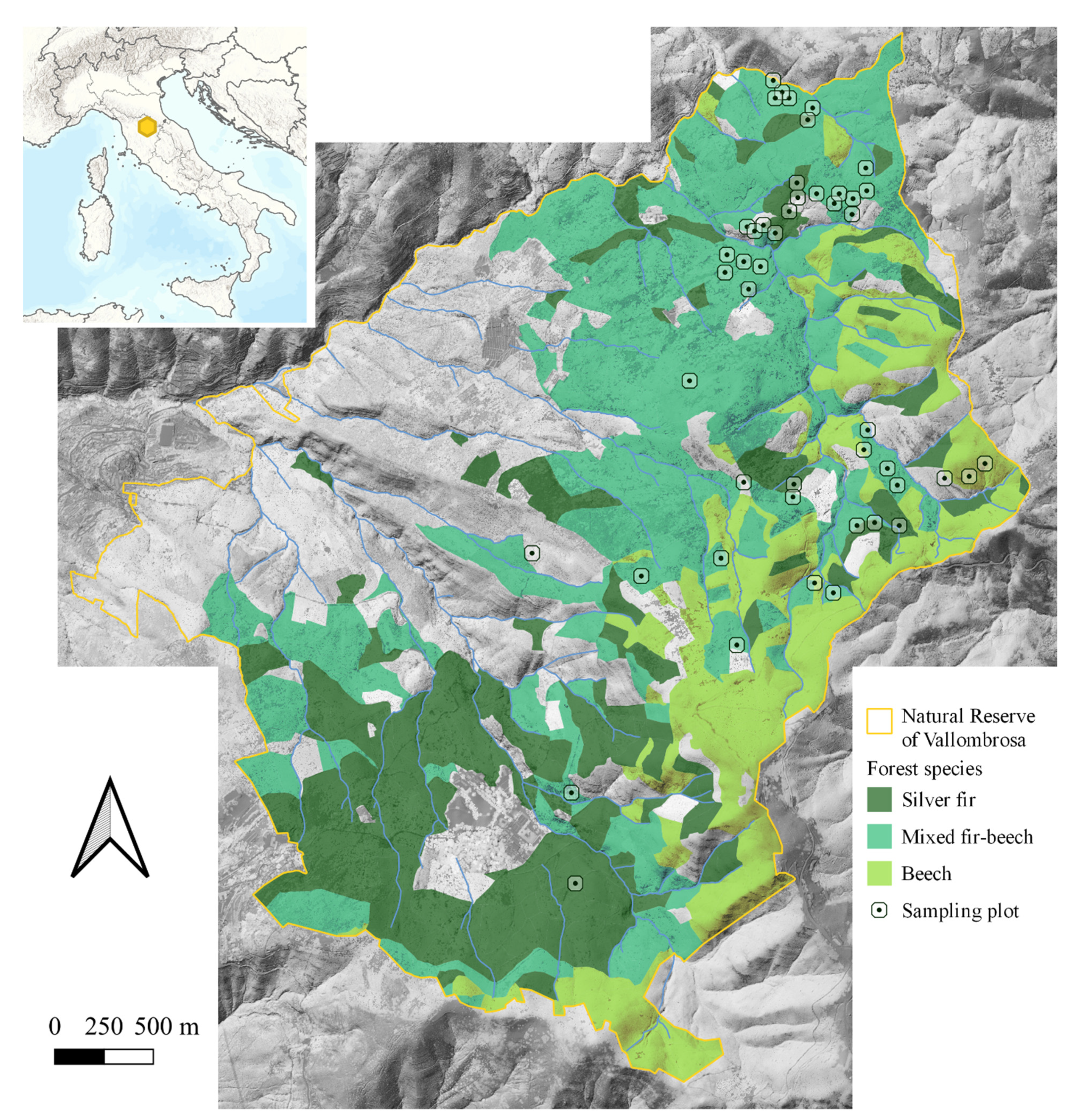
2.1. Study Area

We conducted our study in pure and mixed Fagus sylvatica and Abies alba stands within the Nature Reserve of Vallombrosa (43.745 E, 11.562 N), located in the Tuscany region, on the north-west side of the Pratomagno Massif (Italy) (Figure 1). The Reserve is part of the Natura 2000 Network, included within the Special Area of Conservation (SAC) “Vallombrosa e Bosco di S. Antonio” (code IT5140012), as defined by the EU Habitats Directive (92/43/EEC).
The Nature Reserve of Vallombrosa covers 1273 ha, with the altitude varying between 470 and 1447 m a.s.l. Pure even-aged stands of silver fir (Abies alba Mill.) are the primary forest type in the Reserve (664 ha), followed by pure beech (Fagus sylvatica L.) stands (187 ha), which mainly originated from the coppice conversion to high forest. Silver fir has been cultivated in pure stands in the Vallombrosa Forest for many centuries, but in recent decades, social, economic, and environmental changes have significantly changed forest management [38]. The last regulation plan, issued in 1970, has not been applied, and thus the forest structure and composition are slowly evolving, especially in the fir stands, where broadleaves are gradually coming in. A new Forest Management Plan was drawn out for the period 2006–2025 [38], based on the silvosystemic approach [39,40]; this plan favors the natural diversification of the forest towards mixed and structurally complex stands. In recent years, major windstorm events have sped up these changes [38].
Figure 1. Nature Reserve of Vallombrosa: silver fir, beech, and mixed fir–beech stand locations and sampling plot distribution [41].
Forests 15 00660 g001
Other forest types included in the Reserve are Pinus nigra J.F. Arnold, Pseudotsuga menziesii (Mirb.) Franco, introduced for experimental purposes, and deciduous mixed forests of Castanea sativa Mill., Quercus cerris L., Q. pubescens Willd., Ostrya carpinifolia Scop., and Fraxinus ornus L., but these forest types were not considered in our study.
Detailed information on the Reserve was derived from forest management plans developed over the years. Specifically, for each forest stand (i.e., management unit), information on elevation, aspect, slope, site quality, forest type, stand age, and year of the last cut was derived from the forest management plan 2006–2025 [39].

2.2. Reference Data for Biodiversity Indices

The reference dataset consisted of 47 circular sampling plots with a 13 m radius located within the Reserve in F. sylvatica and A. alba pure and mixed stands (Figure 1). The plots were located at elevations between 900 and 1250 m a.s.l., with a minimum slope of 9% and a maximum of 48%. The stand age varied from 50 to 180 years old. Twenty-seven plots fell in mixed stands, while the remaining fell equally in pure stands. Field surveys were conducted in 2020 to collect the data needed to quantify forest biodiversity indices related to microhabitats, beetles, and birds. More details on these surveys are provided in the following sections.

2.2.1. Beetle Communities

In the 47 sampling plots, saproxylic and non-saproxylic adult beetles were captured using window flight traps [10]. At the center of each sampling plot, one window flight trap was positioned at a height of two meters above ground on a tree branch to catch flying beetles and was checked monthly (from May to October) for a total of four surveys. All the monitoring systems were then removed during the winter.
Systematics and the nomenclature of beetle species were performed by following Bouchard et al. [42] and Audisio et al. [43]. For further analysis, species strictly considered saproxylic (sensu Carpaneto et al., [21]) were reported, with their IUCN Red list risk category at the Italian level and their trophic categories (see [21]). Saproxylic beetles were analyzed separately and also aggregated with non-saproxylic beetles.

2.2.2. Birds

The bird census was carried out using a standardized area count method [44]; 47 hexagon-shaped plots were identified, each spanning 1.25 ha and including one 13 m-radius plot. All the plots were surveyed twice (in March and April, 5′ each time). The locations of all observed birds were recorded on a detailed map (scale 1:1500 with satellite images + Technical Regional Maps) in order to consider only the birds inside each plot accurately and exclude those outside of it. All birds heard or seen within the plots were recorded. Systematics and nomenclature of bird species followed [45].

2.2.3. Tree-Related Microhabitats

Tree-related microhabitats (TreMs) were censused in each 13 m-radius sampling plot, carefully observing both deadwood (standing dead trees, dead downed trees, snags and stumps, e.g., saproxylic holes, presence of tunnels or fungi) and living trees (e.g., broken crowns, presence of cavities on the trunks). The identification was based on the reference list developed by [46], which defines 64 different microhabitat types, divided into two main categories: saproxylic microhabitats (whose origin is due to impacts of a biotic or abiotic nature that expose sub-cortical portions of the plant), and epixylic microhabitats (due to elements of external origin physically connected to the tree, such as fungal fruiting bodies) (Supplementary Material Table S1).
The types and abundance (frequency of all types) of TreMs were counted with binoculars for living trees or standing dead trees and through the direct observation of deadwood components on the ground. The microhabitat categories (saproxylic and epixylic) were analyzed both separately and aggregately.

2.3. Biodiversity Indices

Two biodiversity indices were calculated considering fauna species and TreMs types. The first is richness, defined as the number of species or TreMs types in each plot. Then, considering both richness and abundance, the Shannon Index was calculated:
H = i = 1 S p i l o g p i
where S is the total number of species or microhabitat types, and pi is the abundance of ith species or TreMs types.

2.4. Predictor Variables for Modeling Biodiversity Indices

2.4.1. Airborne Laser Scanning Variables

The ALS data were derived from a survey carried out in May 2015 with a LiDAR RIEGL LMS-Q680i (Horn, Austria) sensor and a DIGICAM H39 RGB and CIR optical instrument mounted in Eurocopter AS350 B3. The planned flight height was 1100 m above terrain level with a speed of 70 knots and an overlap between the strip of 30%. The sensor acquired full-waveform LiDAR data with a point density of 10 points m−2. ALS data were georeferenced in the WGS84 UTM32N coordinate system by correcting the flight trajectories with the Global Navigation Satellite System and the Inertial Measurement Unit collected data based on two base stations of the Italtopos network [47]. LAStools software (version 240220) (Gilching, Germany) was used for common ALS data preprocessing procedures (e.g., outliers and noise cleaning, classification of ground/non-ground points, and computation of height) [48].
A total of 240 ALS metrics were computed either directly from the point cloud (n = 214) or at the pixel level, using a rasterized canopy height model (CHM) (n = 14) with a spatial resolution of 1 m, together with RGB spectral statistics (n = 12) derived from aerial images. The point cloud metrics included metrics related to the z and intensity values and the combination of the two. Because of the two-dimensionality of the raster data, the CHM-derived variables describe the horizontal characteristics of the forest canopy [49]. Specifically, the CHM textural variables (grey-level co-occurrence matrices—GLMC) were computed using the R package GLCM with a 1 m × 1 m window size in all directions. The algorithm examines image textures and calculates the frequency with which pairs of pixels with specific values in a given spatial relationship occur in an image. For each field plot, we calculated mean, variance, homogeneity, contrast, dissimilarity, entropy, and second-moment textural variables, then used them to compute the plot’s level average and the standard deviation.
We calculated 214-point cloud metrics developed for each plot to represent the entire vertical forest structure (Supplementary Material Table S2). These included essential statistical variables [50], height, and density metrics typically used in forest inventory analysis [51]. The essential statistical variables are the total number of points (tot), the sum of the heights (sum), mean height (avg), height standard deviation (sd), skewness of height (sk), kurtosis of height (kur), and average square height (qav) [47,50]. The height metrics are height percentiles (p10, …, p100) calculated between the 100th percentile and a minimum threshold of 1.3 m. The density metrics were calculated for equally spaced vertical layers, defined as tenths of the distance between the 95th percentile and the lowest canopy height (i.e., 1.3 m). The densities were computed as the proportion of points above the 1st, …, 9th (d0, …, d9) spaced vertical layers to the total number of points.

2.4.2. Auxiliary Variables

We used the Digital Terrain Model (DTM) derived from the ALS data as an auxiliary variable to calculate the slope and the aspect of the field plots. In addition, we used the wall-to-wall growing stock volume (GSV) map produced by [52] for the year 2019 to extract the GSV for each plot. This map was obtained using a spatial approach to estimate forest inventory variables for the years not covered by a national forest inventory, considering the GSV current increment and the forest disturbances occurring during the time elapsed between the two updating cycles. The four auxiliary variables (DTM, slope, aspect, and GSV), which were in grid format, were resampled with the nearest neighbor algorithm at 23 m × 23 m spatial resolution, whose size mimicked the area of the plots measured in the field.

2.5. Random Forests Models

Random forests (RF) is an ensemble learning model based on decision trees that grows multiple trees using the CART (classification and regression tree) methodology [53,54]. Each tree is built using different training subsets generated by bootstrapping and a random selection of features to split each node to minimize tree correlation. RF can reduce the output variance and the overfitting problem compared to other machine learning approaches, improving the robustness to noise and accuracy [54]. Another advantage of RF is the capability for estimating the generalization error during training. In each bootstrap training set, about one-third of the instances were left out (the so-called out-of-bag [OOB] samples). Reference [54] showed that OOB samples could be used to estimate the model’s error, strength, correlation, and importance of variables. The latter was estimated by averaging the difference of the mean squared error (MSE) computed on the OOB sample for each tree before and after the permutation of each predictor. The percentage increase in MSE (%incMSE) can be a proxy for the variables’ importance.
RF was used to predict the species richness and the Shannon diversity index of beetles, birds, and TreMs types using the field plot measures as dependent variables and the ALS metrics and the auxiliary variables as predictors. An independent RF model was fitted using only the occurrence of saproxylic beetles. The same procedure was applied to the whole TreMs dataset and divided by categories (i.e., saproxylic and epixylic TreMs). Despite RF being known to be insensitive to the number of variables, a variable selection procedure was performed to reduce the burden of data collection, simplify the final model, and improve the computation efficiency. The selection of variables was performed with the VSURF package [55] within the R statistical software (R version 4.2.1 23 June 2022) [56]. The package implements a stepwise selection procedure that performs a backward elimination and a forward selection in three steps based on importance measures and an internal error rate calculated by the RF algorithm. The package can use different RF implementations, including the ranger package [57], which is optimized for high-dimensional data (n p, where n is the number of observations and p is the number of predictors). We chose the set of variables selected in the final step of the algorithm (the so-called “prediction step”), which refines the selection by eliminating redundancy in the set of variables selected by the previous steps for prediction purposes, constructing an ascending sequence of RF models and invoking and testing the variables in a stepwise way. The variables of the last model were selected. After the variable selection, a final RF model was fitted with the set of predictors chosen with VSURF, using, in turn, the richness and the Shannon diversity index for each dataset (i.e., beetles, saproxylic beetles, birds, TreMs, saproxylic TreMs, and epixylic TreMs) as the dependent variable, for a total of 12 models (i.e., 6 datasets* 2 diversity indices). Other tuning parameters were kept with their default values: number of trees in the forest (ntrees) = 500, number of variables chosen at each split (mtry) = p/3. The importance of each predictor was calculated using the %incMSE. The final models were implemented across the study area to produce wall-to-wall maps with a 23 m spatial resolution of the biodiversity indices. Twenty-three meters was selected as the spatial resolution to obtain a pixel size as similar as possible to the size of the plots where the field analysis was conducted. Then, to present the biodiversity maps, the single-pixel values of the indices were aggregated at stand level by computing the mean within each stand.

2.6. Accuracy Assessment

The models’ performance was evaluated using the leave-one-out (LOO) cross-validation procedure: each training observation was dropped in sequence and predicted using the remaining training data [58]. The mean RMSE% among the LOO iteration was used as the final performance measure.
R M S E % = i = 1 n y i y i ^ 2 n y ¯ 100
where n is the number of field plots, y i is the observed value, y i ^ is the predicted one, and y ¯ is the mean value of the observations.

3. Results

3.1. Saproxylic and Non-Saproxylic Beetles

Overall, 11,053 specimens of beetles belonging to 187 species and 38 families (Supplementary Material Table S3) were sampled in the Nature Reserve of Vallombrosa. The most abundant families were Staphylinidae (29.9% of the total species), Curculionidae (13.8%), Cerambycidae (9.8%), and Elateridae (8.0%). The most abundant species were Xylosandrus germanus (Blandford, 1894) (2804 specimens) and Ernoporicus fagi (Fabricius, 1798) (2704), followed by Orchestes fagi (Linnaeus, 1758) (874), all belonging to the Curculionidae family.
Notably, 108 species (58% of the total) are included in the Italian Red List of Saproxylic Beetles [21], with 41% and 9% of the species belonging to the Least Concern (LC) and Near Threatened (NT) categories, respectively. Ten species are considered threatened, belonging to Vulnerable (VU, seven species), Endangered (EN, two), and Critically Endangered (CR, one) categories. Finally, two species are included in the DD (Data Deficient) category.
As for the trophic categories, 18.9% of the species strictly considered as saproxylic are xylophagous (organisms feeding exclusively or mainly on wood), 10.9% are predators (organisms that primarily obtain food by consuming other organisms or their parts), 8.6% are mycophagous (organisms feeding on hyphae of saproxylic fungi or yeasts), and 6.8% are saproxylophagous (organisms feeding exclusively or largely on fungus-infected wood).

3.2. Forest-Dwelling Birds

As for the bird community, 30 species were identified, belonging to 15 families (Supplementary Material Table S4). The most abundant families were Paridae (24.4% of the total species), Fringillidae (18.7%), Regulidae (10.9%), and Turdidae (8.4%), whereas the most frequently detected species were Peripatur ater (Paridae) (identified 171 times) and Fringilla coelebs (Fringillidae) (164), followed by Sitta europaea (Sittidae) (82).

3.3. Tree-Related Microhabitats

A total of 2573 TreMs were surveyed in the sampling plots (1031 ha−1), divided into 1820 (729 ha−1) saproxylic TreMs and 753 (302 ha−1) epixylic TreMs.
The most abundant TreM types were insect galleries with single small-bore holes (code CV51, 25.5%), small dead branches and limbs (DE11, 14.3%), perennial polypores (EP12, 6.9%), and root buttress cavities (GR11, 5.1%).

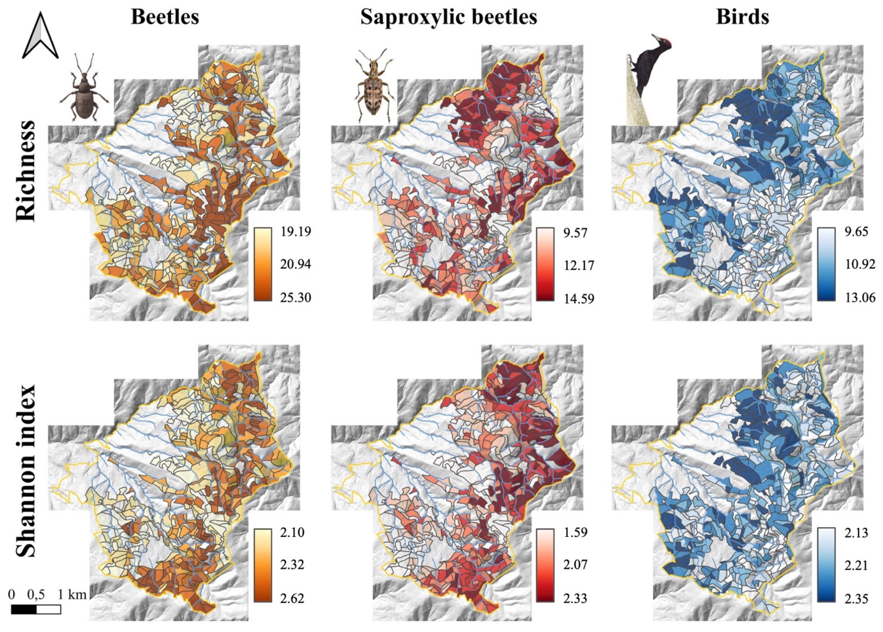
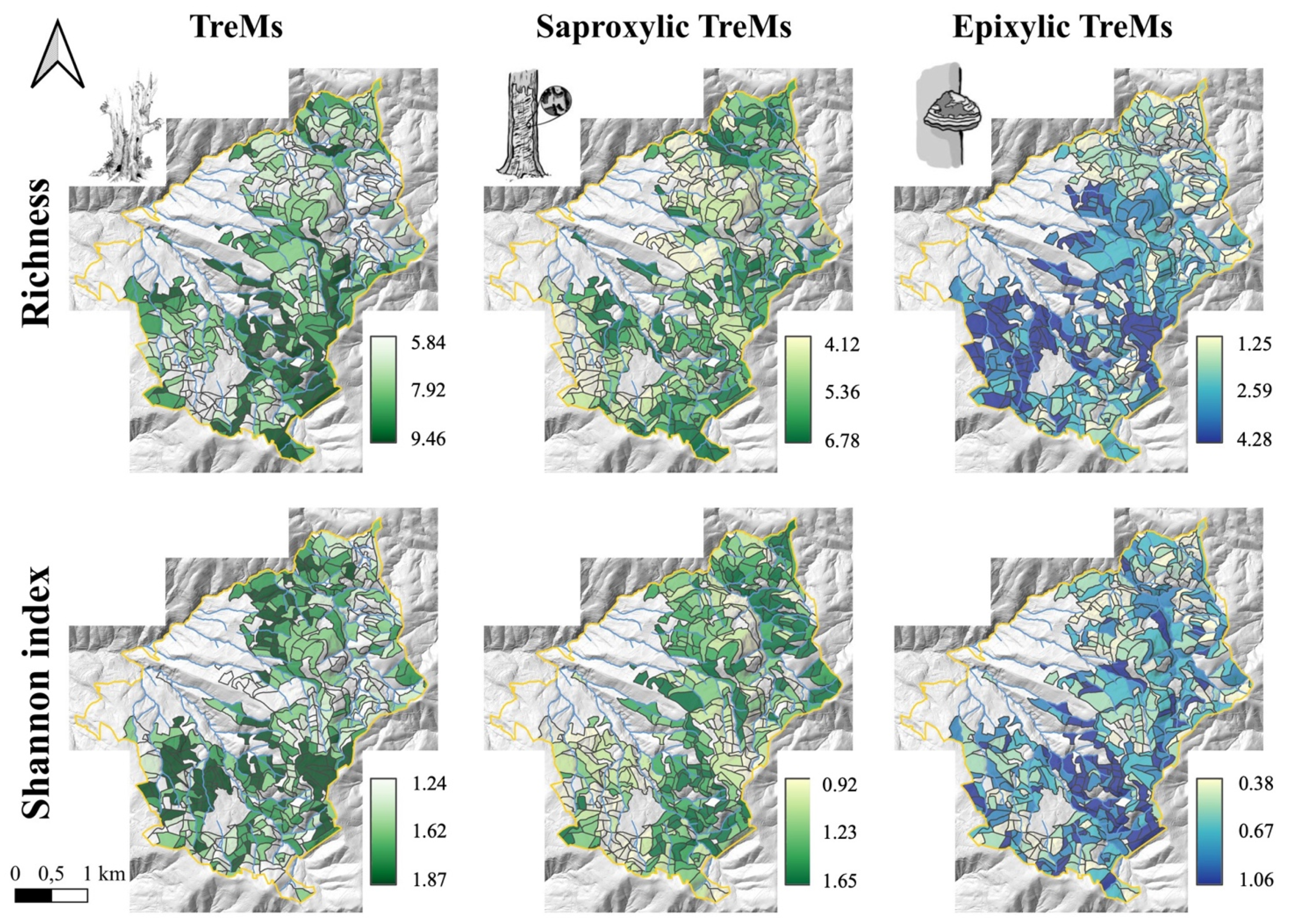
3.4. Random Forests Models and Maps of Biodiversity Indices

Results for the variable selection and validation of RF models are reported in Table 1 and in the Supplementary Material Table S5. After the variable selection, a maximum of seven and a minimum of two variables were selected as the best candidates for prediction. Overall, 26 unique variables were selected, 11 of which were selected in at least two models. The most selected variables were the point cloud-based ones: i. differences between 50 z percentiles of second intensity quartiles and 25 z percentiles of second intensity quartiles; ii. intensity skewness; and iii. the tenth z percentiles of fourth intensity quartiles and the slope (three models). Of the selected variables, eighteen were directly derived from the point cloud, four were derived from CHM (textural metrics), three were auxiliary variables, and one was an RGB metric derived from spectral reflectance.
The RMSE% of the final models ranged between 8.5 (birds’ Shannon index) and 50.2 (epixylic TreMs types’ Shannon index). On average, the Shannon index (20.9) was predicted to perform better than the richness (27.6), except for the epixylic TreMs, with an overall mean difference of −6.7%. Similarly, R2 was higher for the Shannon index (mean R2 = 0.17, against 0.14 for the richness).
Based on these models, the wall-to-wall maps of the richness and diversity of beetles, saproxylic beetles, birds, and microhabitats, both overall and divided into saproxylic and epixylic categories, were developed for the silver fir, beech, and mixed fir–beech stands of the Nature Reserve of Vallombrosa (Figure 2 and Figure 3).
Considering beetles, the richness map shows the highest values among all species and TreeM types assessed; values ranged between 19.2 and 25.3 (Figure 2), while for saproxylic beetles the richness was between 9.6 and 14.6 (Figure 2). Similar values were identified for birds, with the richness ranging between 9.7 and 13.1 (Figure 2). The Shannon index for beetles was between 2.1 and 2.6 (Figure 2), and slightly lower values were found for both saproxylic beetles (1.6–2.3) (Figure 2) and birds (2.1–2.3) (Figure 2).
As for the TreM maps, starting from the overall richness (TreMs), which varied between 5.8 and 9.5 (Figure 3), we found higher values for saproxylic TreMs (4.1–6.8) (Figure 3) compared to epixylic TreMs (1.2–4.3) (Figure 3). Concerning species diversity, the minimum value of the Shannon index for TreMs was 1.2, while the maximum was 1.9 (Figure 3). When the TreMs were split into two categories, the values were between 0.9 and 1.7 for saproxylic (Figure 3) and 0.3–1.1 for epixylic (Figure 3), respectively.

4. Discussion

4.1. Relationship between ALS Data and Multi-Taxon Biodiversity

In addition to studies of beetle and bird communities and TreMs distributions, ALS data hold great potential for analyzing the relationship between forest structure and animal diversity [31]. ALS-based approaches are, therefore, increasingly being used to explore, explain, and predict biodiversity given the promising results and replicability of procedures [5,35,59]. However, the relationship between ALS data and multi-taxon biodiversity has seldom been explored. In this context, we explored the relationship between taxa and ALS in the Nature Reserve of Vallombrosa, a Mediterranean mountainous forested area dominated by silver fir and beech.
In this study, several ALS predictors were calculated [47] which are crucial elements for explaining the occurrence and distribution of the examined taxa. However, the variable selection procedure for each prediction model shows that a limited number of metrics were the best predictors, highlighting that single metrics can explain most of the information provided by the ALS point cloud. Moreover, selecting RF model variables ensures that information retrieved from calculated ALS metrics contributes to uncorrelated information. The most frequent ALS predictor for multi-taxon biodiversity represented the vegetation (e.g., the point cloud-based factors: intensity skewness; 10th z percentiles of fourth intensity quartiles, and differences between 50 z percentiles of second intensity quartiles and 25 z percentiles of second intensity quartiles) and the terrain structure (slope) (Supplementary Material Table S5).
The most important ALS metrics are point-cloud-based (18 of the 26 selected metrics). Among the ALS metrics developed from the intensity pulse and the z values, the most promising are the different z percentiles of each intensity quartile (e.g., for the Shannon index of saproxylic beetles, birds, TreMs, and epixylic TreMs together with the richness of saproxylic and epixylic TreMs) and the structural indices derived from the differences in these (e.g., richness of beetles, birds, epixylic TreMs, and Shannon index of birds and saproxylic and epixylic TreMs). Particularly, the intensity distribution in quartiles (e.g., the richness of the birds), the 20th percentile of z distribution (e.g., for beetle Shannon index), the difference between maximum and minimum intensity values (e.g., for saproxylic TreMs), intensity skewness (e.g., saproxylic beetle richness) were selected (Table 1 and Supplementary Material Table S5). Considering the vertical structure of the forest and ALS metrics, the canopy layer is mainly represented by the proportion of pulse in the upper point cloud vertical layer (10th percentile of z distribution). Additionally, multiple ALS metrics referring to the lower forest layers were selected, such as the high intensity values (4th quartile) of ALS pulses in the lower layers of the point cloud (10th and 20th percentiles of z distribution) (Table S5). Although outside the study scope, these metrics appear to benefit studies investigating forest species diversity, on the one hand, and to detect the occurrence of shrubs or dead wood in the forest, on the other.
In addition to the point cloud predictors, four predictors derived from the CHM were selected: the variance of GLCM (TreMs Shannon index), the standard deviation of GLCM homogeneity (richness of saproxylic beetles), the standard deviation of GLCM mean (richness of saproxylic TreMs), and the standard deviation of GLCM variance (Shannon index of beetles) (Table 1 and Supplementary Material Table S5). In addition to a predictor from spectral values (maximum value of blue for the Shannon index of saproxylic beetles), the last three were derived from auxiliary variables. In particular, the growing stock volume (for TreMs and saproxylic TreMs richness) and the two topographic predictors, slope (Shannon index of TreMs and epixylic TreMs and TreMs richness) and aspect (saproxylic TreMs Shannon index), were selected (Supplementary Material Table S5).
The selected predictors were found in similar studies in which the most frequent explanatory ALS variables selected for the forest structural diversity identification were the coefficient of variation, standard deviation and skewness of ALS heights, canopy cover metrics, and percentiles of vegetation heights [60]. Similar to Herniman et al. [61], our results show that ALS metrics describing topography (slope and aspect) can contribute to the modeling of the biodiversity of TreMs. Therefore, when modeling biodiversity, it is advisable to integrate structural predictors of vegetation with terrain predictors available from ALS data.
While promising, the results show a relatively low coefficient of determination (R2) (maximum 0.30) across all taxa and diversity indices. This can be caused by several factors, such as the complex non-linear relationship between predictors and diversity indices, the presence of outliers both in dependent and independent variables, the complexity of the model after the variable selection, and the low variability of diversity indices within the study area. However, our results in modeling species diversity indices are consistent with other, similar studies showing moderate results with values between 0 and 0.34 [31]. These values can be explained considering that the study area, while sufficiently large, has low environmental variability [62], and vegetation variations resulting in stronger correlations between ALS predictors and taxa [33]. In this sense, increasing the number of sampling areas could improve the results. Despite the low variance explained by the models, random forests obtained a high prediction accuracy, resulting in low RMSE values. Moreover, the aggregation of pixel predictions within homogeneous areas, such as the management units identified by the Reserve management plan, resulted in a close estimate of the true value as the aggregation area increased.
In the context of a forest management approach aimed at sustaining or increasing forest complexity and diversity, ALS, capable of investigating forest structure, emerges as a promising technique for extensively detecting and monitoring potential biodiversity hotspots over large areas [31].

4.2. Multi-Taxon Biodiversity and Forest Management

Our results show that specific habitat features (e.g., the occurrence of TreMs) are necessary in making forests suitable for beetle and bird communities. Furthermore, specific characteristics of forest areas may represent the entire species community. For example, saproxylic beetles are highly dependent on the microclimatic conditions of particular TreMs [14,63]. A knowledge of biodiversity indicators allows us to design and optimize management strategies that consider the particular ecological needs of some species of birds and beetles [64,65]. Specifically, our analysis could be used to identify some management options to preserve beetle and bird communities, promote tree habitats, increase total tree volume, and reduce overall forest density [66]. These characteristics are typical of mature forests, the achievement of which should be one of the objectives of sustainable forest management. However, the community structure of beetles and birds was not determined by habitat type, as the forest sectors considered were quite similar in fauna and vegetation [45,65].
Mixed forests with heterogeneous stands provide a greater ecological niche [62]. Forest management can have implications on the proportion of tree species, like, for example, the abandonment of silvicultural activities in mixed stands, which has led to an increase in beech and a decrease in silver fir [67]. On the other hand, in the Vallombrosa pure even-aged fir forests, where silvicultural practices have long been absent, gaps are spontaneously opening up with a gradual transformation into mixed, naturally regenerating forests. The management plan in place simulates these natural events to increase the specific diversity and structural and compositional complexity of the fir stands [38].

4.3. Biodiversity Conservation

The diversity of species and taxa sampled in this work is reflected in their different ecological roles and characteristics within the community, as well as in forest management. Notably, the relationship between the different analyzed taxa and the tree component depends on the trees’ physical structure, which can be derived from ALS point clouds through 3D structural metrics. Large trees with complex canopy structures are often cavitated and rich in TreMs, hosting populations of saproxylic beetle communities and birds. Moreover, the high number of different TreMs typically found in long-unmanaged stands results in differential levels of specialization of the ornithic and saproxylic components, often at risk of extinction [8,14]. As for the Picidae, Bütler et al. [68] have suggested conserving at least 5% of standing dead trees in forest areas larger than 100 ha. These thresholds correspond to the amount of habitat below which fragmentation may affect population persistence [69].
About half of the sampled beetles in the forest of Vallombrosa are saproxylic species included in the Italian Red List. Saproxylic beetles include highly specialized species. Consequently, they are considered valid indicators for assessing the naturalness of forest ecosystems [21]. In our case, we found 10 endangered species, including Megathous nigerrimus (Elateridae) and Anaspis ruficollis (Scraptiidae) for the Endangered (EN) category and Mordellochroa milleri (Mordellidae) included in the Critically Endangered (CR) category. Furthermore, two species were included in the DD (Data Deficient) category (i.e., Rhizophagus cribratus and R. perforatus (Monotomidae)). Saproxylic beetles play an essential role in the food chain of the forest ecosystem, particularly in the recycling of nutrients, as they depend on—or are involved in—deadwood decay processes. However, information on the status and distribution of the population of these species is particularly scarce in the Mediterranean area [70]. Our results indicate that vertical forest heterogeneity is an important variable for saproxylic assemblages in these Mediterranean montane forests [14].
In the Northern Apennines (including the study area), the presence of a significant proportion of conifers is a decisive factor for the occurrence of numerous bird species [65], including, among the target species, Lophophanes cristatus and the Dryocopus martius [71]. Mixed forests generally have heterogeneous stands, providing a greater range of nesting and foraging sites [72,73]. Indeed, cavity-nesting species, being more vulnerable to mammalian predation, could therefore suffer from the indirect effect of an increase in tree species [74]. Species that have specific habitat requirements (e.g., the presence of cavities, the structure of canopy layers) usually have strict preferences in terms of tree species, and therefore an increase in tree species in general could correspond to a decrease in the availability of niches [72].

4.4. ALS Data, Limitations, and Opportunities

ALS data represent an effective technique for detecting multi-taxon biodiversity patterns. They can be used at different spatial scales to capture highly detailed data about forest structure and terrain characteristics, also facilitating monitoring purposes thanks to easy comparability when a multitemporal survey is available. Despite the excellent opportunities remote sensing offers, some limitations must also be considered. Although ALS data provide information at the level of the canopy and its structure [75], in dense and continuously closed canopies, ALS metrics cannot fully describe the ecosystem biodiversity by capturing microspatial variations [62], for which accurate field campaigns remain necessary. Accordingly, one potential issue of ALS is related to the point density. Specifically, as the density of points decreases, the forest structure ALS variables become less accurate. Particularly promising are high-point-density ALS data that allow detailed descriptions of lower canopy structures and enable new voxel-based approaches to retrieve information from ALS data [76]. On the other hand, our ALS metrics are derived from a survey at 10 pulses m−2, which is higher than other studies that still showed reasonable results (<2 pulses m−2) [31].
Furthermore, ALS data can provide a snapshot of the landscape at a specific time, while biodiversity is dynamic. Due to the acquisition cost, ALS data are often not open access and cannot provide repeated and temporally dense observations, not capturing seasonal variations, migration patterns, or long-term trends. Moreover, and most critical, is the lack of national wall-to-wall ALS data in many countries, as in Italy, which limits large-scale implementation [49,52].
On the other hand, RS data are repeatable and increasingly freely accessible and can be used at different spatial and temporal scales to support fieldwork limitations [77]. Accordingly, combining field activities and remote sensing approaches (also considering integration with other RS spectral data) for forest monitoring can overcome these shortcomings, helping to design and optimize regular and cost-effective monitoring strategies to address biodiversity loss in forest ecosystems. Therefore, further biodiversity studies should be conducted to evaluate the effectiveness of satellite LiDAR data such as GEDI [78], or the integration with terrestrial laser scanning data, to overcome the major limitations of ALS in penetrating the canopy in dense forests. On the other hand, RS data do not replace field surveys, which are essential for assessing forest biodiversity and identifying individual species, along with their rarity and composition.
Furthermore, TreMs are not the only drivers of ecological indicators of habitats for animal species, which are also determined by multiple interspecific and intraspecific biotic interactions with forest variables [14]. Therefore, our integrated approach could help in identifying hotspots in the forest with the greatest need for management interventions to improve the conservation of red-listed saproxylic species and birds.
We believe that processing and analyzing such data, which also allows the detailed mapping of forest variables, including biodiversity indices, will be essential tools that have the potential to support conservation planning and decision-making in forest ecosystems.

5. Conclusions

The following conclusions can be drawn from our study:
(1)
ALS data hold great potential for analyzing the relationship between forest structure and saproxylic and non-saproxylic beetle and bird communities. Forest structure and TreMs were the most important variables in determining the multi-taxon biodiversity in Mediterranean mountain ecosystems. Thus, accurate data on forest structure and microhabitat-type indicators emerged as crucial for forest management and biodiversity conservation.
(2)
Remote sensing provides powerful tools to study the diversity and abundance of forest biodiversity indicators (i.e., insects, birds, and TreMs). The large availability of data at different spatial and temporal resolutions allows saproxylic beetle and bird communities to be investigated at the most appropriate scale to discover new ecological, ethological, and conservation information.
(3)
Currently, ALS data can capture information on the composition and structure of ecologically suitable habitats for animal species. Habitat resources (trophic niches—TreMs) can be distinguished using the variables obtainable from point clouds. Furthermore, the different biodiversity conditions detected with the ground surveys were mapped at physiologically relevant scales for insects and birds.
(4)
In the near future, remote sensing will be increasingly used for specific indicators of forest biodiversity. Although limitations for fully successful implementation are still emerging, technological progress will make it possible to obtain information on threatened species, thus informing nature-based forest management.
(5)
In future studies, we suggest including other taxonomic groups related to forest structural traits (e.g., small mammals, spiders, amphibians, lichens, fungi, and bryophytes). This will ensure the comprehensive monitoring of forest ecosystems to identify biodiversity hotspots more effectively.
(6)
Multi-taxon biodiversity data permit the definition and strengthening of sustainable management indicators linked to the different functions in forest ecosystems. This is useful for drawing implications for conservation strategies of forest environments and for increasing the resilience of mountain forests threatened by climate change.

Supplementary Materials

The following supporting information can be downloaded at: https://www.mdpi.com/article/10.3390/f15040660/s1, Table S1: Groups and forms of Tree-related microhabitat types, according to Kraus et al. [46] Table S2: Summary of the ALS metrics, according to Giannetti et al. [47]; Table S3: List of the saproxylic and non-saproxylic beetle species sampled in the Nature Reserve of Vallombrosa; Table S4: List of the birds species identified in the Nature Reserve of Vallombrosa; Table S5: Results of the variable selection.

Author Contributions

Conceptualization, Data curation, Investigation, Methodology, Resources, Roles/Writing—original draft, Writing—review and editing, F.P. and G.D.; Resources, Roles/Writing—original draft, Writing—review and editing, E.V., S.F., C.C., F.G., G.L., S.N., C.B., G.C. and D.T.; Supervision; Writing—review and editing. All authors have read and agreed to the published version of the manuscript.

Funding

This study was partially supported by the following projects: PNRR, project funded under the National Recovery and Resilience Plan (NRRP), Mission 4 Component 2 Investment 1.4—Call for tender No. 3138 of 16 December 2021, rectified by Decree n.3175 of 18 December 2021 of the Italian Ministry of University and Research funded by the European Union—NextGenerationEU; Project code CN_00000033, Concession Decree No. 1034 of 17 June 2022 adopted by the Italian Ministry of Universities and Research, CUP H73C22000300001, Project title “National Biodiversity Future Center—NBFC”.

Data Availability Statement

The data presented in this study are available upon request from the corresponding author.

Acknowledgments

The authors thank the specialists of the various taxonomic groups: Paolo Audisio (Nitidulidae), Enzo Colonnelli (Curculionidae), Davide Vallotto (Curculionidae Scolytinae), Gianluca Magnani (Buprestidae), Gianfranco Liberti (Melyridae), Giuseppe Platia (Elateridae), Fabrizio Fanti (Cantharidae, Lampyridae), Emanuele Piattella (Scarabaeidae), Pierpaolo Rapuzzi (Cerambycidae (pars)), Enrico Ruzzier (Scraptiidae, Mordellidae), Gianfranco Salvato (Biphyllidae, Mycetophagidae (pars), Zopheridae (pars)), Adriano Zanetti (Staphylinidae (pars)). In addition, we wish to thank the Reparto Carabinieri Biodiversità di Vallombrosa for their logistical support during the fieldwork.

Conflicts of Interest

The authors declare no conflicts of interest.

References

  1. FAO. State of the World’s Forests. Food and Agriculture Organization of the United Nations; FAO: Rome, Italy, 2012. [Google Scholar]
  2. Trentanovi, G.; Campagnaro, T.; Sitzia, T.; Chianucci, F.; Vacchiano, G.; Ammer, C.; Ciach, M.; Nagel, T.A.; del Río, M.; Paillet, Y.; et al. Words apart: Standardizing forestry terms and definitions across European biodiversity studies. For. Ecosyst. 2023, 10, 100128. [Google Scholar] [CrossRef]
  3. Oettel, J.; Lapin, K. Linking forest management and biodiversity indicators to strengthen sustainable forest management in Europe. Ecol. Indic. 2021, 122, 107275. [Google Scholar] [CrossRef]
  4. Leitão, P.J.; Toraño Caicoya, A.; Dahlkamp, A.; Guderjan, L.; Griesser, M.; Haverkamp, P.J.; Nordén, J.; Snäll, T.; Schröder, B. Impacts of Forest Management on Forest Bird Occurrence Patterns—A Case Study in Central Europe. Front. For. Glob. Chang. 2022, 5, 786556. [Google Scholar] [CrossRef]
  5. Kõrkjas, M.; Remm, L.; Lõhmus, P.; Lõhmus, A. From tree-related microhabitats to ecosystem management: A tree-scale investigation in productive forests in Estonia. J. Environ. Manag. 2023, 343, 118245. [Google Scholar] [CrossRef] [PubMed]
  6. Munro, N.T.; Fischer, J.; Barrett, G.; Wood, J.; Leavesley, A.; Lindenmayer, D.B.B. Bird’s response to revegetation of different structure and floristics e are “restoration plantings” restoring bird communities? Restor. Ecol. 2010, 19, 223–235. [Google Scholar] [CrossRef]
  7. Bae, S.; Müller, J.; Lee, D.; Vierling, K.T.; Vogeler, J.C.; Vierling, L.A.; Hudak, A.T.; Latifi, H.; Thorn, S. Taxonomic, functional, and phylogenetic diversity of bird assemblages are oppositely associated to productivity and heterogeneity in temperate forests. Remote Sens. Environ. 2018, 215, 145–156. [Google Scholar] [CrossRef]
  8. Campanaro, A.; Parisi, F. Open datasets wanted for tracking the insect decline: Let’s start from saproxylic beetles. Biodivers. Data J. 2021, 9, e72741. [Google Scholar] [CrossRef]
  9. Bunce, R.G.H.; Bogers, M.M.B.; Evans, D.; Halada, L.; Jongman, R.H.G.; Mucher, C.A.; Bauch, B.; de Bluste, G.; Parr, T.W.; Olsvig-Whittaker, L. The significance of habitats as indicators of biodiversity and their links to species. Ecol. Indic. 2013, 33, 19–25. [Google Scholar] [CrossRef]
  10. Lachat, T.; Wermelinger, B.; Gossner, M.M.; Bussler, H.; Isacsson, G.; Müller, J. Saproxylic beetles as indicator species for deadwood amount and temperature in European beech forests. Ecol. Indic. 2012, 23, 323–331. [Google Scholar] [CrossRef]
  11. Ram, D.; Axelsson, A.L.; Green, M.; Smith, H.G.; Lindström, Å. What drives current population trends in forest birds–forest quantity, quality or climate? A large-scale analysis from northern Europe. For. Ecol. Manag. 2017, 385, 177–188. [Google Scholar] [CrossRef]
  12. Roberge, J.; Angelstam, P. Indicator species among resident forest birds A cross-regional evaluation in northern Europe. Biol. Conserv. 2006, 130, 134–147. [Google Scholar] [CrossRef]
  13. Nadkarni, N.M.; McIntosh, A.C.; Cushing, J.B. A framework to categorize forest structure concepts. Forest Ecol. Manag. 2008, 256, 872–882. [Google Scholar] [CrossRef]
  14. Spina, P.; Parisi, F.; Antonucci, S.; Garfì, V.; Marchetti, M.; Santopuoli, G. Tree-related microhabitat diversity as a proxy for the conservation of beetle communities in managed forests of Fagus sylvatica. For. Int. J. For. Res. 2023, 97, 223–233. [Google Scholar] [CrossRef]
  15. Vergara, P.M.; Fierro, A.; Carvajal, M.A.; Alaniz, A.J.; Quiroz, M. Multiple environmental drivers for the Patagonian forest-dwelling beetles: Contrasting functional and taxonomic responses across strata and trophic guilds. Sci. Total Environ. 2022, 838, 155906. [Google Scholar] [CrossRef] [PubMed]
  16. Blondel, J. Origins and dynamics of forest birds of the northern hemisphere. In Ecology and Conservation of Forest Birds; Mikusinski, G., Roberge, J.M., Fuller, R.J., Eds.; Cambridge University Press: Cambridge, UK, 2018; pp. 11–50. [Google Scholar] [CrossRef]
  17. Kriegel, P.; Vogel, S.; Angeleri, R.; Baldrian, P.; Borken, W.; Bouget, C.; Brin, A.; Bussler, H.; Cocciufa, C.; Feldmann, B.; et al. Ambient and substrate energy influence decomposer diversity differentially across trophic levels. Ecol. Lett. 2023, 26, 1157–1173. [Google Scholar] [CrossRef] [PubMed]
  18. Gregory, R.D.; Van Strien, A.; Vorisek, P.; Gmelig Meyling, A.W.; Noble, D.G.; Foppen, R.P.; Gibbons, D.W. Developing indicators for European birds. Philos. Trans. R. Soc. B Biol. Sci. 2005, 360, 269–288. [Google Scholar] [CrossRef] [PubMed]
  19. Storch, F.; Boch, S.; Gossner, M.M.; Feldhaar, H.; Ammer, C.; Schall, P.; Polle, A.; Kroiher, F.; Muller, J.; Bauhus, J. Linking structure and species richness to support forest biodiversity monitoring at large scales. Ann. For. Sci. 2023, 80, 3. [Google Scholar] [CrossRef]
  20. Hanle, J.; Duguid, M.C.; Ashton, M.S. Legacy forest structure increases bird diversity and abundance in aging young forests. Ecol. Evol. 2020, 10, 1193–1208. [Google Scholar] [CrossRef]
  21. Carpaneto, G.M.; Baviera, C.; Biscaccianti, A.B.; Brandmayr, P.; Mazzei, A.; Mason, F.; Battistoni, A.; Teofili, C.; Rondinini, C.; Fattorini, S.; et al. A Red List of Italian Saproxylic Beetles: Taxonomic overview, ecological features and conservation issues (Coleoptera). Fragm. Entomol. 2015, 47, 53–126. [Google Scholar] [CrossRef]
  22. Culbert, P.D.; Radeloff, V.C.; Flather, C.H.; Kellndorfer, J.M.; Rittenhouse, C.D.; Pidgeon, A.M. The influence of vertical and horizontal habitat structure on nationwide patterns of avian biodiversity. Ornithology 2013, 130, 656–665. [Google Scholar] [CrossRef]
  23. Gustin, M.; Nardelli, R.; Brichetti, P.; Battistoni, A.; Rondinini, C.; Teofili, C. Lista Rossa IUCN degli uccelli nidificanti in Italia. In Comitato Italiano IUCN e Ministero dell’Ambiente e della Tutela del Territorio e del Mare; Ufficio federale dell’ambiente (UFAM): Berna, Switzerland; Stazione ornitologica svizzera: Sempach, Switzerland, 2021. [Google Scholar]
  24. Lindén, S.F.A.; Lehikoinen, A. Population trends of common breeding forest birds in southern Finland are consistent with trends in forest management and climate change. Ornis Fenn. 2015, 92, 187–203. [Google Scholar]
  25. Vogeler, J.C.; Hudak, A.T.; Vierling, L.A.; Evans, J.; Green, P.; Vierling, K.T. Terrain and vegetation structural influences on local avian species richness in two mixed-conifer forests. Remote Sens. Environ. 2014, 147, 13–22. [Google Scholar] [CrossRef]
  26. Clawges, R.; Vierling, K.; Vierling, L.; Rowell, E. The use of airborne lidar to assess avian species diversity, density, and occurrence in a pine/aspen forest. Remote Sens. Environ. 2008, 112, 2064–2073. [Google Scholar] [CrossRef]
  27. Jacobsen, R.M.; Sverdrup-Thygeson, A.; Birkemoe, T. Scale-specific responses of saproxylic beetles: Combining dead wood surveys with data from satellite imagery. J. Insect Conserv. 2015, 19, 1053–1062. [Google Scholar] [CrossRef]
  28. Martinuzzi, S.; Vierling, L.A.; Gould, W.A.; Falkowski, M.J.; Evans, J.S.; Hudak, A.T.; Vierling, K.T. Mapping snags and understory shrubs for a LiDAR-based assessment of wildlife habitat suitability. Remote Sens. Environ. 2009, 113, 2533–2546. [Google Scholar] [CrossRef]
  29. Zhang, J.; Huang, Y.; Pu, R.; Gonzalez-Moreno, P.; Yuan, L.; Wu, K.; Huang, W. Monitoring plant diseases and pests through remote sensing technology: A review. Comput. Electron. Agric. 2019, 165, 104943. [Google Scholar] [CrossRef]
  30. Filho, F.H.I.; Heldens, W.B.; Kong, Z.; de Lange, E.S. Drones: Innovative technology for use in precision pest management. J. Econ. Entomol. 2020, 113, 1–25. [Google Scholar] [CrossRef] [PubMed]
  31. Toivonen, J.; Kangas, A.; Maltamo, M.; Kukkonen, M.; Packalen, P. Assessing biodiversity using forest structure indicators based on airborne laser scanning data. For. Ecol. Manag. 2023, 546, 121376. [Google Scholar] [CrossRef]
  32. Galbraith, S.M.; Vierling, L.A.; Bosque-Perez, N.A. Remote sensing and ecosystem services: Current status and future opportunities for the study of bees and pollination-related services. Curr. For. Rep. 2015, 1, 261–274. [Google Scholar] [CrossRef]
  33. Rada, P.; Padilla, A.; Horák, J.; Micó, E. Public LiDAR data are an important tool for the detection of saproxylic insect hotspots in Mediterranean forests and their connectivity. For. Ecol. Manag. 2022, 520, 120378. [Google Scholar] [CrossRef]
  34. Kane, V.R.; McGaughey, R.J.; Bakker, J.D.; Gersonde, R.F.; Lutz, J.A.; Franklin, J.F. Comparisons between field- and LiDAR-based measures of stand structural complexity. Can. J. For. Res. 2010, 40, 761–773. [Google Scholar] [CrossRef]
  35. Müller, J.; Bae, S.; Röder, J.; Chao, A.; Didham, R.K. Airborne LiDAR reveals context dependence in the effects of canopy architecture on arthropod diversity. For. Ecol. Manag. 2014, 312, 129–137. [Google Scholar] [CrossRef]
  36. Bombi, P.; Gnetti, V.; D’Andrea, E.; De Cinti, B.; Vigna Taglianti, A.; Bologna, M.A.; Matteucci, G. Identifying priority sites for insect conservation in forest ecosystems at high resolution: The potential of LiDAR data. J. Insect Conserv. 2019, 23, 689–698. [Google Scholar] [CrossRef]
  37. North, M.P.; Kane, J.T.; Kane, V.R.; Asner, G.P.; Berigan, W.; Churchill, D.J.; Conway, S.; Gutiérrez, R.J.; Jeronimo, S.; Keane, J.; et al. Cover of tall trees best predicts California spotted owl habitat. For. Ecol. Manag. 2017, 405, 166–178. [Google Scholar] [CrossRef]
  38. Bottalico, F.; Travaglini, D.; Fiorentini, S.; Lisa, C.; Nocentini, S. Stand dynamics and natural regeneration in silver fir (Abies alba Mill.) plantations after traditional rotation age. iForest 2014, 7, 313–323. [Google Scholar] [CrossRef]
  39. Ciancio, O. Riserva Naturale Statale Biogenetica di Vallombrosa. Piano di Gestione e Silvomuseo 2006–2025; Corpo Forestale dello Stato, Ufficio Territoriale per la Biodiversità di Vallombrosa, Reggello (FI): Florence, Italy, 2009; pp. 113–134. ISBN 978-88-87553-17-8. [Google Scholar]
  40. Nocentini, S.; Ciancio, O.; Portoghesi, L.; Corona, P. Historical roots and the evolving science of forest management under a systemic perspective. Can. J. For. Res. 2021, 51, 163–171. [Google Scholar] [CrossRef]
  41. QGIS.org. QGIS Geographic Information System. 2024, QGIS Association. Available online: http://www.qgis.org (accessed on 2 January 2024).
  42. Bouchard, P.; Bousquet, Y.; Davies, A.E.; Alonso-Zarazaga, M.A.; Lawrence, J.F.; Lyal, C.H.C.; Newton, A.F.; Reid, C.A.M.; Schmitt, M.; Slipinski, S.A.; et al. Family-group names in Coleoptera (Insecta). ZooKeys 2011, 88, 1–972. [Google Scholar]
  43. Audisio, P.; Zarazaga, M.A.; Slipinski, A.; Nilsson, A.; Jelínek, J.; Taglianti, A.V.; Turco, F.; Otero, C.; Canepari, C.; Kral, D.; et al. Fauna Europaea: Coleoptera 2 (excl. series Elateriformia, Scarabaeiformia, Staphyliniformia and superfamily Curculionoidea). Biodivers. Data J. 2015, 3, e4750. [Google Scholar] [CrossRef]
  44. Bibby, C.J.; Burgess, N.D.; Hillis, D.M.; Hill, D.A.; Mustoe, S. Bird Census Techniques, 2nd ed; Academic Press: London, UK, 2000; ISBN 9780120958313. [Google Scholar]
  45. Baccetti, N.; Fracasso, G. CISO-COI Check-list of Italian birds-2020. Avocetta 2021, 45, 21–82. [Google Scholar]
  46. Kraus, D.; Bütler, R.; Krumm, F.; Lachat, T.; Larrieu, L.; Mergner, U.; Paillet, Y.; Rydkvist, T.; Schuck, A.; Winter, S. Catalogue of Tree Microhabitats—Reference Field List Integrate + Technical Paper; European Forest Insitute: Freiburg, Germany, 2006; 16p. [Google Scholar]
  47. Giannetti, F.; Chirici, G.; Gobakken, T.; Naesset, E.; Travaglini, D.; Puliti, S. A new approach with DTM-independent metrics for forest growing stock prediction using UAV photogrammetric data. Remote Sens. Environ. 2018, 213, 195–205. [Google Scholar] [CrossRef]
  48. Michałowska, M.; Rapiński, J. A Review of Tree Species Classification Based on Airborne LiDAR Data and Applied Classifiers. Remote Sens. 2021, 13, 353. [Google Scholar] [CrossRef]
  49. Gschwantner, T.; Alberdi, I.; Bauwens, S.; Bender, S.; Borota, D.; Bosela, M.; Bouriaud, O.; Breidenbach, J.; Donis, J.; Fischer, C.; et al. Growing stock monitoring by European National Forest Inventories: Historical origins, current methods and harmonisation. For. Ecol. Manag. 2022, 505, 119868. [Google Scholar] [CrossRef]
  50. Laes, D.; Reutebuch, S.E.; McGaughey, R.J.; Mitchell, B. Guidelines to Estimate Forest Inventory Parameters from LiDAR and Field Plot Data; Companion document to the Advanced Lidar Applications; U.S. Department of Agriculture Forest Service: Washington, DC, USA, 2011.
  51. Næsset, E. Practical large-scale forest stand inventory using a small-footprint airborne scanning laser. Scand. J. For. Res. 2004, 19, 164–179. [Google Scholar] [CrossRef]
  52. Vangi, E.; D’Amico, G.; Francini, S.; Borghi, C.; Giannetti, F.; Corona, P.; Marchetti, M.; Travaglini, D.; Pellis, G.; Vitullo, M.; et al. Large-scale high-resolution yearly modeling of forest growing stock volume and above-ground carbon pool. Environ. Model. Softw. 2023, 159, 105580. [Google Scholar] [CrossRef]
  53. Breidenbach, J.; Waser, L.T.; Debella-Gilo, M.; Schumacher, J.; Rahlf, J.; Hauglin, M.; Puliti, S.; Astrup, R. National mapping and estimation of forest area by dominant tree species using Sentinel-2 data. Can. J. For. Res. 2021, 51, 365–379. [Google Scholar] [CrossRef]
  54. Breiman, L. Random Forests. Mach. Learn. 2001, 45, 5–32. [Google Scholar] [CrossRef]
  55. Genuer, R.; Poggi, J.M.; Tuleau-Malot, C. VSURF: An R package for variable selection using random forests. R J. 2015, 7, 19–33. [Google Scholar] [CrossRef]
  56. R Core Team. R: A Language and Environment for Statistical Computing; R Foundation for Statistical Computing: Vienna, Austria, 2022; Available online: https://www.R-project.org (accessed on 2 January 2024).
  57. Wright, M.N.; Ziegler, A. Ranger: A fast implementation of random forests for high dimensional data in C++ and R. J. Stat. Softw. 2017, 77, 1–17. [Google Scholar] [CrossRef]
  58. Chen, F.; Hou, Z.; Saarela, S.; McRoberts, R.E.; Ståhl, G.; Kangas, A.; Packalen, P.; Li, B.; Xu, Q. Leveraging remotely sensed non-wall-to-wall data for wall-to-wall upscaling in forest inventory. Int. J. Appl. Earth Obs. Geoinf. 2023, 119, 103314. [Google Scholar] [CrossRef]
  59. Ćosović, M.; Bugalho, M.N.; Thom, D.; Borges, J.G. Stand Structural Characteristics Are the Most Practical Biodiversity Indicators for Forest Management Planning in Europe. Forests 2020, 11, 343. [Google Scholar] [CrossRef]
  60. Dalponte, M.; Ene, L.T.; Gobakken, T.; Næsset, E.; Gianelle, D. Predicting selected forest stand characteristics with multispectral ALS data. Remote Sens. 2018, 10, 586. [Google Scholar] [CrossRef]
  61. Herniman, S.; Coops, N.C.; Martin, K.; Thomas, P.; Luther, J.E.; van Lier, O.R. Modelling avian habitat suitability in boreal forest using structural and spectral remote sensing data. Remote Sens. Appl. Soc. Environ. 2020, 19, 100344. [Google Scholar] [CrossRef]
  62. Rooney, R.C.; Azeria, E.T. The strength of cross-taxon congruence in species composition varies with the size of regional species pools and the intensity of human disturbance. J. Biogeogr. 2015, 42, 439–451. [Google Scholar] [CrossRef]
  63. Hammond, M.E.; Pokorný, R.; Okae-Anti, D.; Gyedu, A.; Obeng, I.O. The composition and diversity of natural regeneration of tree species in gaps under different intensities of forest disturbance. J. For. Res. 2021, 32, 1843–1853. [Google Scholar] [CrossRef]
  64. Grove, S.J. Saproxylic insect ecology and the sustainable management of forests. Annu. Rev. Ecol. Syst. 2002, 33, 1–23. [Google Scholar] [CrossRef]
  65. Martini, I.; Galipò, G.; Foderi, C.; Tocci, R.; Sargentini, C. Ornithical community of Vallombrosa Biogenetic National Nature Reserve (Italy). Eur. Zool. J. 2021, 88, 254–268. [Google Scholar] [CrossRef]
  66. Lange, M.; Türke, M.; Pašalić, E.; Boch, S.; Hessenmöller, D.; Müller, J.; Prati, D.; Socher, S.A.; Fischer, M.; Weisser, W.W.; et al. Effects of forest management on ground-dwelling beetles (Coleoptera; Carabidae, Staphylinidae) in Central Europe are mainly mediated by changes in forest structure. For. Ecol. Manag. 2014, 329, 166–176. [Google Scholar] [CrossRef]
  67. Sitzia, T.; Piazzi, C.; Barazzutti, G.; Campagnaro, T. Abandonment of timber harvesting favours European beech over silver fir: Evidence from Val Tovanella Nature Reserve in the southern Dolomites (Northern Italy). J. Prot. Mt. Areas Res. Manag. 2018, 10, 17–27. [Google Scholar] [CrossRef]
  68. Bütler, R.; Angelstam, P.; Ekelund, P.; Schlaeffer, R. Dead wood threshold values for the three-toed woodpecker presence in boreal and sub-Alpine forest. Biol. Conserv. 2004, 119, 305–318. [Google Scholar] [CrossRef]
  69. Fahrig, L. When does fragmentation of breeding habitat affect population survival? Ecol. Model. 1998, 105, 273–292. [Google Scholar] [CrossRef]
  70. García, N.; Numa, C.; Bartolozzi, L.; Brustel, H.; Buse, J.; Norbiato, M.; Recalde, J.I.; Zapata, J.; Dodelin, B.; Alcázar, E.; et al. The Conservation Status and Distribution of Mediterranean Saproxylic Beetles; IUCN: Gland, Switzerland, 2019. [Google Scholar] [CrossRef]
  71. Tellini Florenzano, G.; Cutini, S.; Campedelli, T.; Londi, G. Ecology and possible evolution of Crested Tit (Lophophanes cristatus) and Black Woodpecker (Dryocopus martius) populations in the Apennines, Italy. In Proceedings of the Bird Numbers 2010 “Monitoring, Indicators and Targets”. Book of Abstracts of the 18th Conference of the European Bird Census Council, Cáceres, Spain, 22–26 March 2010; Bermejo, A., Ed.; SEO/BirdLife: Madrid, Spain, 2010; p. 119. [Google Scholar]
  72. Batáry, P.; Fronczek, S.; Normann, C.; Scherber, C.; Tscharntke, T. How do edge effect and tree species diversity change bird diversity and avian nest survival in Germany’s largest deciduous forest? For. Ecol. Manag. 2014, 319, 44–50. [Google Scholar] [CrossRef]
  73. Wesolowski, T.; Fuller, R.J.; Flade, M. Temperate forests. A European perspective on variation and dynamics in bird assemblages. In Ecology and Conservation of Forest Birds; Mikusinski, G., Roberge, J.M., Fuller, R.J., Eds.; Cambridge University Press: Cambridge, UK, 2018. [Google Scholar]
  74. Wesolowski, T.; Martin, K. Tree holes and hole-nesting birds in European and North-American forests. In Ecology and Conservation of Forest Birds; Mikusinski, G., Roberge, J.M., Fuller, R.J., Eds.; Cambridge University Press: Cambridge, UK, 2018. [Google Scholar]
  75. Coops, N.C.; Tompalski, P.; Goodbody, T.R.; Queinnec, M.; Luther, J.E.; Bolton, D.K.; White, J.C.; Wulder, M.A.; van Lier, O.R.; Hermosilla, T. Modelling lidar-derived estimates of forest attributes over space and time: A review of approaches and future trends. Remote Sens. Environ. 2021, 260, 112477. [Google Scholar] [CrossRef]
  76. Sasaki, T.; Imanishi, J.; Fukui, W.; Morimoto, Y. Fine-scale characterization of bird habitat using airborne LiDAR in an urban park in Japan. Urban For. Urban Green. 2016, 17, 16–22. [Google Scholar] [CrossRef]
  77. Cerrejón, C.; Valeria, O.; Mansuy, N.; Barbé, M.; Fenton, N.J. Predictive mapping of bryophyte richness patterns in boreal forests using species distribution models and remote sensing data. Ecol. Indic. 2020, 119, 106826. [Google Scholar] [CrossRef]
  78. Dubayah, R.; Blair, J.B.; Goetz, S.; Fatoyinbo, L.; Hansen, M.; Healey, S.; Hofton, M.; Hurtt, G.; Kellner, J.; Luthcke, S. The Global Ecosystem Dynamics Investigation: High-resolution laser ranging of the Earth’s forests and topography. Sci. Remote Sens. 2020, 1, 100002. [Google Scholar] [CrossRef]
Figure 2. Biodiversity maps for silver fir, beech and mixed fir–beech stands. Richness (top) and diversity (bottom) of beetle, saproxylic beetle, and bird species. Values are the mean of pixel values within each stand.
Forests 15 00660 g002
Figure 3. Biodiversity maps for silver fir, beech and mixed fir–beech stands. Richness (top) and diversity (bottom) of TreM types for saproxylic and epixylic TreMs. Values are the mean of pixel values within each stand.
Forests 15 00660 g003
Table 1. Number of selected variables, R2, and RMSE% of random forest models used for mapping biodiversity indices in the Nature Reserve of Vallombrosa.
Shannon IndexRichness
N° of
Selected Variables
R2RMSE%N° of
Selected Variables
R2RMSE%
Beetles40.1213.730.0721.4
Saproxylic beetles30.1113.530.1126.4
Birds30.068.540.1717.0
TreMs40.2714.930.1126.2
Saproxylic TreMs30.1924.670.0732.7
Epixylic TreMs30.2450.220.3041.7
Disclaimer/Publisher’s Note: The statements, opinions and data contained in all publications are solely those of the individual author(s) and contributor(s) and not of MDPI and/or the editor(s). MDPI and/or the editor(s) disclaim responsibility for any injury to people or property resulting from any ideas, methods, instructions or products referred to in the content.

