On the Execution and Runtime Verification of UML Activity Diagrams

Abstract

The unified modelling language (UML) is an industrial de facto standard for system modelling. It consists of a set of graphical notations (also known as diagrams) and has been used widely in many industrial applications. Although the graphical nature of UML is appealing to system developers, the official documentation of UML does not provide formal semantics for UML diagrams. This makes UML unsuitable for formal verification and, therefore, limited when it comes to the development of safety/security-critical systems where faults can cause damage to people, properties, or the environment. The UML activity diagram is an important UML graphical notation, which is effective in modelling the dynamic aspects of a system. This paper proposes a formal semantics for UML activity diagrams based on the calculus of context-aware ambients (CCA). An algorithm (semantic function) is proposed that maps any activity diagram onto a process in CCA, which describes the behaviours of the UML activity diagram. This process can then be executed and formally verified using the CCA simulation tool ccaPL and the CCA runtime verification tool ccaRV. Hence, design flaws can be detected and fixed early during the system development lifecycle. The pragmatics of the proposed approach are demonstrated using a case study in e-commerce.

1. Introduction

The unified modelling language (UML) [1] is a graphical language commonly used to specify, visualise, construct, and document the artefacts of software-intensive systems. UML is highly expressive and is considered the industrial de facto standard for system modelling. It was approved as an ISO (International Organization for Standardization) standard in 2005 [2]. UML diagrams can be roughly divided into three main groups, covering all aspects of system design: structure diagrams, interaction diagrams, and behaviour diagrams. Structure diagrams represent the static aspects of a system. They emphasise the things that must be present in the system being modelled, e.g., a class diagram. Interaction diagrams emphasise the flow of control and data among the things in the system being modelled, e.g., a sequence diagram. Behaviour diagrams represent the dynamic aspects of a system, i.e., what must happen in the system being modelled. They are used extensively to describe the functionality of software systems. An activity diagram is a UML behaviour diagram which describes the business and operational step-by-step activities of the components in a system.

Although the graphical nature of UML is appealing to system developers, the official documentation of UML does not provide formal semantics for UML diagrams. This makes UML unsuitable for formal verification and, therefore, limited when it comes to the development of safety/security-critical systems where faults can cause damage to people, properties, or the environment. Hence, many authors have attempted to define formal semantics for some UML diagrams. Formal semantics of the UML sequence diagram were proposed in [3] using state transition systems. Model-checking techniques have also been used in the verification of UML diagrams [4,5,6,7]. The authors of [4] presented an approach to translate UML behaviour diagrams into formal models to be verified by the NuSMV model checker. Lima et al. [5] proposed a formal verification and validation technique for UML sequence diagrams. They mapped a sequence diagram onto a PROMELA program and used the SPIN model checker to simulate the execution and to verify properties written in linear temporal logic (LTL). A similar approach was proposed by [7]. UML class, state, and communication diagrams were verified in [6] using the Maude model checker based on rewriting logic. These works on model-checking of UML diagrams suffer from the common problem of state explosion inherent to model-checking techniques. UML sequence diagrams are one of the UML interaction diagrams, which focus more on the message interchange within a system, while activity diagrams describe the flows of control that coordinate activities within the system. Although many researchers have investigated the formal semantics of UML class diagrams [6,8,9] and UML sequence diagrams [5,7], less attention has been paid to the formalisation of UML activity diagrams.

This paper proposes a formal semantics for UML activity diagrams based on the calculus of context-aware ambients (CCA [10]). An algorithm is proposed that maps any activity diagram onto a process in CCA, which describes the behaviours of the UML activity diagram. This process can then be executed and formally verified using the CCA simulation tool ccaPL and the CCA runtime verification tool ccaRV. Hence, design flaws can be detected and fixed early during the system development lifecycle. Unlike model-checking techniques, runtime verification does not have the state explosion problem and, therefore, is more scalable. The contributions of this work are five-fold:

• An algorithm is proposed that translates an activity diagram into an executable process in the calculus of context-aware ambients (CCA) (Section 2.3.2). This algorithm is thought of as a semantic function for UML activity diagrams. It is demonstrated that the time complexity of the algorithm is $O\left(n^3\right)$ and that the size of the CCA process produced in output is in the order of $O\left(n\right)$, where n is the size of the UML activity diagram (Section 2.3.3).
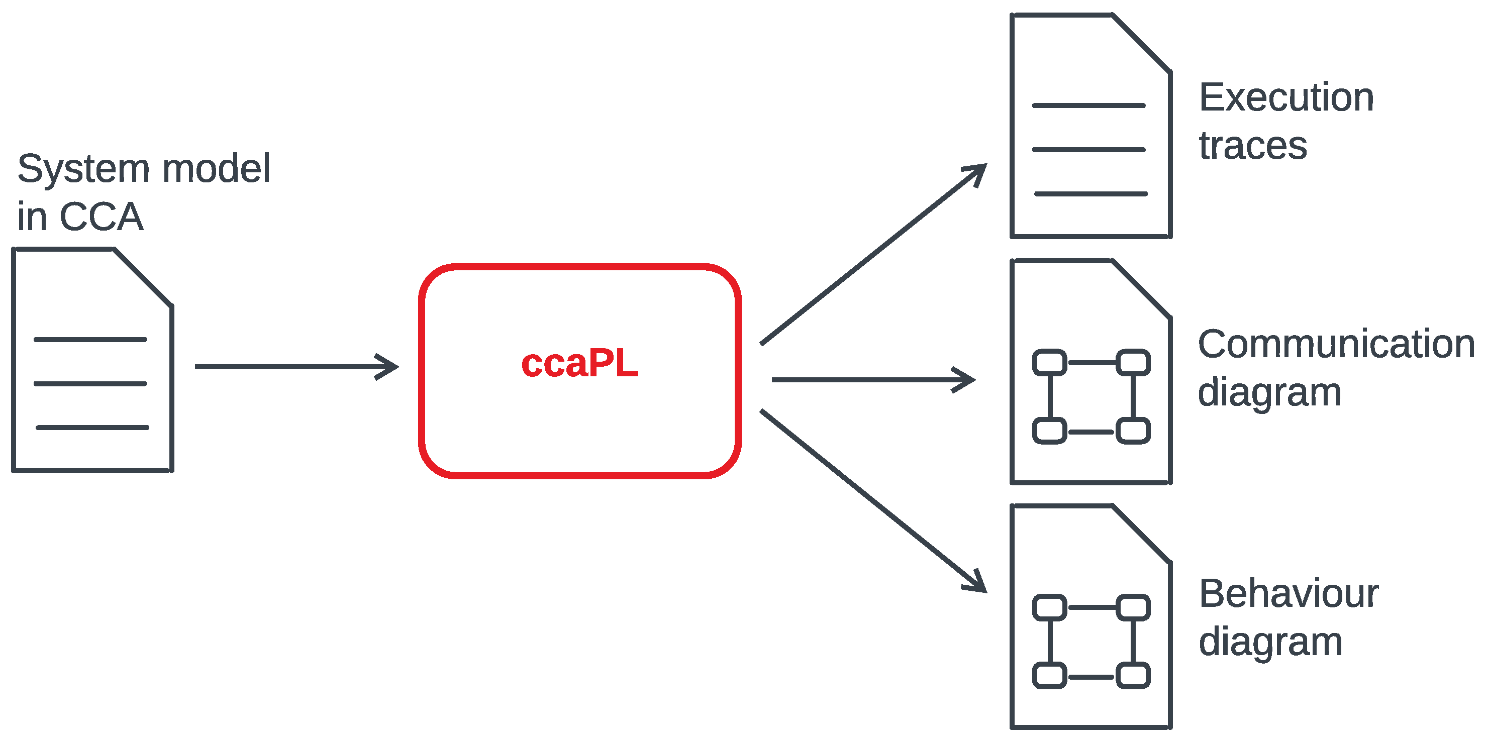
• An implementation of the algorithm in Python is provided (as a proof of concept) to automatically generate a CCA process that describes the behaviours of a given UML activity diagram (Appendix A). The experimental results confirm the theoretical complexity in time and in the output size of the algorithm with respect to the size of the input (Section 3.1). The generated process can be executed in various scenarios using the CCA simulation tool ccaPL to better understand the behaviours of the corresponding UML activity diagram.
• We extend the syntax and the semantics of the linear temporal logic (LTL) with the CCA notion of context expression and other new predicates to support the runtime verification of CCA processes (Section 3.3.1).
• A runtime verification tool, ccaRV, is implemented in Java and can be used to verify UML activity diagrams (Section 3.3). This tool checks at runtime whether a UML activity diagram satisfies a desired property specified as an LTL formula.
• The pragmatics of the proposed approach is demonstrated using a case study in e-commerce (Section 3.4).

The rest of the paper is structured as follows. Section 2 provides an overview of UML activity diagrams, CCA, and the algorithm for mapping a UML activity diagram onto a CCA process. Section 3 presents the experimental results, the simulation tool ccaPL, the runtime verification tool ccaRV, and a case study. Section 4 discusses the related work and the limitations of the proposed approach. Section 5 concludes the paper and points to future research directions.

2. Materials and Methods

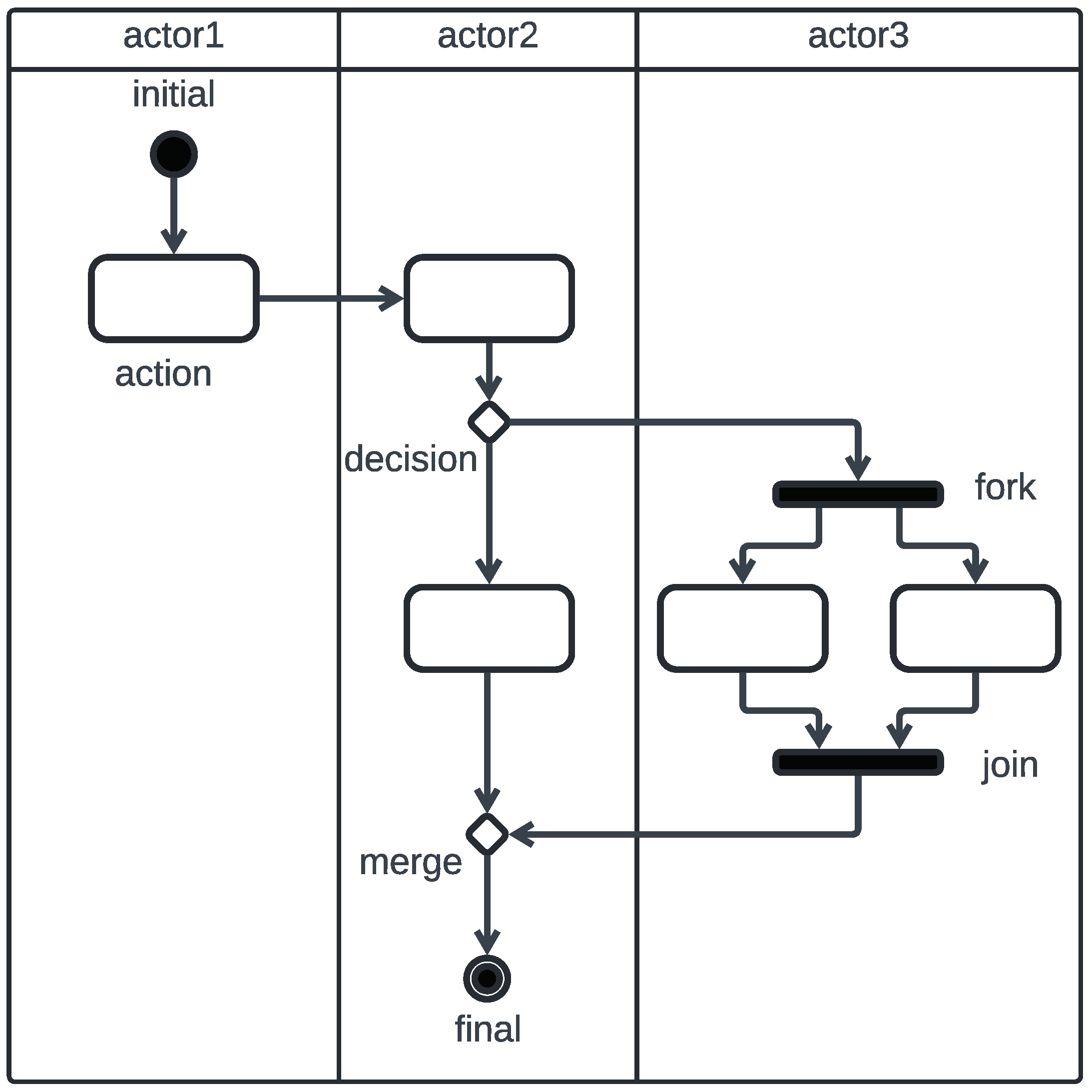
2.1. Overview of UML Activity Diagrams

A UML Activity diagram describes the behaviours of a system, represented as a flow of controls from activity to activity. An activity denotes a coordinated flow of actions that must be taken by the system [2]. For illustration, Figure 1 shows a typical UML activity diagram; the nodes of the diagram are called activity nodes, and the arcs between the nodes are called transitions. A transition indicates that the flow of control passes from one activity node to another activity node and is rendered as a directed line between the two activity nodes. There are different types of nodes. The flow of control of an activity diagram begins in the initial node, rendered as a solid ball, and terminates in a final node, rendered as a solid ball inside a circle. An action node represents a single atomic step within an activity and is rendered as a round-cornered rectangle. Special activity nodes called fork and join are used to synchronise parallel flows of control and are rendered as a thick horizontal line. A fork node has one incoming transition and two or more outgoing transitions, each of which represents an independent flow of control. A join node has two or more incoming transitions and one outgoing transition. It synchronises all the independent flows of control created by a fork node. Alternate flows based on Boolean expressions can be specified using a decision node rendered as a diamond. A decision node has one incoming transition and two or more outgoing transitions; each outgoing transition carries a Boolean expression, which must hold for that branch to be taken. These guards across outgoing transitions should not overlap and should cover all possibilities. A merge node is also rendered as a diamond and brings together multiple incoming alternate flows to accept a single outgoing flow. Unlike a join node, there is no synchronisation of alternate flows. Swimlanes are used to partition the activity nodes between the actors responsible for executing them. A swimlane boundary is rendered as a pair of parallel (vertical or horizontal) solid lines. There are other activity elements like object nodes and interrupting edges that are not included in the scope of this paper but can be handled in a similar manner.

Example 1.

Shopping order processing: The activity diagram shown in Figure 2 describes the step-by-step activities to be performed in the processing of a shopping order in an e-commerce application. This example is taken and adapted from the UML 2.4.1 Specification document [1]. In this activity diagram, there are two actors (swimlanes): a customer who requests an order and the order service that processes the order. The customer initiates the activity and sends an order request to the order service. If the request is accepted and all required information is filled in, an invoice is sent to the customer. In the meantime, the order is shipped while waiting for the customer to make the payment. The order is closed once the payment is accepted by the order service. Note that in this business model, an order can be shipped before the payment is received.

2.2. Overview of CCA

CCA [10,11] is a process calculus for specifying and reasoning about the behaviour of context-aware, mobile, and concurrent systems. CCA is based on a single notion of ambient, which conceptualises an entity in which a computation can occur. An ambient is represented in the form $n\left[P\right]$, where n is the name of the ambient and P is a process describing the behaviour of the ambient. We can also say that the process P is executed by the ambient n. An ambient can contain other ambients, called child ambients, forming a hierarchy of ambients. For example, in $n\left[P\right|m\left[Q\right]]$, n is the parent ambient of m, and m is a child ambient of n. Two ambients that have the same parent are siblings. There is a special ambient called root, which represents the root of the ambient hierarchy. Any ambient in CCA is a descendant of the root ambient. Ambients can be composed in parallel, using the parallel operator “|” to form a concurrent system. During their execution, ambients can communicate through a hand-shake message passing mechanism; i.e., an ambient (the sender) can send a message to another ambient (the receiver) and the sender and the receiver must synchronise for the communication to happen, as explained in Section 2.2.2. An ambient can be mobile; the mobility capabilities “$\mathtt{in}$” and “$\mathtt{out}$”, described in Section 2.2.2, allow an ambient to move inside a sibling ambient and outside its parent ambient, respectively. An ambient can also be aware of its context so that its behaviour can change in response to changes in the context. This is undertaken using context expressions and context-guarded processes (see Section 2.2.4). A context expression is a predicate over the state of the ambient hierarchy. In distributed systems, each component of a system can be modelled as an ambient, e.g., sensors and computers. An example is provided in Section 2.2.5.

CCA is formally described by the grammar in

Table 1. Syntax of CCA.

$\mathit{P},\mathit{Q}$	$::=$		Processes	$\kappa$	$::=$		Context Expressions
		$\mathtt{0}$	inactivity			$\mathtt{0}$	empty context
		$P|Q$	parallel composition			$\mathtt{true}$	true
		$\left\{P\right\}$	block			$\mathtt{false}$	false
		$\left(\mathtt{new}n\right)P$	name restriction			$n=m$	name match
		$!P$	replication			$\mathtt{this}$	hole
		$n\left[P\right]$	ambient			$n\left[\kappa \right]$	location context
		$<\kappa >M.P$	context-guarded prefix			${\kappa }_1|{\kappa }_2$	parallel composition
		$\mathtt{if}<{\kappa }_1>M_1.P_1$	if-then			${\kappa }_1\mathtt{and}{\kappa }_2$	conjunction
		…				${\kappa }_1\mathtt{or}{\kappa }_2$	disjunction
		$<{\kappa }_{\ell }>M_{\ell }.P_{\ell }\mathtt{fi}$				$\mathtt{not}\kappa$	negation
		$\mathtt{if}<{\kappa }_1>M_1.P_1$	if-then-else			$\mathtt{next}\kappa$	spatial next modality
		$\dots$				$\mathtt{somewhere}\kappa$	somewhere modality
		$<{\kappa }_{\ell }>M_{\ell }.P_{\ell }\mathtt{else}P\mathtt{fi}$
		$\mathtt{let}{x}_1=e_1,\dots ,x_{\ell }=e_{\ell }\mathtt{in}P$	arithmetic
		$\mathtt{find}{x}_1,\dots ,x_{\ell }:\kappa \mathtt{for}P$	search
		$\mathtt{proc}x(y_1,\dots ,y_{\ell })P$	process abstraction
M	$::=$		Capabilities	$\alpha$	$::=$		Locations
		$\mathtt{skip}$	one transition			@	any parent
		$\mathtt{in}n$	move into ambient n			$n@$	specific parent n
		$\mathtt{out}$	move out of parent			#	any child
		$\mathtt{del}n$	delete ambient n			$n\#$	specific child n
		$\alpha \mathtt{recv}(y_1,\dots ,y_{\ell })$	receive data from $\alpha$			$::$	any sibling
		$\alpha \mathtt{send}(z_1,\dots ,z_{\ell })$	send data to $\alpha$			$n::$	specific sibling n
		$\alpha x(z_1,\dots ,z_{\ell })$	process abstraction call			$ϵ$	locally

based on three syntactic categories: processes P (or Q), capabilities M, and context expressions $\kappa$. The symbols n, x, y, and z are names. Note that comments can be added anywhere in a specification using the prefix // for a single-line comment or the pair /* and */ for a multi-line comment.

2.2.1. Processes

The syntax of a process P is provided in Table 1. The process $\mathtt{0}$, also known as the inactivity process, does nothing and terminates immediately. The process $P|Q$ denotes the parallel composition of processes P and Q. A process of the form $\left\{P\right\}$ behaves just like P. The process $\left(\mathtt{new}n\right)P$ creates a new name n, and the scope of that name is limited to the process P. Replication $!P$ denotes a process which can always create a new parallel copy of P, i.e., $!P$ is equivalent to $P|!P$. The process $n\left[P\right]$ denotes an ambient named n whose behaviour is described by the process P. A context expression $\kappa$ is a logical formula that specifies a property upon the state of the environment. A context-guarded prefix $<\kappa >M.P$ is a process that waits until the environment satisfies the context expression $\kappa$, and then performs the capability M and continues like the process P. We let $M.P$ denote the process $<\mathtt{true}>M.P$. An if-then process $\mathtt{if}<{\kappa }_1>M_1.P_1\dots <{\kappa }_{\ell }>M_{\ell }.P_{\ell }\mathtt{fi}$ waits until at least one of the context expressions ${\left({\kappa }_i\right)}_{1\le i\le \ell }$ holds, and then proceeds non-deterministically like one of the $<{\kappa }_j>M_j.P_j$ processes for which ${\kappa }_j$ holds. An if-then-else process $\mathtt{if}<{\kappa }_1>M_1.P_1\dots <{\kappa }_{\ell }>M_{\ell }.P_{\ell }\mathtt{else}P\mathtt{fi}$ behaves like an if-then process but does not wait and continues like the P process if none of the branches can be executed. A process $\mathtt{let}{x}_1=e_1,\dots ,y_{\ell }=e_{\ell }\mathtt{in}P$ behaves like the process P in which each occurrence of $x_i$ is substituted to the value of the arithmetic expression $e_i$, for $1\le i\le \ell$ and $\ell \ge 1$. A search process $\mathtt{find}{x}_1,\dots ,x_{\ell }:\kappa \mathtt{for}P$ looks for a list of names $n_1,\dots ,n_{\ell }$ in the context such that the context expression $\kappa$ in which each occurrence of $x_i$ is replaced by $n_i$ holds, and continues like the process P in which each occurrence of $x_i$ is replaced with $n_i$, $1\le i\le \ell$ and $\ell \ge 1$. A process of the form $\mathtt{proc}x(y_1,\dots ,y_{\ell })P$, for some $\ell \ge 0$, defines a process abstraction named x, whose behaviour is described by the process P. The names $y_1,\dots ,y_{\ell }$ are the formal parameters of the process abstraction. A process abstraction is a mechanism to give a name, say x, to a process P and later use that name anywhere to refer to the process P, just the same way functions and procedures are used in programming languages.

2.2.2. Capabilities

A capability is an elementary action that an ambient can perform. The syntax of a capability M is provided in Table 1. The capability $\mathtt{skip}$ represents one transition, i.e., one execution step. An ambient can move into a sibling ambient n by performing the capability $\mathtt{in}n$ and move out of its parent ambient by executing the capability $\mathtt{out}$. An ambient can exchange messages with another ambient using the output capability $\alpha \mathtt{send}(z_1,\dots ,z_{\ell })$ to send a list of names $z_1,\dots ,z_{\ell }$ to a location $\alpha$ and the input capability $\alpha \mathtt{recv}(y_1,\dots ,y_{\ell })$ to receive a list of names from a location $\alpha$ in the variables $y_1,\dots ,y_{\ell }$ for some $\ell \ge 0$. The location $\alpha$ can be @ to mean any parent, $n@$ to mean a specific parent n, # to mean any child ambient, $n\#$ to mean a specific child n, $::$ to mean any sibling, $n::$ to mean a specific sibling n, or  $ϵ$ (empty string) to mean the executing ambient itself. A capability $\mathtt{del}n$ deletes an empty child ambient n (i.e., $n\left[\mathtt{0}\right]$). A capability of the form $\alpha x(z_1,\dots ,z_{\ell })$ calls the process abstraction x defined at the location $\alpha$, and the names $z_1,\dots ,z_{\ell }$ are the actual parameters, $\ell \ge 0$.

2.2.3. Context Model

In CCA, a context is modelled as a process with possibly a single hole in it. The hole (denoted by ⊙) in a context C represents the position of the process, for which C is a context. For example, suppose a system is modelled by the process $P\left|n\right[Q\left|m\right[R\left|S\right]]$. Therefore, the context of the process R in that system is $P\left|n\right[Q\left|m\right[\odot \left|S\right]]$, and  that of the ambient named m is $P\left|n\right[Q|\odot ]$. Thus, the context of a CCA process is described by the grammar in

Table 2. Syntax of contexts.

C

$::=$

$P|\odot |n\left[C\right]\left|C\right|P\left|\right(\mathtt{new}n\left)C\right|\left\{C\right\}$

and satisfies the following congruence rules: $\mathtt{0}|C\equiv C$, $\left\{C\right\}\equiv C$, and $C|P\equiv P|C$. A context expression (CE, for short) is a formula representing a property over context.

2.2.4. Context Expressions

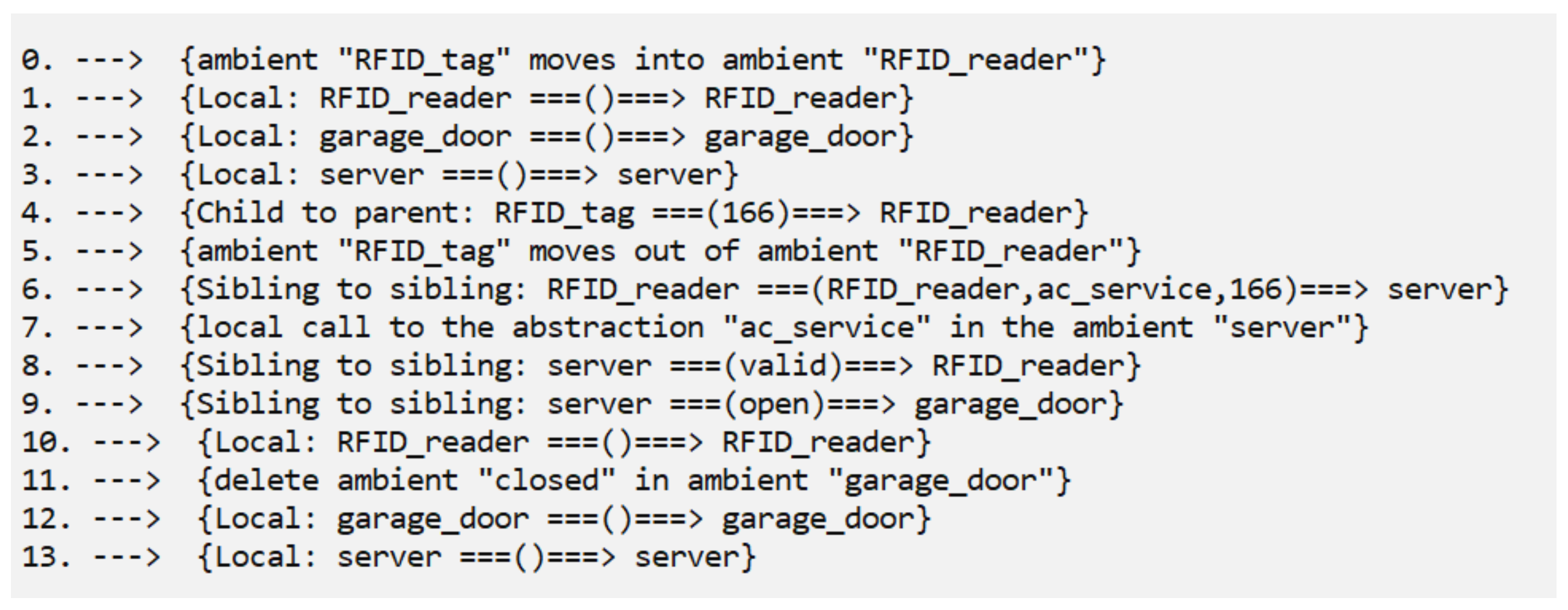
The syntax of a process expression $\kappa$ is provided in Table 1. The formal semantics of context expressions (CEs) with respect to the context model of Table 2 are presented in

Table 3. Satisfaction relation for context expressions.

	⊧	$\mathtt{true}$
C	⊧	$n=m$	if	$n=m$
C	⊧	$\mathtt{0}$	if	$C=\mathtt{0}$
C	⊧	$\mathtt{this}$	if	$C=\odot$
C	⊧	$\mathtt{not}\kappa$	if	Cκ
C	⊧	${\kappa }_1|{\kappa }_2$	if	$\mathrm{exist}{C}_1,C_2\mathrm{such}\mathrm{that}C=C_1|C_2$$\mathrm{and}{C}_1\vDash {\kappa }_1\mathrm{and}{C}_2\vDash {\kappa }_2$
C	⊧	${\kappa }_1\mathtt{and}{\kappa }_2$	if	$C\vDash {\kappa }_1\mathrm{and}C\vDash {\kappa }_2$
C	⊧	$n\left[\kappa \right]$	if	$\mathrm{exists}{C}^{\prime }\mathrm{such}\mathrm{that}C=n\left[C^{\prime }\right]\mathrm{and}{C}^{\prime }\vDash \kappa$
C	⊧	$\mathtt{next}\kappa$	if	$\mathrm{exist}{C}^{\prime },n\mathrm{such}\mathrm{that}C=n\left[C^{\prime }\right]\mathrm{and}{C}^{\prime }\vDash \kappa$
C	⊧	$\mathtt{somewhere}\kappa$	if	$C\vDash \kappa$ or $\mathrm{exist}{C}^{\prime },n\mathrm{such}\mathrm{that}C=n\left[C^{\prime }\right]\mathrm{and}$ $C^{\prime }\vDash \mathtt{somewhere}\kappa$

, where the notation $C\vDash \kappa$ means that the context C satisfies the context expression $\kappa$. We also write $\vDash \kappa$ to mean that a context expression $\kappa$ is valid, i.e., $\kappa$ is satisfied by all contexts.

The CE $\mathtt{true}$ holds for all contexts, while the CE $\mathtt{false}$ holds for no context. A CE $n=m$ holds if the names n and m are identical. The CE $\mathtt{0}$ holds for the empty context $\mathtt{0}$. The CE $\mathtt{this}$ holds solely for the whole context, i.e., the position of the process evaluating that context expression. Propositional operators such as $\mathtt{not}$, $\mathtt{and}$, and $\mathtt{or}$ expand their usual semantics to context expressions. A CE ${\kappa }_1|{\kappa }_2$ holds for a context if that context is a parallel composition of two contexts such that ${\kappa }_1$ holds for one and ${\kappa }_2$ holds for the other. A CE $n\left[\kappa \right]$ holds for a context if that context is an ambient named n such that $\kappa$ holds inside that ambient. A CE $\mathtt{next}\kappa$ holds for a context if that context has a child context for which $\kappa$ holds. A CE $\mathtt{somewhere}\kappa$ holds for a context if there exists somewhere in that context a sub-context for which $\kappa$ holds. Some examples of context expressions are provided in

Table 4. Examples of context expressions.

$has\left(n\right)$	=	$\mathtt{somewhere}\left(\mathtt{this}\right|n\left[\mathtt{true}\right]\left|\mathtt{true}\right)$	n is located at self.
$at\left(n\right)$	=	$\mathtt{somewhere}\left(n\right[\mathtt{next}\left(\mathtt{this}\right|\mathtt{true}\left)\right]\left|\mathtt{true}\right)$	self is located at n.
$at(n,m)$	=	$\mathtt{somewhere}\left(n\right[m\left[\mathtt{true}\right]\left|\mathtt{true}\right]\left|\mathtt{true}\right)$	m is located at n.
$with\left(n\right)$	=	$\mathtt{somewhere}\left(n\right[\mathtt{true}\left]\right|\mathtt{next}\left(\mathtt{this}\right|\mathtt{true}\left)\right|\mathtt{true})$	self is with n.
$with(n,m)$	=	$\mathtt{somewhere}\left(n\right[\mathtt{true}\left]\right|m\left[\mathtt{true}\right]\left|\mathtt{true}\right)$	n is with m.
$state\left(n\right)$	=	$\mathtt{somewhere}\left(\mathtt{this}\right|n\left[0\right]\left|\mathtt{true}\right)$	current state of self is n.
$state(d,n)$	=	$\mathtt{somewhere}\left(d\right[n\left[0\right]\left|\mathtt{true}\right]\left|\mathtt{true}\right)$	current state of a device d is n.
$notEnd\left(\right)$	=	$\mathtt{somewhere}\left(final\right[0\left]\right|\mathtt{true})$	there exists an ambient of the
			form $final$[0].

.

Context expressions are used in CCA to specify context-aware processes. We recall in

Table 5. Semantics of context-aware processes.

(R1)	$C(M.P)⟶C^{\prime }\left(P\sigma \right)\Rightarrow C(<\kappa >M.P)⟶C^{\prime }\left(P\sigma \right)$   if $C\vDash \kappa$
(R2)	$C(<{\kappa }_i>M_i.P_i)⟶C^{\prime }\left(P_i\sigma \right)$
	$\Rightarrow C(\mathtt{if}<{\kappa }_1>M_1.P_1\dots <{\kappa }_{\ell }>M_{\ell }.P_{\ell }\mathtt{fi})⟶C^{\prime }\left(P_i\sigma \right)$, for some i, $1\le i\le \ell$.
(R3)	$C(\mathtt{if}<{\kappa }_1>M_1.P_1\dots <{\kappa }_{\ell }>M_{\ell }.P_{\ell }\mathtt{fi})⟶C^{\prime }\left(P_i\sigma \right)$
	$\Rightarrow C(\mathtt{if}<{\kappa }_1>M_1.P_1\dots <{\kappa }_{\ell }>M_{\ell }.P_{\ell }\mathtt{else}P\mathtt{fi})⟶C^{\prime }\left(P_i\sigma \right)$
(R4)	$C(\mathtt{if}<{\kappa }_1>M_1.P_1\dots <{\kappa }_{\ell }>M_{\ell }.P_{\ell }\mathtt{else}P\mathtt{fi})⟶C\left(P\right)$
	if $\forall i\in [1,\ell ]$ $(C^{\prime },\sigma )\mathrm{such}\mathrm{that}C(<{\kappa }_i>M_i.P_i)⟶C^{\prime }\left(P_i\sigma \right)$.
(R5)	$C(\mathtt{find}{x}_1,\dots ,x_{\ell }:\kappa \mathtt{for}P)⟶C\left(P\{x_1\leftarrow n_1,\dots ,x_{\ell }\leftarrow n_{\ell }\}\right)$
	if $C\vDash \kappa \{x_1\leftarrow n_1,\dots ,x_{\ell }\leftarrow n_{\ell }\}$
(R6)	$C(\mathtt{let}{x}_1=e_1,\dots ,x_{\ell }=e_{\ell }\mathtt{in}P)\equiv C\left(P\{x_1\leftarrow val\left(e_1\right),\dots ,x_{\ell }\leftarrow val\left(e_{\ell }\right)\}\right)$
(R7)	$\mathtt{skip}.P⟶P$
(R8)	$\mathtt{del}n.P\left|n\right[\mathtt{0}]⟶P$
(R9)	$!P\equiv P|!P$
(R10)	$\mathtt{recv}(y_1,\dots ,y_{\ell }).P|\mathtt{send}(z_1,\dots ,z_{\ell }).Q⟶P\{y_1\leftarrow z_1,\dots ,y_{\ell }\leftarrow z_{\ell }\}|Q$, for $\ell \ge 0$
(R11)	$n[::\mathtt{recv}(y_1,\dots ,y_{\ell }).P|R]|m[::\mathtt{send}(z_1,\dots ,z_{\ell }).Q|S]⟶$
	$n\left[P\{y_1\leftarrow z_1,\dots ,y_{\ell }\leftarrow z_{\ell }\}\right|R]|m\left[Q\right|S]$, for $\ell \ge 0$
(R12)	$n[::\mathtt{recv}(y_1,\dots ,y_{\ell }).P|R]|m[n::\mathtt{send}(z_1,\dots ,z_{\ell }).Q|S]⟶$
	$n\left[P\{y_1\leftarrow z_1,\dots ,y_{\ell }\leftarrow z_{\ell }\}\right|R]|m\left[Q\right|S]$, for $\ell \ge 0$
(R13)	$n[m::\mathtt{recv}(y_1,\dots ,y_{\ell }).P|R]|m[::\mathtt{send}(z_1,\dots ,z_{\ell }).Q|S]⟶$
	$n\left[P\{y_1\leftarrow z_1,\dots ,y_{\ell }\leftarrow z_{\ell }\}\right|R]|m\left[Q\right|S]$, for $\ell \ge 0$
(R14)	$n[m::\mathtt{recv}(y_1,\dots ,y_{\ell }).P|R]|m[n::\mathtt{send}(z_1,\dots ,z_{\ell }).Q|S]⟶$
	$n\left[P\{y_1\leftarrow z_1,\dots ,y_{\ell }\leftarrow z_{\ell }\}\right|R]|m\left[Q\right|S]$, for $\ell \ge 0$

the formal semantics of context-aware processes, where $\sigma$ is a substitution of names, ≡ is the congruence relation of processes, and ⟶ is the reduction relation of processes. The notation $val\left(e\right)$ represents the value of an expression e. The complete formal semantics of CCA can be found in [10,11].

2.2.5. An Example

This example illustrates how to model a distributed system in CCA. Consider a simple access control system that is composed of an RFID reader, an RFID tag, a server, and a garage door. Only authorised users can access the garage through the door. When an RFID tag is detected by the RFID reader, the ID (also known as identification) number of the tag is transmitted to the reader, which then sends an access request to the server. The server checks if the ID number is permitted to access the garage (i.e., valid), in which case the garage door opens. If the ID number is not permitted to be accessed (i.e., invalid), the door stays closed. Let us assume that a valid ID number is exclusively a value between 100 and 200. Each component (RFID tag, RFID reader, garage door, and server) of this distributed system can be modelled as an ambient in CCA.

Indeed, an RFID tag is a device that stores an ID number. The ID number is sent to an RFID reader when the tag is in the range of the reader. In CCA, an RFID tag and an RFID reader can be represented as ambients. The boundary of the reader ambient delimits the range of the reader, i.e., an RFID tag is in the range of a reader if that tag is a child ambient of the reader. An RFID tag that contains the ID number 166 can be modelled in CCA according to the ambient in Listing 1. It is assumed that initially, the RFID tag is not in the range of the RFID reader, but then it moves into the range of the reader using the capability “in” (described in Section 2.2). After the ID number is read, the RFID tag moves away from the reader using the capability “out”.

Listing 1. The ambient representing the RFID tag.

RFID_tag[      !@send(166).out.0    | in RFID_reader.0 ]

An RFID reader can be specified, as in Listing 2. It reads the value of an RFID tag and requests the access control service (ac_service) from the server. Upon receipt of a response (status) from the server, the reader shows a green light (status=valid) to indicate that the access request is authorised or a red light (status=invalid) if the access request is denied.

Listing 2. The ambient representing the RFID reader.

RFID_reader[      !recv().#recv(id).server::send(RFID_reader, ac_service, id).          server::recv(status).send().0    | send().0 ]

The server can be modelled as the ambient in Listing 3. It receives a service request from a client and executes the requested service. A service is modelled as a process abstraction. In this example, there is only one service: the access control service ac_service.

Listing 3. The ambient representing the server.

server[      proc ac_service(client, door, id) {         if            < (id>100) and (id<200) > client::send(valid).                  door::send(open).send().0         else           client::send(invalid).door::send(close).send().0         fi      }    |      !recv().::recv(client, service, id).service(client, garage_door, id).0    | send().0 ]

The last component of the system to specify is the garage door. The door can be controlled by the server and is modelled by the ambient in Listing 4. It closes if it receives the command “close” from the server and opens if it receives the command “open”. The current state of the door (closed/opened) is checked using the context expression $state\left(n\right)$ defined in Table 4.

The overall access control system is modelled in Listing 5 as the parallel composition of its four components described in Listings 1–4. The declaration block, which starts with the keyword BEGIN_DECLS and ends with the keyword END_DECLS, contains the definition of the context expression $state\left(n\right)$ and other execution directives explained in Section 3.2.

Listing 4. The ambient representing the garage door.

garage_door[      !recv().server::recv(x).         if            < x = close and state(opened) > del opened.send().closed[0]            < x = open and state(closed) > del closed.send().opened[0]         else            send().0         fi    | send().0    | closed[0] // initially the door is closed. ]

Listing 5. The CCA process representing the access control system of Section 2.2.5.

BEGIN_DECLS    def state(n) = { somewhere (this | n[0] | true) }    //display code    //display congruence    mode random    //length = 100 END_DECLS RFID_tag[      !@send(166).out.0    | in RFID_reader.0 ] | RFID_reader[      !recv().#recv(id).server::send(RFID_reader, ac_service, id).          server::recv(status).send().0    | send().0 ] | server[      proc ac_service(client, door, id) {         if            < (id>100) and (id<200) > client::send(valid).                  door::send(open).send().0         else           client::send(invalid).door::send(close).send().0         fi      }    |      !recv().::recv(client, service, id).service(client, garage_door, id).0    | send().0 ] | garage_door[      !recv().server::recv(x).         if            < x = close and state(opened) > del opened.send().closed[0]            < x = open and state(closed) > del closed.send().opened[0]         else            send().0         fi    | send().0    | closed[0] // initially the door is closed. ]

Since CCA specifications are executable, the simple access control system can be analysed using the CCA simulator ccaPL, and the simulation outputs are illustrated in Section 3.2. Moreover, an example of how the simple access control system can be verified using the CCA runtime verification tool ccaRV is provided in Section 3.3.2. The next section presents an algorithm for mapping a UML activity diagram onto a CCA process.

2.3. Mapping an Activity Diagram onto a CCA Process

This section presents an algorithm for mapping a UML activity diagram onto a CCA process. Given a UML activity diagram represented in the tuple structure described in Section 2.3.1, the algorithm generates a CCA process that models the behaviour of the activity diagram.

Table 6. Mapping of the UML activity diagram concepts onto the CCA concepts.

UML Concepts	CCA Concepts
activity node	process abstraction
transition	process abstraction call
actor (or swimlane)	ambient

shows how the concepts of a UML activity diagram (Section 2.1) are mapped to the concepts of CCA (Section 2.2).

2.3.1. A Mathematical Representation of an Activity Diagram

An activity diagram can be represented by the tuple $(N,T,A,C,mN,mT,mA,mC)$, where

• N is a non-empty finite set of activity nodes. It is assumed that no two activity nodes have the same name.
• $T\subseteq \left\{\right(x,y\left)\right|x,y\in N\mathrm{and}x\ne y\}$ is a set of transitions.
• A is a finite set of actors (i.e., swimlanes).
• C is a finite set of the conditions (i.e., Boolean expressions) carried by decision nodes.
• $mT\subseteq \left\{\right(x,y\left)\right|x\in N\mathrm{and}y\in \{initial,action,fork,join,decision,merge,final\}\}$ is a type assignment to activity nodes.
• $mN\subseteq \left\{\right(x,y\left)\right|x,y\in N\mathrm{and}mT\left(x\right)=fork\mathrm{and}mT\left(y\right)=join\}$ is a mapping of fork nodes to the corresponding join nodes.
• $mA\subseteq N\times A$ is a mapping of activity nodes to the actors that perform them.
• $mC\subseteq \left\{\right(x,y,z\left)\right|(x,y,z)\in C\times N\times N\mathrm{and}mT\left(y\right)=decision\mathrm{and}(y,z)\in T\}$ is a mapping of conditions to the decision node branches.

Example 2.

The activity diagram in Figure 2 is represented by the tuple $(N,T,A,C,mN,mT,mA,mC)$, where

• $N=\{initial,Request\_Order,Receive\_Order,decision,Fill\_Order,fork,Ship\_Order,$
  $Send\_Invoice,Make\_Payment,Accept\_Payment,join,merge,Close\_Order,final\}$.
• $T=\left\{\right(initial,Request\_Order),(Request\_Order,Receive\_Order),$
  $(Receive\_Order,decision),(decision,Fill\_Order),(Fill\_Order,fork),$
  $(fork,Ship\_Order),(fork,Send\_Order),(Send\_Invoice,Make\_Payment),$
  $(Make\_Payment,Accept\_Payment),(Accept\_Payment,join),(Ship\_Order,join),$
  $(join,merge),(decision,merge),(merge,Close\_Order),(Close\_Order,final)\}$.
• $A=\{Customer,Order\_Service\}$.
• $C=\{accept,reject\}$.
• $mT=\left\{\right(initial,initial),(Request\_Order,action),(Receive\_Order,action),$
  $(decision,decision),(Fill\_Order,action),(fork,fork),(Send\_Invoice,action),$
  $(Make\_Payment,action),(Accept\_Payment,action),(Ship\_Order,action),$
  $(join,join),(merge,merge),(Close\_Order,action),(final,final)\}$.
• $mN=\left\{\right(fork,join\left)\right\}$.
• $mA=\left\{\right(initial,Customer),(Request\_Order,Customer),(decision,Order\_Service),$
  $(Receive\_Order,Order\_Service),(Fill\_Order,Order\_Service),(fork,Order\_Service),$
  $(Ship\_Order,Order\_Service),(Send\_Invoice,Order\_Service),(final,Order\_Service),$
  $(Accept\_Payment,Order\_Service),(join,Order\_Service),(merge,Order\_Service),$
  $(Make\_Payment,Customer),(Close\_Order,Order\_Service)\}$.
• $mC=\left\{\right(accept,decision,Fill\_Order),(reject,decision,merge\left)\right\}$.

This representation of an activity diagram is used in the following section to devise an algorithm for translating an activity diagram into a CCA process.

2.3.2. An Algorithm for Mapping an Activity Diagram onto a CCA Process

The proposed algorithm takes as input an activity diagram represented like in Section 2.3.1 and generates a CCA process. This algorithm is provided in Algorithm 1, which calls on Algorithm 2 to process each activity node. The output of Algorithm 1 is calculated as a string in the variable $cca\_str$. In line 1, the variables $SPACE$ and $SPACE1$ are each set to a string of three space characters and are used merely for code indentations. In line 2, a declaration block is created starting with the keyword BEGIN_DECLS and containing the definitions of the context expressions $state\left(n\right)$ and $notEnd\left(\right)$ provided in Table 4. The context expression $state\left(n\right)$ holds if the ambient executing it has a child ambient of the form $n\left[0\right]$. The context expression $notEnd\left(\right)$ holds if the execution has not yet reached the final node of the activity diagram. Lines 3–4 create for each decision node y a context expression definition of the form def y(n) = { n = c }, where c is one of the conditions carried by the decision node y. In line 5, the execution directives display code, display congruence, mode random, and length are added into the declaration block, which is then closed with the keyword END_DECLS. For example, the execution directive length = 100 causes the execution to stop after a maximum of 100 execution steps. More details about the structure and content of a declaration block are provided in Section 3.2. In summary, the general form of the declaration block generated in lines 2–5 of Algorithm 1 is presented in Listing 6. Moreover, Example 3 shows the declaration block generated by Algorithm 1 for the activity diagram of Figure 2.

Example 3.

The declaration block generated by Algorithm 1 for the activity diagram of Figure 2 is the following.

BEGIN_DECLS

   def state(n) = { somewhere (this | n[0] | true) }

   def notEnd() = { somewhere (final[0] | true) }

   def decision(n) = { n = accept }

   //display code

   //display congruence

   mode random

   //length = 100

END_DECLS

Listing 6. General form of a declaration block generated by Algorithm 1.

BEGIN_DECLS    def state(n) = { somewhere (this | n[0] | true) }    def notEnd() = { somewhere (final[0] | true) }    def decision1(n) = { n = c1 }    …    def decisionN(n) = { n = cN }    //display code    //display congruence    mode random    //length = 100 END_DECLS

Algorithm 1: Mapping a UML activity diagram onto a CCA process.

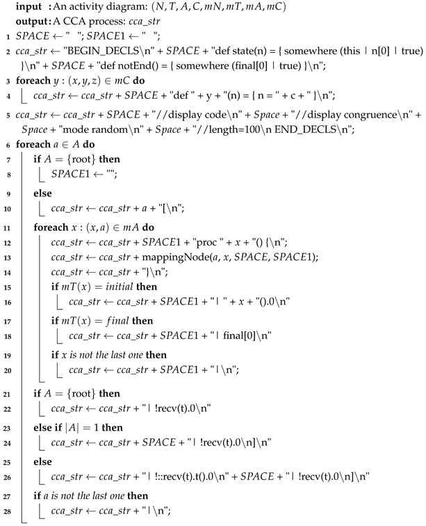
Algorithm 2: mappingNode(a, x, SPACE, SPACE1).

The loop in lines 6–28 creates for each actor/swimlane $a\in A$ an ambient of the same name (lines 7–24) and composes in parallel (lines 27–28) all the ambients created. The loop in lines 11–20 creates for each node x in swimlane a a process abstraction of the same name x (line 12). The body of the process abstraction is calculated by Algorithm 2 (line 13) according to the type of the node x. The general forms of the process abstractions generated for each type of node are provided in

Table 7. Mapping of an initial, a final, and an action node onto a process abstraction. Columns A and B are swimlanes, and circles represent the next node.

Activity Diagram Node	Corresponding CCA Process
	proc initial() {   if     < notEnd() > send(initial).node().0   else skip.0   fi.0 }
	proc initial() {   if     < notEnd() > send(initial).       B::send(node).0   else skip.0   fi.0 }
	proc final() {   del final.send(final).0 }
	proc action() {   if     < notEnd() > send(action).node().0   else skip.0   fi.0 }
	proc action() {   if     < notEnd() > send(action).       B::send(node).0   else skip.0   fi.0 }

,

Table 8. Mapping of a decision node and a merge node onto a process abstraction. Columns A and B are swimlanes, and circles represent the next node.

Activity Diagram Node	Corresponding CCA Process
	proc decision() {   if     < notEnd() > send(decision).if       < decision(c1) > node1().0       …       < decision(c(N-1)) > node(N-1)().0     else nodeN().0     fi.0   else skip.0   fi.0 }
	proc decision() {   if     < notEnd() > send(decision).if       < decision(c1) > node1().0       …     else B::send(nodeN).0     fi.0   else skip.0   fi.0 }
	proc merge() {   if     < notEnd() > send(merge).node().0   else skip.0   fi.0 }
	proc merge() {   if     < notEnd() > send(merge).       B::send(node).0   else skip.0   fi.0 }

and

Table 9. Mapping of a fork node and a join node onto a process abstraction. Columns A and B are swimlanes, and circles represent the next node.

Activity Diagram Node	Corresponding CCA Process
	proc fork() {   if     < notEnd() > send(fork).{       node1() | join[0]       …      | nodeN().0 | join[0]     }   else skip.0   fi.0 }
	proc fork() {   if     < notEnd() > send(fork).{       node1() | join[0]       …      | B::send(nodeN).0 | join[0]     }   else skip.0   fi.0 }
	proc join() {   if     < notEnd() > del join.if       < state(join) > skip.0     else send(join).node().0     fi.0   else skip.0   fi.0 }
	proc join() {   if     < notEnd() > del join.if       < state(join) > skip.0     else send(join).B::send(node).0     fi.0   else skip.0   fi.0 }

. However, if node x is the initial node, then a call to the process abstraction x is added to the body of the ambient corresponding to the swimlane a (lines 15–16). Likewise, if the node x is the final node, then a child ambient final[0] is added to the body of the ambient corresponding to the swimlane a (lines 17–18). If there is more than one swimlane, then the process !::recv(t).t().0 is added to the body of the ambient corresponding to the swimlane a (lines 25–26). This process is used to handle the flows of control coming from a different actor/swimlane. In any case, the process !recv().0 is added to the body of the ambient a (lines 22, 24, and 26). This process is used to handle the local flows of control within a swimlane. In summary, the general forms of an ambient representing a swimlane (or an actor) are provided in Listings 7–10 depending on whether or not the swimlane a contains an initial node and/or a final node. Moreover, Example 4 shows the ambient generated by Algorithm 1 for the swimlane/actor “Customer” of the activity diagram of Figure 2.

Example 4.

The ambient generated by Algorithm 1 for the swimlane/actor “Customer” of the activity diagram of Figure 2 is specified as follows.

Customer[

   proc initial() {

      if

         < notEnd() > send(initial).Request_order().0

      else skip.0

      fi.0

   }

   | initial().0

   |

   proc Request_order() {

      if

         < notEnd() > send(Request_order).

            Order_service::send(Recv_order).0

      else skip.0

      fi.0

   }

   |

   proc Make_payment() {

      if

         < notEnd() > send(Make_payment).

            Order_service::send(Accept_payment).0

      else skip.0

      fi.0

   }

   | !::recv(t).t().0

   | !recv(t).0

]

Listing 7. General form of an ambient corresponding to a swimlane/actor that contains no initial node and no final node. The process abstractions node1(), …, nodeN() correspond to the activity nodes that belong to that swimlane.

a[    proc nod1(){       …    }    |    …    |    proc nodN(){       …    }    | !::recv(t).t().0    | !recv(t).0 ]

Listing 8. General form of an ambient corresponding to a swimlane/actor that contains an initial node and no final node. The process abstractions node1(), …, nodeN() correspond to the activity nodes that belong to that swimlane.

a[    proc initial(){       …    }    | initial().0    |    proc nod1(){       …    }    |    …    |    proc nodN(){       …    }    | !::recv(t).t().0    | !recv(t).0 ]

Listing 9. General form of an ambient corresponding to a swimlane/actor that contains no initial node but a final node. The process abstractions node1(), …, nodeN() correspond to the activity nodes that belong to that swimlane.

a[    proc final(){       …    }    |    proc nod1(){       …    }    |    …    |    proc nodN(){       …    }    | final[0]    | !::recv(t).t().0    | !recv(t).0 ]

Listing 10. General form of an ambient corresponding to a swimlane/actor that contains an initial node and a final node. The process abstractions node1(), …, nodeN() correspond to the activity nodes that belong to that swimlane.

a[    proc initial(){       …    }    | initial().0    |    proc final(){       …    }    |    proc nod1(){       …    }    |    …    |    proc nodN(){       …    }    | final[0]    | !::recv(t).t().0    | !recv(t).0 ]

Algorithm 2 calculates the body of the process abstraction corresponding to an activity node based on the type of the activity node. The algorithm takes four arguments: a swimlane a, an activity node x in the swimlane a, and two strings $SPACE$ and $SPACE1$ used for code indentations. The output of Algorithm 2 is calculated in the string variable $RES$. In line 1, $RES$ is initialised to an empty string. In lines 2–9, the body of the process abstraction for an initial node or an action node is created in $RES$. The result is illustrated in Table 7, depending on whether the successor node belongs to the same swimlane or not. It is assumed that only the final node does not have a successor node. The behaviour of the process abstraction generated in Table 7 can be explained as follows.

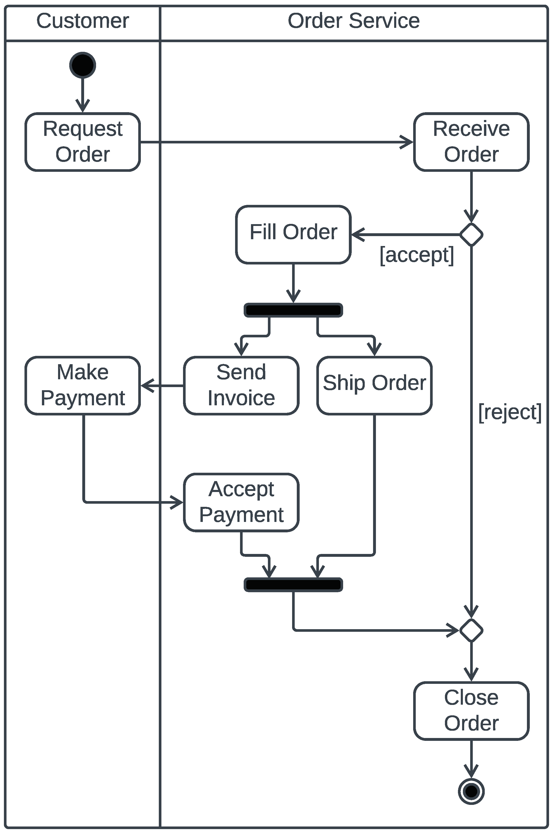
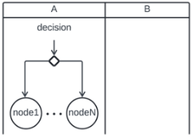
• When the successor node is in the same swimlane, the process abstraction checks if the final node is not reached yet (using the context expression notEnd()), in which case it executes the current activity node (by sending out the name of the node, e.g., send(initial)) and then transfers the control to the successor node (by calling the process abstraction corresponding to the successor node, i.e.,  node().0). Otherwise it terminates. Recall that each ambient corresponding to a swimlane contains the process !recv(t).0. This process is used to handle all the $send\left(x\right)$ statements corresponding to the execution of a local node x. For example, the process abstraction generated for the initial node of the activity diagram in Figure 2 is provided in Example 4.
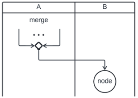
• When the successor node is in a different swimlane B, the process abstraction checks if the final node is not reached yet (using the context expression notEnd()), in which case it executes the current activity node (by sending out the name of the node, e.g., send(initial)) and then transfers the control to the successor node in the swimlane B (by sending the successor node name to B, i.e.,  B::send(node).0). Otherwise it terminates. Upon the receipt of the successor node name by B, the ambient B (representing the swimlane B) calls the process abstraction corresponding to that successor node using the process !::recv(t).t().0. Recall that when there are more than one swimlanes, each ambient corresponding to a swimlane contains the process !::recv(t).t().0, exactly for this purpose. For example, the process abstraction generated for the action node “Request Order” of the activity diagram in Figure 2 is provided in Example 4.

In lines 10–21 of Algorithm 2, the process abstraction corresponding to a decision node is created. It follows that each branch of a decision node is guarded using the context expression defined in the declaration block for that decision node. Recall that for each decision node x, a context expression of the same name $x\left(n\right)$ is defined in the declaration block, like in Listing 6. In lines 12–20, each branch of a decision node with condition c is represented by a branch in a CCA if-statement guarded by the context expression $x\left(c\right)$. The general form of a process abstraction generated for a decision node is given in Table 8. The behaviour of the process abstraction can be explained as follows. First, the process abstraction checks that the final node is not yet reached (using the context expression notEnd()); otherwise, it terminates immediately. If the final node has not yet been reached, then the branch that the guard holds is executed; there must be exactly one such branch as required by the UML standard. A branch $(c,x,z)\in mC$ (where c is the condition of the branch, x is the decision node, and z is the successor of x in that branch) is represented by a process of the form “$<x\left(c\right)>z\left(\right).0$” if x and z are in the same swimlane (like in Example 5), or of the form “$<x\left(c\right)>B::send\left(z\right).0$” if z belongs to a different swimlane B.

Example 5.

The process abstraction generated by Algorithm 1 for the decision node in the activity diagram of Figure 2 is as follows.

proc decision() {

   if

      < notEnd() > send(decision).if

            < decision(accept) > Fill_order().0

         else merge().0

         fi.0

   else skip.0

   fi.0

}

Lines 22–31 of Algorithm 2 generate a process abstraction for a fork node. The general form of the process abstraction generated is presented in Table 9. The loop in lines 24–30 creates for each successor node z of a fork node x a parallel process of the form “$z\left(\right).0\left|y\right[0]$” if x and z belong to the same swimlane (like in Example 6), or of the form “$B::send\left(z\right).0\left|y\right[0]$” if z belongs to a different swimlane B, where $y=mN\left(x\right)$ is the join node corresponding to the fork node x. The ambient $y\left[0\right]$ is used for synchronisation at the join node y so that the join node is executed only after all the independent flows of control of the fork node x have terminated.

Example 6.

The process abstraction generated by Algorithm 1 for the fork node in the activity diagram of Figure 2 is as follows.

proc fork() {

   if

      < notEnd() > send(fork).{

            Send_invoice().0 | join[0]

            | Ship_order().0 | join[0]

         }

   else skip.0

   fi.0

}

A process abstraction for a merge node is created in lines 32–37 of Algorithm 2. The general form of the process abstraction created is provided in Table 8. This process abstraction behaves as follows. If the context expression notEnd() does not hold (i.e., the final node of the activity diagram has been executed), then the process abstraction terminates immediately. Otherwise the merge node is executed (i.e., send(merge)) and then control is transferred to the successor node by calling the process abstraction corresponding to the successor node (i.e., node().0) if both belong to the same swimlane or, if not by sending the name of the successor node to the swimlane B it belongs to (i.e., B::send(node).0). For example, the process abstraction generated by Algorithm 1 for the merge node in the activity diagram of Figure 2 is provided in Example 7.

Example 7.

The process abstraction generated by Algorithm 1 for the merge node in the activity diagram of Figure 2 is the following.

proc merge() {

   if

      < notEnd() > send(merge).Close_order().0

   else skip.0

   fi.0

}

In lines 38–44 of Algorithm 2, a process abstraction for a join node is created. The general form of the process abstraction generated is provided in Table 9. The behaviour of the process abstraction is as follows. If the final node of the activity diagram has not been reached yet (i.e., the context expression notEnd() holds), the process deletes one copy of the ambients named after it. Recall that these ambients are created by the fork node associated with this join node. Then, if there still exists a copy of such ambient (i.e., the context expression state(join) holds), the process terminates; otherwise, it executes the join node (i.e., send(join)) and transfers control to the successor node in the same way as a merge node. Example 8 shows the process abstraction generated by Algorithm 1 for the join node in the activity diagram of Figure 2.

Example 8.

The process abstraction generated by Algorithm 1 for the join node in the activity diagram of Figure 2 is the following.

proc join() {

   if

      < notEnd() > del join.if

            < state(join) > skip.0

         else send(join).merge().0

         fi.0

   else skip.0

   fi.0

}

Finally, lines 45–46 generate a process abstraction for a final node. The general form of the process abstraction generated is provided in Table 7. This process abstraction terminates the execution of the activity diagram by deleting the ambient final[0]. Once that ambient is deleted, the context expression notEnd() (used to guard the execution of each activity node) ceases to hold and, therefore, causes all concurrent flows of control to terminate immediately. An example is presented in Example 9.

Example 9.

The process abstraction generated by Algorithm 1 for the final node in the activity diagram of Figure 2 is the following.

proc final() {

   del final.send(final).0

}

2.3.3. Complexity of the Mapping Algorithm

This section discusses the complexity of Algorithm 1 in terms of the execution time and the size of the CCA process produced relative to the size of the activity diagram in input. We define the size n of an activity diagram as the total number of swimlanes/actors and activity nodes. For example, the size of the activity diagram in Figure 2 is 16. Algorithm 1 calls Algorithm 2 at line 23 to calculate the body of the process abstraction associated with each activity node. Algorithm 2 contains two independent loops: one at line 12 that traverses all the conditions in the set C in the worst case, and the other loop is at line 24 over the set of nodes N. Assuming that the set membership is an elementary operation, the time complexity of Algorithm 2 is linear, i.e., $O\left(n\right)$, in the worst case. We can now estimate the time complexity of Algorithm 1 based on the loop at line 6, which contains a sub-loop at line 11 in which Algorithm 2 is called at line 13. It follows that in the worst case, where there are as many swimlanes/actors as there are activity nodes, the time complexity of Algorithm 1 is $O\left(n^3\right)$. As for the size of the CCA process generated by Algorithm 1, a single ambient is created for each swimlane/actor and a single process abstraction is created for each activity node. Therefore, the total size of the CCA process generated by Algorithm 1 is in the order of $O\left(n\right)$. An implementation of Algorithm 1 in Python (version 3.10.11) is provided in Appendix A, so the mapping of a UML activity diagram onto a CCA process can be carried out automatically at the click of a button.

3. Results

In this section, experiments are carried out to evaluate the performance of Algorithm 1. We also demonstrate, using a case study, how the proposed algorithm can be used in practice to formally analyse the behaviours of UML activity diagrams.

3.1. Experimental Evaluation

Algorithm 1 was implemented in Python (version 3.10.11), and the program code is provided in Appendix A. The experiment setup comprises a Toshiba Portege laptop with an Intel Core i7 processor, 16 GB of RAM, and a Windows 10 Pro operating system. The algorithm is applied to a number of UML activity diagrams of various sizes, and for each activity diagram, the execution time and the size of the corresponding CCA process generated in output are recorded. The results in

Table 10. How the execution time of Algorithm 1 changes with the number of swimlanes. The size of the input comprises the number of activity nodes and the number of swimlanes of an UML activity diagram. The size of the output comprises the number of process abstractions and the number of ambients of the CCA process generated by Algorithm 1.

Input Size		Execution Time (ms)	Output Size
Activity Nodes	Swimlanes		Process Abstractions	Ambients
38	1	0.40	38	1
38	2	0.40	38	2
38	3	0.40	38	3
38	4	0.41	38	4
38	5	0.44	38	5
38	6	0.46	38	6
38	7	0.48	38	7
38	8	0.51	38	8
38	9	0.54	38	9
38	10	0.56	38	10

and

Table 11. How the execution time of Algorithm 1 changes with the number of activity nodes. The size of the input comprises the number of activity nodes and the number of swimlanes of an UML activity diagram. The size of the output comprises the number of process abstractions and the number of ambients of the CCA process generated by Algorithm 1.

Input Size		Execution Time (ms)	Output Size
Activity Nodes	Swimlanes		Process Abstractions	Ambients
5	3	0.03	5	3
10	3	0.06	10	3
14	3	0.09	14	3
17	3	0.12	17	3
20	3	0.15	20	3
26	3	0.23	26	3
28	3	0.27	28	3
32	3	0.37	32	3
38	3	0.40	38	3
42	3	0.46	42	3

show that the algorithm generates in output as many process abstractions as there are activity nodes and as many ambients as there are swimlanes in the UML activity received in input. This confirms the theoretical complexity result discussed in Section 2.3.3 that the size of the CCA process generated in output is proportional to the size of the UML activity diagram in input.

The first set of UML activity diagrams (Table 10) comprises 10 activity diagrams of 38 activity nodes each, but with an increasing number of swimlanes. The results in Table 10 indicate that the execution time increases slowly with the number of swimlanes in the input. The second set of UML activity diagrams (Table 11) contains 10 activity diagrams of three swimlanes each, but an increasing number of activity nodes. The results show that the execution time increases slowly with the number of activity nodes, as depicted in Table 11. One can conclude that the proposed algorithm is scalable. In the following sections, we demonstrate how the proposed algorithm can be used in practice to support the formal analysis of the UML activity diagrams. The approach consists of mapping an activity diagram onto a CCA process using Algorithm 1 and then applying the CCA simulator ccaPL and the CCA runtime verification tool ccaVR to analyse the behaviours of the CCA process. This way, design flaws can be detected and catered for early during the system development lifecycle.

3.2. Overview of the CCA Simulator ccaPL

The syntax of a ccaPL program is provided in

Table 12. Syntax of a ccaPL program.

<Program> ::= <DeclarationBlock> P <DeclarationBlock> ::= e | "BEGIN_DECLS" <DeclarationList> "END_DECLS" <DeclarationList> ::= e | <Declaration><DeclarationList> <Declaration> ::= "def" <Id> "(" <ParamList> ") = {" k "}"              | "mode random" | "display code" | "length = " <Val>              | "display congruence" <ParamList> ::= e | <Id> <Params> <Params> ::= e | "," <Id> <Params>

, where P is a process and k is a context expression defined in Table 1; <Id> stands for an identifier (i.e., a name), e for the empty string, and <Val> is a non-negative integer number.

It follows that a ccaPL program is composed of a declaration block (optional) and a body, which is a CCA process. The declaration block starts with the keyword BEGIN_DECLS and ends with the keyword END_DECLS. In between these keywords, one can add the definitions of context expressions using the keyword def and the declarations of execution directives. Note that ccaPL programs are case-sensitive. An example of a ccaPL program is provided in Listing 5. The execution directives control how the parallel processes of a program are executed. By default, at each execution step, the process to be executed is chosen deterministically based on two criteria: how long the process has been willing to execute (FIFO (first in first out)) and, in case of conflict, the sequential order as they appear in the program text. The execution directive mode random changes the execution mode to a random selection of the processes to be executed. The directive display code forces the program code to be displayed after each execution step. By default, only reduction steps are shown in the execution traces; with the directive display congruence, the congruence steps are also shown in the execution traces. The directive length = xx stops the execution of the program after xx steps. Comments can be added anywhere in a program text using the prefix // for a single line comment or the pair /* and */ for a multiline comment, just like in the Java programming language. The ccaPL tool can generate three types of execution output, as shown in Figure 3: a textual execution trace, a communication diagram, and a behaviour diagram. For illustration, the execution outputs for the simple access control system described in Section 2.2.5 are depicted in Figure 4 and Figure 5.

3.2.1. Textual Execution Trace

The execution trace is a text describing the execution steps. An example of a textual execution trace is provided in Figure 4. Each execution step trace is prefixed by the symbol --> (with respect to <-->) for a reduction step (with respect to a congruence step), followed by the explanation of the execution step between a pair of curly brackets { and }. For example, the explanation of a message-passing step has the form {child to parent: A ===(X)===> B}, meaning that a message X is sent by a child ambient A to a parent ambient B. Notations such as Child to parent, Parent to child, Sibling to sibling, and local provide information about the relationship between the sender A and the receiver B. In particular, local means the sender is also the receiver (i.e., A and B are the same ambient). An explanation of the form {binding: n -> X} corresponds to the execution of a statement of the form find n:k for P and means that the value (i.e., name) X has been found for the variable n such that the context expression k holds in the current context. The variable n will then be replaced by the name X in the process P (see semantic rule R5 in Table 5). The remaining execution step explanations are straightforward. To generate a textual execution trace, use the following command line, where myprog.cca is your program file.

java -jar ccaPL.jar -e myprog.cca.

3.2.2. Communication Diagram

The execution trace is a diagram showing the timeline of the communications between the ambients. An example of the communication diagram is provided in Figure 5a. The top row of the diagram is the list of the ambients being executed. The execution timeline of each ambient is denoted by a vertical dashed line, and the time increases from top to bottom. An arrow from one timeline (sender ambient) to another (receiver ambient) indicates a communication step between the corresponding ambients. This arrow is labelled with the message exchanged. A communication diagram is created in the file myprog.XXX uses the following command line, where XXX is the image format, like ps, jpg, png, pdf, and so on.

java -jar ccaPL.jar -gXXX myprog.cca.

3.2.3. Behaviour Diagram

This is similar to a communication diagram, but in addition, it shows the movement steps using a grey box containing a text of the form A --> B on the timeline of an ambient to indicate that the ambient has moved from location A to location B. An example of a behaviour diagram is provided in Figure 5b. Recall that an ambient can move from one location to another by performing the capability in or the capability out (see Section 2.2). The following command line will generate a communication diagram myprog_0.XXX and the corresponding behaviour diagram myprog_1.XXX.

java -jar ccaPL.jar -gxXXX myprog.cca.

Note that the generation of graphical execution traces requires that the Graphviz package [12] be installed on your computer.

3.3. Overview of the CCA Runtime Verification Tool ccaRV

In software engineering, runtime verification [13,14] is a lightweight software verification technique that checks the behaviour of software automatically at runtime against a desired property. This technique is scalable and much easier to understand than other software verification techniques, such as model checking and theorem proving [15]. However, runtime verification does not guarantee that all possible executions of the software satisfy the property. The CCA runtime verification tool ccaRV is used to verify at runtime that a CCA process satisfies a property specified in the linear temporal logic (LTL). As depicted in Figure 6, the tool takes input from a CCA process and an LTL formula and produces a verification report that says whether the LTL formula was violated during the execution of the CCA process. We have extended the syntax of LTL to include the context expressions defined in Table 1.

3.3.1. Property Specification Language

An LTL formula is described by the grammar in

Table 13. The syntax of LTL.

$f,g::=\mathtt{t}\mathtt{r}\mathtt{a}\mathtt{c}\mathtt{e}("\mathtt{r}")\left|\kappa \right|f\mathtt{\&}\mathtt{\&}g\left|f\left|\right|g\right|f->g\left|f<->g\right|\mathtt{X}f\left|f\mathtt{U}g\right|f\mathtt{V}g\left|f\mathtt{W}g\right|\left[\right]f\left|<>f\right|!f$

, where $\kappa$ denotes a context expression, and  trace("r") is a propositional variable which holds if the string of characters r is a substring of the execution trace. The semantics of temporal formulas is summarised graphically in

Table 14. Graphical illustration of the semantics of the LTL temporal formulas, where • denotes a state, ⟶ represents a single execution step, and - - -> is an infinite sequence of execution steps.

Formula	Graphical Semantics
$\mathtt{X}f$
$f\mathtt{U}g$
$f\mathtt{V}g$
$f\mathtt{W}g$
$\left[\right]f$
$<>f$

. The general forms of an execution trace are provided in

Table 15. General forms of the string stored in the execution traces.

Execution Trace	Description
“skip”	capability “skip” is executed.
“child to parent: A ===(X)===> B”	child ambient A sends the message X to parent ambient B.
“parent to child: A ===(X)===> B”	parent ambient A sends the message X to child ambient B.
“sibling to sibling: A ===(X)===> B”	A sends the message X to sibling ambient B
“local: A ===(X)===> A”	message X is sent within ambient A.
“ambient A moves into ambient B”	A performs the capability “in B”.
“ambient A moves out of ambient B”	A performs the capability “out”.
“delete ambient ambient A”	ambient A is deleted.
“binding: n -> X”	the value X is bound to the variable n by the execution of a process of the form “find n:k for P”.
“local call to the abstraction T in the ambient A”	A calls the local abstraction T.
“call to the abstraction A::T in the ambient B”	B calls abstraction T of a sibling ambient A.
“call to the abstraction A#T in the ambient B”	B calls abstraction T of a child ambient A.
“call to the abstraction A@T in the ambient B”	B calls abstraction T of a parent ambient A.

.

The logical operators && (conjunction), || (disjunction), -> (implication), <-> (equivalence), and ! (negation) keep their usual meaning. The semantics of the temporal operators over an infinite sequence of states can be explained as follows. A formula $\mathtt{X}f$ (also known as the (temporal) next operator) holds if f holds in the next state. A formula $f\mathtt{U}g$ (i.e., the until operator) holds if f holds at least until g becomes true in the current or a future state. A formula $f\mathtt{V}g$ (i.e., the release operator) holds if g is true until and including the point where f first becomes true; if f never becomes true, g must remain true forever. A formula $f\mathtt{W}g$ (i.e., the weak until operator) holds if f holds permanently or until g becomes true. A formula $\left[\right]f$ (also known as the always operator) holds if f holds at every state. Finally, a formula $<>f$ (i.e., the eventual operator) holds if f holds in the current state or sometime in the future.

The formal semantics of a formula are defined over an infinite sequence of states $\sigma ={\sigma }_0{\sigma }_1{\sigma }_2\cdots$, where a state is a pair ${\sigma }_i=(P_i,s_i)$ of a process $P_i$ (defined in Table 1) and a string $s_i$ representing the trace of the execution step ${\sigma }_{i-1}{\sigma }_i$ (i.e., from ${\sigma }_{i-1}$ to ${\sigma }_i$). The string $s_i$, for some $i\ge 0$, has one of the forms provided in Table 15 and logs the action that occurs in the execution step ${\sigma }_{i-1}{\sigma }_i$. We use the notation $\sigma {\vDash }_{a}f$ to mean that an infinite sequence of states $\sigma$ (i.e., a model) satisfies a formula f. This satisfaction relation is defined as follows, where ${\sigma }^i={\sigma }_i{\sigma }_{i+1}\cdots$ denotes the suffix of $\sigma$ from the $i^{th}$ state, $i\ge 0$.

• $\sigma {\vDash }_a\mathtt{t}\mathtt{r}\mathtt{a}\mathtt{c}\mathtt{e}("\mathtt{r}")$ if ${\sigma }_0=(P_0,s_0)$ and r is a substring of the string $s_0$.
• $\sigma {\vDash }_a\kappa$ if ${\sigma }_0=(P_0,s_0)$ and $P_0\vDash \kappa$ (⊧ is defined in Table 3).
• $\sigma {\vDash }_a!f$ if σ f.
• $\sigma {\vDash }_{a}f\left|\right|g$ if $\sigma {\vDash }_{a}f$ or $\sigma {\vDash }_{a}g$.
• $\sigma {\vDash }_a\mathtt{X}f$ if ${\sigma }^1{\vDash }_{a}f$.
• $\sigma {\vDash }_{a}f\mathtt{U}g$ if there exists $i\ge 0$ such that ${\sigma }^i{\vDash }_{a}g$ and for all $0\le k<i$, ${\sigma }^k{\vDash }_{a}f$.

The remaining formulas can be derived as follows:

• $f\mathtt{\&}\mathtt{\&}g=!(!f\left|\right|!g)$.
• $f->g=!f\left|\right|g$.
• $f<->g=\left(f->g\right)\mathtt{\&}\mathtt{\&}\left(g->f\right)$.
• $f\mathtt{V}g=!(!f\mathtt{U}!g)$.
• $<>f=\mathtt{t}\mathtt{r}\mathtt{u}\mathtt{e}\mathtt{U}f$.
• $\left[\right]f=!<>!f$.
• $f\mathtt{W}g=\left(f\mathtt{U}g\right)\left|\right|\left[\right]g$.

Some examples of LTL formulas are provided in Example 10.

Example 10.

Here are some examples of LTL formulas.

• $<>\left[\right]f$, i.e., eventually f holds for ever. This formula can be used to specify safety properties, i.e., nothing bad can occur.
• $\left[\right]<>f$, i.e.,  f always eventually holds. This formula can be used to specify liveness properties, i.e., always something good will eventually occur.
• $<>\mathtt{t}\mathtt{r}\mathtt{a}\mathtt{c}\mathtt{e}("(\mathtt{X})")$, i.e., a message  X has been sent/received.
• $<>\mathtt{t}\mathtt{r}\mathtt{a}\mathtt{c}\mathtt{e}("(\mathtt{X})===>\mathtt{B}")$, i.e., the ambient B has received a message X.
• $<>\mathtt{t}\mathtt{r}\mathtt{a}\mathtt{c}\mathtt{e}("\mathtt{A}===(\mathtt{X})")$, i.e., the ambient A has sent a message X.
• $<>\mathtt{t}\mathtt{r}\mathtt{a}\mathtt{c}\mathtt{e}("\mathtt{A}===(\mathtt{X})===>\mathtt{B}")$, i.e., the ambient B has received a message X from the ambient A.
• $notEnd\left(\right)\mathtt{U}\left[\right]!notEnd\left(\right)$, i.e., an activity diagram execution ends when the final node is executed.
• $at(n,m)\mathtt{\&}\mathtt{\&}<>!at(n,m)$, i.e., ambient m is initially at ambient n, but later vanishes from n.
• $state(d,n)-><>state(d,m)$, i.e., if a device d is initially in the state n, then eventually the device will change into the state m.

3.3.2. System Verification

To verify a CCA process against an LTL formula f, the following line must be added to the declaration block of the corresponding CCA process, i.e., between the keywords BEGIN_DECLS and END_DECLS, where ltl is a keyword.

ltl { f }.

Then, the CCA process, saved in a file myprog.cca, is executed using the command line below.

java -jar ccaRV.jar [-rn] myprog.cca,

where the option -rn specifies the number of runs n for a positive integer n. For example, with the option -r100, the process is executed 100 times, and each run is checked against the formula f. By default, the number of runs is one. A verification report displays the formula to verify against and tells for each run whether the formula has been violated and how many execution steps have been performed. It also shows the number of failed runs, the number of past runs, and the total and average elapsed times. The execution trace of a failed run is logged until the point of failure in order to assist with debugging. Examples of a verification report are provided in Figure 7, where the simple access control system specified in Listing 5 is checked against the LTL formula in Equation (1).

state(garage_door,closed) -> <>state(garage_door,opened).

(1)

This formula says that if the garage door is closed initially, then during the execution of the CCA process of Listing 5, the garage door will eventually open. The CCA process is checked against this formula over 200 runs, and the verification report in Figure 7a shows that all the runs passed successfully (i.e., there were no violations of the formula). This does not guarantee the correctness of the CCA process with respect to the formula but increases the confidence that an RFID tag of ID number 166 opens the garage door (since $100<166<200$). Now, let us change the RFID tag’s number to 70 and check the CCA process against the same formula again. The verification report in Figure 7b says that all the 200 runs failed, i.e., violated the formula. This is understandable because 70 is not one of the ID numbers permitted to access the garage.

Table 16. Results of the runtime verification of the simple access control system of Section 2.2.5 against the formula in Equation (1), over 200 runs. The result is “pass” if the formula holds and “fail” otherwise.

RFID Number	Expected Result	Actual Result
0	fail	fail
70	fail	fail
100	fail	fail
101	pass	pass
166	pass	pass
199	pass	pass
200	fail	fail
201	fail	fail
300	fail	fail

summarises the verification results of the simple access control system over 200 runs. Note that one can increase the number of runs in order to cover a larger number of possible execution paths of a concurrent system according to the size and the complexity of the system. The larger the number of runs, the more likely it is to find a run that violates the formula. In the following section, a case study is used to show how a UML activity diagram can be executed and verified using the CCA toolkit.

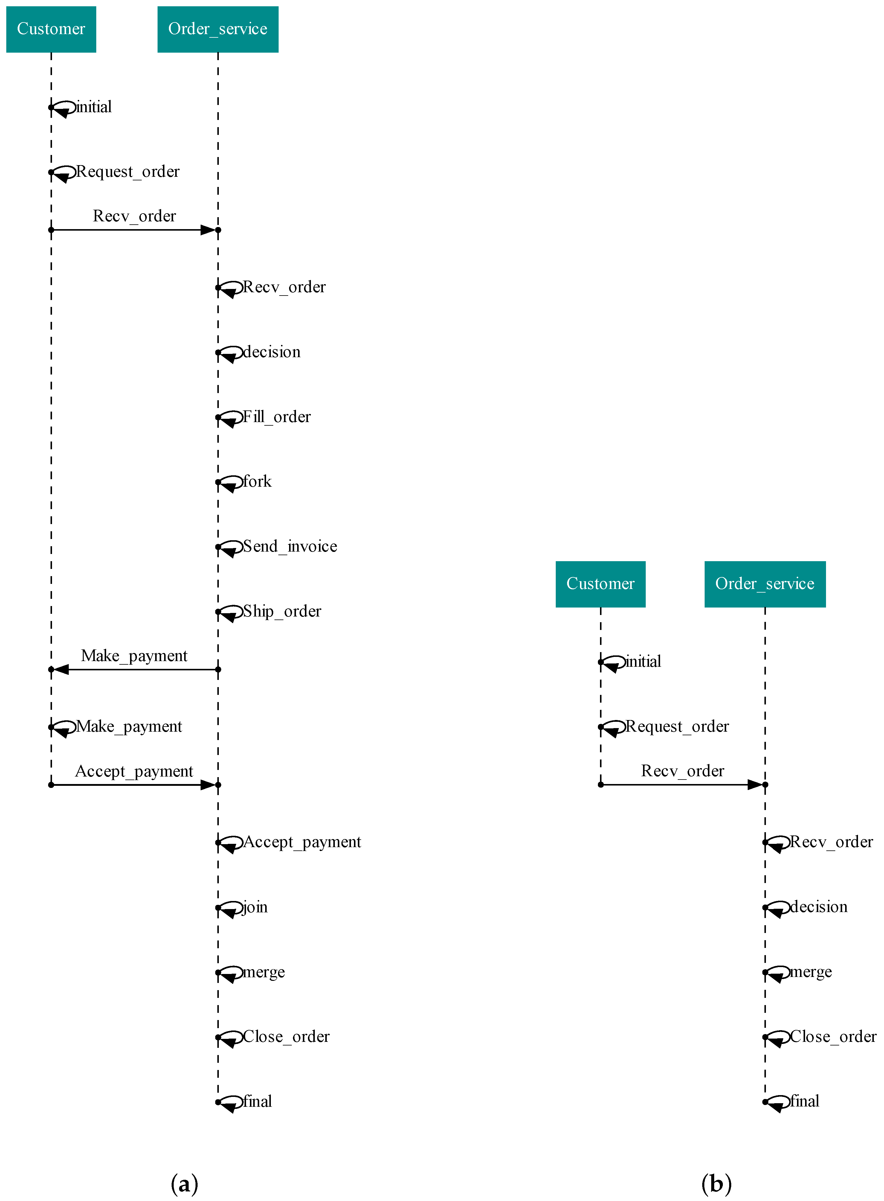
3.4. Case Study: A Shopping Order Processing in an E-Commerce Application

Let us consider the shopping order processing system described in Example 1. The activity diagram depicted in Figure 2 shows the activities involved in the processing of a shopping order. It contains all the common types of nodes and transitions of a UML activity diagram, as explained in Section 2.1. This section presents how this activity diagram can be mapped onto a CCA process and then analysed using the CCA simulation tool ccaPL and the CCA runtime verification tool ccaRV.

3.4.1. Mapping the Activity Diagram onto a CCA Process

The activity diagram in Example 1 can be represented by the tuple

$$(N,T,A,C,mN,mT,mA,mC),$$

as described in Example 2. This tuple is used as input to Algorithm 1 to generate the corresponding CCA process provided in Appendix B. The declaration block that begins with the keyword BEGIN_DECLS and ends with the keyword END_DECLS contains the definition of the context expressions state(n), notEnd(), and decision(n) as stated in lines 2–5 of Algorithm 1 (also see Listing 6). Each actor (the customer and the order service) is represented as an ambient (see Listings 7–10), which is generated by the loop in lines 6–28 of Algorithm 1. Each activity node is represented as a process abstraction (see Table 7, Table 8 and Table 9) local to the ambient corresponding to the actor that performs that activity node. This is carried out by the loop in lines 11–20 of Algorithm 1. The CCA process can be analysed to understand the behaviour of the corresponding activity diagram.

3.4.2. Execution of the Activity Diagram Using ccaPL

The execution of the activity diagram consists of executing the CCA process that the activity diagram is mapped to by Algorithm 1. One can devise various scenarios to test the behaviour of the activity diagram. Let us consider the scenario where an order request is accepted by the order service. The execution output for this case is provided by the communication diagram in Figure 8a, showing all the activities that take place from the moment an order is received to shipment and payment. The top row of the communication diagram shows the actors, which are the customer and the order service. The vertical dashed line leading from an actor represents the timeline of the actor; the time increases from top to bottom. A loop on a timeline indicates the activity performed by the corresponding actor at that time point. An arrow from the timeline of actor A to the timeline of actor B indicates a transfer of flow of control from actor A to actor B. This arrow is labelled with the name of the activity to be executed by B. Now assume that the order request is rejected. To test this scenario, we change accept to reject in the declaration of the context expression decision(n) in the CCA process. The execution output is provided by the communication diagram in Figure 8b. It shows clearly that when the customer submits an order, the order is received and then closed without further processing.

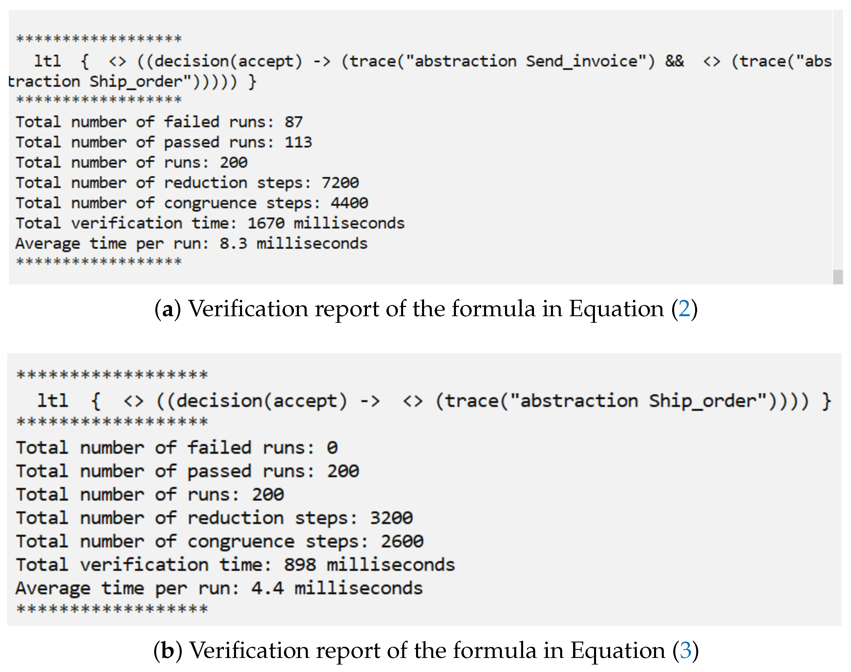
3.4.3. Runtime Verification of the Activity Diagram Using ccaRV

In addition to the execution of an activity diagram, as explained above, one can verify whether the behaviours of an activity diagram satisfy a desired property using the runtime verification tool ccaRV. Let’s consider the property that an invoice must be sent to the customer before the order is shipped. This property is formulated in LTL as in Equation (2).

$$\left.\begin{array}{c}<>\left(\mathtt{d}\mathtt{e}\mathtt{c}\mathtt{i}\mathtt{s}\mathtt{i}\mathtt{o}\mathtt{n}\right(\mathtt{a}\mathtt{c}\mathtt{c}\mathtt{e}\mathtt{p}\mathtt{t})\text{-}>(\mathtt{t}\mathtt{r}\mathtt{a}\mathtt{c}\mathtt{e}("\mathtt{a}\mathtt{b}\mathtt{s}\mathtt{t}\mathtt{r}\mathtt{a}\mathtt{c}\mathtt{t}\mathtt{i}\mathtt{o}\mathtt{n}\mathtt{S}\mathtt{e}\mathtt{n}\mathtt{d}\_\mathtt{i}\mathtt{n}\mathtt{v}\mathtt{o}\mathtt{i}\mathtt{c}\mathtt{e}")\mathtt{\&}\mathtt{\&}\hfill \\ <>\mathtt{t}\mathtt{r}\mathtt{a}\mathtt{c}\mathtt{e}("\mathtt{a}\mathtt{b}\mathtt{s}\mathtt{t}\mathtt{r}\mathtt{a}\mathtt{c}\mathtt{t}\mathtt{i}\mathtt{o}\mathtt{n}\mathtt{S}\mathtt{h}\mathtt{i}\mathtt{p}\_\mathtt{o}\mathtt{r}\mathtt{d}\mathtt{e}\mathtt{r}")\left)\right)\hfill \end{array}\right\}.$$

(2)

This formula says that the process abstraction Send_invoice is called before the process abstraction Ship_order is called (see Table 15) when an order request is accepted. The runtime verification of the activity diagram against this formula using ccaRV produces the verification report in Figure 9a.

The verification report shows that the activity diagram was executed 200 times (we use a large number of runs to increase the chance of catching a violation), and the property was violated in 87 executions (runs). Therefore, the activity diagram allows for an order to be shipped before the invoice is sent to the customer. This is due to the concurrency created by the fork node in the activity diagram. Another property of interest to be checked for this system is that any order (request) accepted is eventually shipped to the customer, i.e.,

<>(decision(accept) -> <>trace("abstraction Ship_order")).

(3)

This time, the verification report in Figure 9b shows that all the 200 runs satisfy the formula in Equation (3). Other properties of the system can be checked in a similar manner.

4. Discussion

Many researchers have investigated the use of formal methods in the verification of UML diagrams. The article [16] reviews the various attempts to define formal semantics for UML and highlights the difficulties in providing complete formal semantics for a complex language like UML. A structural operational semantics for UML activity diagrams is proposed in [17]. The purpose of their semantics is to provide a robust basis for verifying model correctness and to help validate whether a proposed extension of the modelling language is consistent with the standard. Our approach is based on denotational semantics, i.e., an activity diagram is mapped onto a process that describes the activity diagram’s behaviour. The two types of formal semantics are complementary to address various types of system properties. We showed that our approach allows for the execution and the runtime verification of an activity diagram using the CCA toolkit. The relationship between UML activity diagrams and Petri nets is investigated in [18]. They provided a mapping of the basic elements of activity diagrams to Petri nets and discussed the problems arising when trying to extend this approach to some of the advanced features of activity diagrams. This work differs from ours as they are mapping one graphical language to another graphical language. In contrast, our work encodes the behaviour of an activity diagram in a process calculus. An initial work on using CCA to analyse UML activity diagrams is presented in [19], where an algorithm is proposed to translate a UML activity diagram into a CCA process. However, the algorithm they proposed does not work for activity diagrams that contain a loop. Therefore, common iteration control structures like the while-loop or for-loop cannot be handled by the algorithm. This problem is solved in our algorithm by representing activity nodes as process abstractions, which can be called as many times as necessary. The work in [20] also used a process calculus, CSP (communicating sequential processes), to propose an automatic method for verifying the consistency between the UML state machine diagrams and the UML sequence diagrams with hierarchical structure. They provide a process description of state machine diagrams and sequence diagrams and can verify the consistency by checking the trace inclusion of processes using the FDR model checker.

Zhou et al. [21] present the Jasmine tool to detect inconsistencies between the design of a system as UML behaviour diagrams and the implementation of the system in Java using runtime verification. Jasmine takes Java programs under verification and corresponding UML models (including sequence diagrams, activity diagrams, and state machine diagrams) and checks if the programs are consistent with the models. This work is different from ours in the sense that our approach verifies the correctness of the models themselves (in our case, the activity diagrams) through simulation and runtime verification. Ref. [22] presents QMaxUSE, a tool verifying UML class diagrams annotated with a large number of OCL (object constraint language) invariants. To improve the scalability of the tool, they propose a query language that allows users to choose parts of a UML class diagram to be verified. Shah and Grant propose in [8] a precise semantics for a subset of UML class diagrams based on the set theory and the predicate logic. They claim that the approach is particularly relevant for the pedagogy of software engineering and the development of software systems that require a high level of reliability. The verification of the UML class diagrams has been widely investigated, and a systematic review of these works is provided in [9]. This shows the importance of verifying UML diagrams in software engineering.

The authors of [23] proposed a formal transformation of UML activity diagrams into FoCaLiZe, a proof-based formal language. They aimed to verify UML activity diagrams using the Zenon automatic theorem prover. Similar works were carried out by Karmakar et al. [24] and Halder et al. [25]. The former proposed a transformation of UML activity diagrams into Z, a formal specification language based on set theory and predicate logic. The Z notations can then be verified using the Community Z Tools (CZT) suite. Their approach is similar to ours, but they transform UML diagrams to Z manually. The latter converts UML activity diagrams into Event-B specifications, which can be verified using the Rodin tool. The correctness of the UML activity diagram is also investigated in [26] using an approach similar to traditional software testing techniques, which includes unit-level testing, integration-level testing, and system-level testing. A study on extracting UML activity diagrams and UML use case diagrams from the requirement specification is proposed in [27]. They use text mining techniques to extract the UML diagrams. This work is complementary to ours as it can help to extract a UML activity diagram from the requirement specification document and then apply our technique to transform that UML activity diagram into a CCA process, which is then analysed (using ccaPL and ccaRV tools) to detect defects or inconsistencies in the requirement specification.

5. Conclusions

This paper proposes an approach to execute and verify UML activity diagrams based on the calculus of context-aware ambients (CCA). An algorithm is developed that maps any UML activity diagram onto a CCA process, which describes the behaviours of the UML activity diagram. This process can be executed (using the CCA interpreter ccaPL) upon various scenarios in order to better understand the behaviours of the UML activity diagram. This algorithm can be thought of as a semantics mapping for UML activity diagrams. The algorithm is implemented in Python to automate the mapping task. In addition to being able to execute UML activity diagrams, a runtime verification tool, ccaRV, is implemented to enable the verification of a UML activity diagram against a desired property specified as a formula in linear temporal logic (LTL). The syntax and the semantics of LTL are extended to include the notion of context expression and other new predicates, such as trace() for recording execution traces. A case study is used to illustrate how the proposed approach can be applied in practice. Compared to the model-checking techniques, runtime verification is more scalable as it checks just a single execution path. Although runtime verification does not guarantee full system correctness, it is effective in detecting design flaws [13,14]. Another limitation of this work is that it is not possible to prove formally the correctness of the proposed semantics for UML activity diagrams because the original documentation of UML [1] does not provide formal semantics to carry out a comparison.

In future work, we will extend the proposed approach to more complex modelling languages like the business process modelling Language (BPML). We will also investigate how the approach proposed in this paper can be applied to the verification of activity diagrams for IoT systems.

References

1. Object Management Group. OMG Unified Modeling Language (OMG UML), Superstructure. Version 2.4.1; Object Management Group: Milford, PA, USA, 2011. [Google Scholar]
2. ISO/IEC 19501:2005; Information Technology—Open Distributed Processing—Unified Modeling Language (UML) Version 1.4.3. International Organization for Standardization: Geneva, Switzerland, 2005.
3. Li, X.; Liu, Z.; Jifeng, H. A formal semantics of UML sequence diagram. In Proceedings of the 2004 Australian Software Engineering Conference. Proceedings., Melbourne, Australia, 13–16 April 2004; pp. 168–177. [Google Scholar] [CrossRef]
4. Fernandes, F.; Song, M.A. UML-Checker: An Approach for Verifying UML Behavioral Diagrams. J. Softw. 2014, 9, 1229–1236. [Google Scholar] [CrossRef]
5. Lima, V.; Talhi, C.; Mouheb, D.; Debbabi, M.; Wang, L.; Pourzandi, M. Formal Verification and Validation of UML 2.0 Sequence Diagrams using Source and Destination of Messages. Electron. Notes Theor. Comput. Sci. 2009, 254, 143–160. [Google Scholar] [CrossRef]
6. Mokhati, F.; Gagnon, P.; Badri, M. Verifying UML Diagrams with Model Checking: A Rewriting Logic Based Approach. In Proceedings of the Seventh International Conference on Quality Software (QSIC 2007), Portland, OR, USA, 11–12 October 2007; pp. 356–362. [Google Scholar]
7. Le, L.C. A Method for Modeling and Verifying of UML 2.0 Sequence Diagrams using SPIN. J. Sci. Technol. Inf. Secur. 2020, 1, 20–28. [Google Scholar] [CrossRef]
8. Shah, K.; Grant, E. Towards Simplifying and Formalizing UML Class Diagram Generalization/Specialization Relationship with Mathematical Set Theory. In Proceedings of the 6th International Conference on Information System and Data Mining, ICISDM ’22, Silicon Valley, CA, USA, 27–29 May 2022; pp. 89–94. [Google Scholar]
9. Shaikh, A.; Hafeez, A.; Wagan, A.A.; Alrizq, M.; Alghamdi, A.; Reshan, M.S.A. More Than Two Decades of Research on Verification of UML Class Models: A Systematic Literature Review. IEEE Access 2021, 9, 142461–142474. [Google Scholar] [CrossRef]
10. Siewe, F.; Zedan, H.; Cau, A. The Calculus of Context-aware Ambients. J. Comput. Syst. Sci. 2011, 77, 597–620. [Google Scholar] [CrossRef]
11. Siewe, F. ccaPL: A CCA Programming Environment. Available online: https://fsiewe.afrilocode.net/CCA/index.html (accessed on 23 November 2023).
12. AT&T Labs-Research. Graphviz Distribution. Available online: http://www.research.att.com/sw/tools/graphviz/download.html (accessed on 23 November 2023).
13. Havelund, K.; Peled, D. Runtime Verification: From Propositional to First-Order Temporal Logic. In Runtime Verification; Colombo, C., Leucker, M., Eds.; Springer: Cham, Switzerland, 2018; pp. 90–112. [Google Scholar]
14. Bartocci, E.; Falcone, Y.; Francalanza, A.; Reger, G. Introduction to Runtime Verification. In Lectures on Runtime Verification: Introductory and Advanced Topics; Bartocci, E., Falcone, Y., Eds.; Springer International Publishing: Cham, Switzerland, 2018; pp. 1–33. [Google Scholar]
15. Havelund, K.; Roşu, G. Runtime Verification—17 Years Later. In Runtime Verification; Colombo, C., Leucker, M., Eds.; Springer: Cham, Switzerland, 2018; pp. 3–17. [Google Scholar]
16. Broy, M.; Cengarle, M.V. UML formal semantics: Lessons learned. Softw. Syst. Model. 2011, 10, 441–446. [Google Scholar] [CrossRef]
17. Daw, Z.; Cleaveland, R. An extensible formal semantics for UML activity diagrams. arXiv 2016, arXiv:1604.02386. [Google Scholar]
18. Störrle, H.; Hausmann, J.H. Towards a formal semantics of UML 2.0 activities. In Proceedings of the Software Engineering 2005, Essen, Germany, 8–11 March 2005; Liggesmeyer, P., Pohl, K., Goedicke, M., Eds.; Gesellschaft für Informatik e.V.: Bonn, Germany, 2005; pp. 117–128. [Google Scholar]
19. Siewe, F. Towards the Formal Analysis of UML Activity Diagrams in a Calculus of Context-aware Ambients. In Proceedings of the 2023 IEEE 47th Annual Computers, Software, and Applications Conference (COMPSAC), Torino, Italy, 27–29 June 2023; pp. 1691–1696. [Google Scholar]
20. Matsumoto, A.; Yokogawa, T.; Amasaki, S.; Aman, H.; Arimoto, K. Synthesis and Consistency Verification of UML Sequence Diagrams with Hierarchical Structure. Inf. Eng. Express 2020, 6, 1–19. [Google Scholar]
21. Zhou, Z.; Wang, L.; Cui, Z.; Chen, X.; Zhao, J. Jasmine: A Tool for Model-Driven Runtime Verification with UML Behavioral Models. In Proceedings of the 2008 11th IEEE High Assurance Systems Engineering Symposium, Nanjing, China, 3–5 December 2008; pp. 487–490. [Google Scholar]
22. Wu, H. QMaxUSE: A new tool for verifying UML class diagrams and OCL invariants. Sci. Comput. Program. 2023, 228, 102955. [Google Scholar] [CrossRef]
23. Abbas, M.; Rioboo, R.; Ben-Yelles, C.B.; Snook, C.F. Formal modeling and verification of UML Activity Diagrams (UAD) with FoCaLiZe. J. Syst. Archit. 2021, 114, 101911. [Google Scholar] [CrossRef]
24. Karmakar, R.; Bera, P.; Dutta, S. FMSG: A framework for modeling and verification of a smart grid. Sadhana—Acad. Proc. Eng. Sci. 2024, 49, 131. [Google Scholar] [CrossRef]
25. Halder, A.; Karmakar, R. Mapping UML Activity Diagram into Z Notation. Lect. Notes Data Eng. Commun. Technol. 2022, 96, 301–318. [Google Scholar]
26. Xu, Z.; Sun, F.; Zhang, W. Research on Activity Diagram Testing method based on UML Testing Profile. In Proceedings of the 2024 6th International Conference on Electronic Engineering and Informatics (EEI), Chongqing, China, 28–30 June 2024; pp. 434–439. [Google Scholar]
27. Muqsith, M.F.; Priyadi, Y.; Astuti, W. UML Artifact Extraction for Activity Diagram Based on Step Performed Using Text Mining: Case Study of SRS Sipranta Application. In Proceedings of the 2023 3rd International Conference on Electronic and Electrical Engineering and Intelligent System (ICE3IS), Yogyakarta, Indonesia, 9–10 August 2023; pp. 246–251. [Google Scholar]
Figure 1. Elements of an activity diagram.
Software 04 00004 g001
Figure 2. An activity diagram for shopping order processing.
Software 04 00004 g002
Figure 3. The ccaPL tool.
Software 04 00004 g003
Figure 4. Textual execution trace.
Software 04 00004 g004
Figure 5. Graphical execution traces.
Software 04 00004 g005
Figure 6. The ccaRV tool.
Software 04 00004 g006
Figure 7. Examples of runtime verification reports for the simple access control system of Section 2.2.5. The screenshot at the top (i.e., (a)) shows a verification report for an RFID number of 166. The screenshot at the bottom (i.e., (b)) shows a verification report for an RFID number of 70.
Software 04 00004 g007
Figure 8. Examples of execution traces (in the form of communication diagrams) for the activity diagram of Figure 2: (a) order request is accepted and (b) order request is rejected.
Software 04 00004 g008
Figure 9. Examples of runtime verification reports for the activity diagram of Figure 2 against (a) the formula in Equation (2) and (b) the formula in Equation (3).
Software 04 00004 g009