RbfCon: Construct Radial Basis Function Neural Networks with Grammatical Evolution

Abstract

Radial basis function networks are considered a machine learning tool that can be applied on a wide series of classification and regression problems proposed in various research topics of the modern world. However, in many cases, the initial training method used to fit the parameters of these models can produce poor results either due to unstable numerical operations or its inability to effectively locate the lowest value of the error function. The current work proposed a novel method that constructs the architecture of this model and estimates the values for each parameter of the model with the incorporation of Grammatical Evolution. The proposed method was coded in ANSI C++, and the produced software was tested for its effectiveness on a wide series of datasets. The experimental results certified the adequacy of the new method to solve difficult problems, and in the vast majority of cases, the error in the classification or approximation of functions was significantly lower than the case where the original training method was applied.

1. Introduction

A variety of real-world problems can be considered as classification and regression problems, handled by machine learning models that have been thoroughly studied in the literature. Such problems arise in physics [1,2], chemistry [3,4], economics [5,6], medicine [7,8], etc. One common machine learning model that is applied in many areas is the radial basis function (RBF) neural network [9,10]. These neural networks are commonly formed using the following mathematical expression:

$$y\left(\overrightarrow{x}\right)=\sum _{i=1}^k{w}_i\varphi \left(∥\overrightarrow{x}-\overrightarrow{c_i}∥\right)$$

(1)

The following notation is used in Equation (1):

• The vector $\overrightarrow{x}$ represents the input pattern with dimension d.
• The parameter k stands for the number of weights of the model. These weights are represented by vector $\overrightarrow{w}$.
• The vectors $\overrightarrow{c_i},i=1,\dots ,k$ represent the so-called centers of the network.
• The final output of the model for the input pattern $\overrightarrow{x}$ is denoted by $y\left(\overrightarrow{x}\right)$.
• The function $\varphi \left(x\right)$ in most cases is represented by the Gaussian function defined as

  $$\varphi \left(x\right)=exp\left(-{\displaystyle \frac{{\left(x-c\right)}^2}{{\sigma }^2}}\right)$$

  (2)
  This function is selected as the output function since the output value $\varphi \left(x\right)$ uses only the distance of vectors x and c.

RBF neural networks were extensively used and studied in recent literature and, among others, can find applications in problems derived from physics [11,12], robotics [13,14], security problems [15,16], image processing [17,18], etc. Due to the widespread use of these machine learning models and their use in both classification and data fitting problems, a number of techniques were presented in recent years that seek to more accurately identify their parameters. Such methods include techniques used to initialize the parameters of these models [19,20,21] or pruning methods for the optimal adaptation of the architecture of these models [22,23,24]. Also, global optimization methods were proposed to estimate the optimal set of parameters of RBF networks in a series of research papers [25,26,27].

Furthermore, a discussion on the kernel widths of RBF networks is provided in the work of Benoudjit et al. [28]. Paetz proposed a method [29] that can reduce the number of neurons in RBF networks with dynamic decay adjustment in order to increase the generalization abilities of these networks. Yu et al., in their work [30], proposed an incremental design technique for RBF networks in order to estimate the optimal architecture of these networks. Moreover, Alexandridis et al. [31] proposed the incorporation of the Particle Swarm Optimization method to effectively estimate the weights of RBF networks. Also, Neruda et al. [32] provided a detailed comparison of methods used to estimate the parameters of RBF networks. Additionally, due to the widespread usage of parallel programming techniques, a series of techniques that exploit parallel computing units were suggested in recent years for RBF network training [33,34].

In most cases, the set of parameters of the model is estimated using a two-phase method: during the first phase, the set of centers and variances in Equation (1) are calculated using the K-means algorithm [35]. In the second phase, the set of weights $\overrightarrow{w}$ is obtained by solving a linear system of equations. Although the previous procedure is capable of estimating the optimal set of parameters in a very short time, it, nevertheless, has a number of problems with regard to numerical stability, the accurate determination of the number of weights, over-fitting problems, etc. To calculate these parameters with the classical calculation method, it is necessary to solve a system of equations, but in many cases, the solution of such a system leads to numerical problems as determinants appear with a value quite close to zero. To tackle such problems, a novel method was proposed in this study that constructs the optimal architecture of RBF networks using a method that incorporates the Grammatical Evolution procedure [36]. The proposed technique is able to estimate both the optimal architecture of the neural network and the numerical values of its parameters, and in this study, both the algorithm used and the software created for this process, which is freely available from the internet, are presented in detail.

The software proposed in this work is fully implemented in the programming language ANSI C++ and is executable with a series of command line parameters with which the user can efficiently process the datasets at their disposal. The contribution of the proposed technique and the implemented software can be summarized as follows:

• The method can efficiently construct the structure of RBF networks and achieve optimal adjustment of their parameters.
• The resulting networks do not have the numerical problems caused by the traditional training technique of RBF networks.
• The created software provides an easy user interface for performing experiments and can be installed on almost any operating system.

The rest of this article is divided into the following sections: in Section 2, the proposed methodology and the used software are thoroughly discussed; in Section 3, the datasets incorporated in the conducted experiments are listed, followed by the experimental results; in Section 4, a discussion on the experimental results is provided; and finally, in Section 5, a series of conclusions is presented.

2. Materials and Methods

The original training method of RBF networks is presented here followed by the detail presentation of the Grammatical Evolution procedure. Afterwards, the proposed method is fully described accompanied by a full working example of the proposed software.

2.1. The Original Training Procedure of RBF Neural Networks

The typical training procedure of an RBF network $y\left(x\right)={\sum }_{i=1}^k{w}_i\varphi \left(∥x-c_i∥\right)$ involves two major steps: In the first step, the centers $\overrightarrow{c_i}$ and the variances are calculated using the K-means procedure, which is described in Algorithm 1. During the second step, a system of equations should be solved to calculate the values for weights $w_i,i=1,\dots ,k$ as follows:

• Set $W=w_{kj}$ the matrix of k weights, $\Phi ={\varphi }_j\left(x_i\right)$, and $T=\left\{t_i\right\}$, where $t_i,i=1,\dots ,M$ are the expected values for input patterns $x_i$.
• Solve

  $${\Phi }^T\left(T-\Phi W^T\right)=0$$

  (3)

  $$W^T={\left({\Phi }^T\Phi \right)}^{-1}{\Phi }^{T}T={\Phi }^{†}T$$

  (4)
  The matrix ${\Phi }^{†}={\left({\Phi }^T\Phi \right)}^{-1}{\Phi }^T$ denotes the the pseudo-inverse of $\Phi$, with

  $${\Phi }^{†}\Phi =I$$

  (5)

Algorithm 1 The used K-means Algorithm

Initialization (a) Set k the number of centers. (b) Read the patterns of the training dataset $x_i,i=1,\dots ,M$ (c) Set $S_j=\varnothing$, from $j=1,\dots ,k$. For every pattern $x_i,i=1,\dots ,M$ do (a) Set $j^{*}={\mathrm{argmin}}_{m=1}^k\left\{D\left(x_i,c_m\right)\right\}$ where the variable $j^{*}$ denotes the nearest center from $x_i$ (b) Set $S_{j^{*}}=S_{j^{*}}\cup \left\{x_i\right\}$. End For For each center $c_j,j=1..k$ do (a) Calculate and denote as $M_j$ the number of samples in $S_j$ (b) Update the center $c_j$ as $$c_j={\displaystyle \frac{1}{M_j}}\sum _{x_i\in S_j}{x}_i$$ End For If the centers $c_j$ did not change then terminate else goto step 2

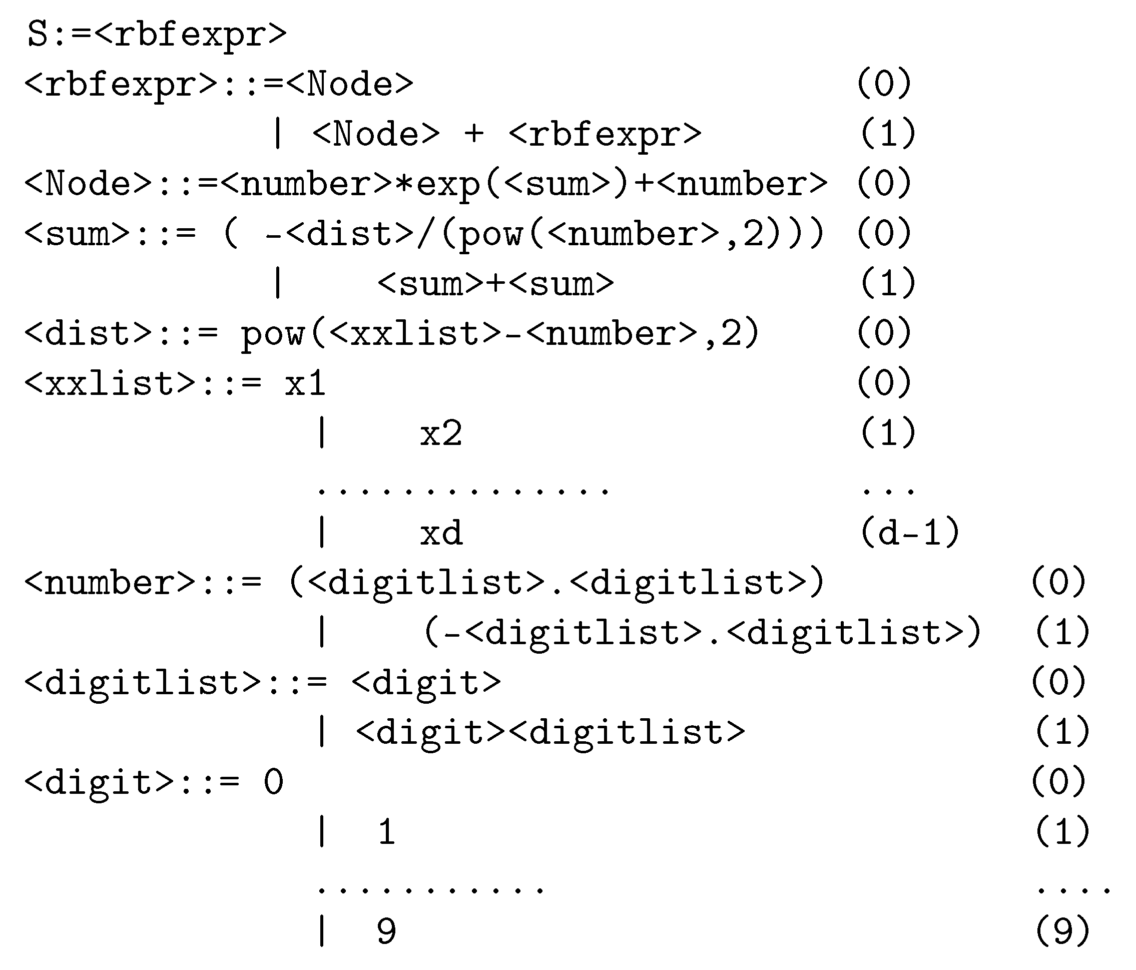
2.2. The Used Construction Procedure

The Grammatical Evolution procedure is able to construct programs in the provided Backus Naur Form (BNF) grammar [37] with the assistance of a genetic algorithm that utilizes integer chromosomes. These chromosomes represent rule numbers from the underlying grammar, and the method was used successfully in a series of cases, such as: trigonometric problems [38], production of music [39], construction of neural networks [40,41], video games [42,43], credit classification [44], network security [45], etc. Furthermore, many researchers developed and published a series of software regarding Grammatical Evolution, such as the GEVA [46] which suggests a GUI environment, a statistical software written in R named gramEvol [47], a Matlab toolbox named GeLab [48], the GenClass software used in classification problems [49], the QFc software [50] used to construct artificial features, etc.

The proposed procedure constructs the structure of an RBF neural network using Grammatical Evolution and BNF grammar and an appropriately modified genetic algorithm [51,52] that guides the course of the procedure. The grammar functions used in the Grammatical Evolution procedure are BNF grammar expressed as sets $G=\left(N,T,S,P\right)$, where

• The symbol N stands for the set of non-terminal symbols;
• The symbol T represents the set of terminal symbols;
• S is a non-terminal symbol, used as the start symbol of the grammar;
• P is the set of production rules that are used to produce terminal symbols from non-terminal symbols.

For each chromosome, Grammatical Evolution initiates from the symbol S, and through a series of production steps, it creates programs with terminal symbols by substituting non-terminal symbols with the right hand of the selected production rule. The selection of the production rule is accomplished in two steps:

• Obtain the next element V from the under-processing chromosome.
• Select the next production rule according to the equation, Rule = V mod $N_R$, where the quantity $N_R$ stands for the total number of production rules for the non-terminal symbol that is under processing.

The required BNF grammar for the current algorithm is outlined in Figure 1. The terminal symbol exp represents the function $exp\left(x\right)$, and the terminal symbol pow stands for the power operator $x^y$.

The steps of the algorithm used to create RBF neural networks are listed below:

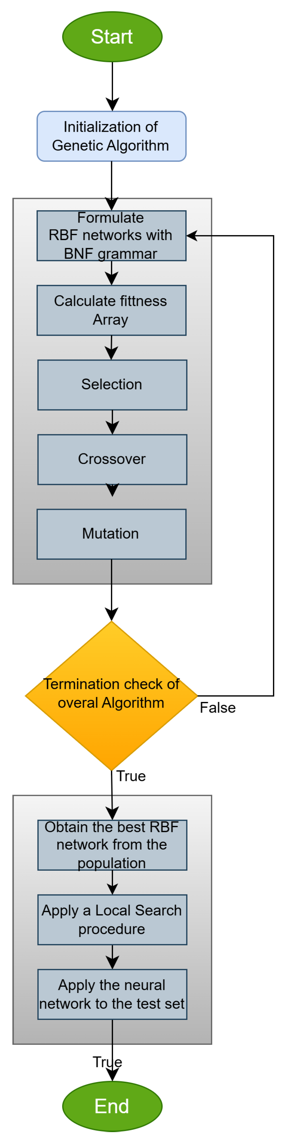
• Initialization Step.

  (a)

  Set the number of chromosomes $N_c$ and the number of allowed generations $N_g$.

  (b)

  Set the selection rate of the genetic algorithm, denoted as $p_c$ where $p_c\le 1$.

  (c)

  Set the mutation rate of the genetic algorithm, denoted as $p_m$, with $p_m\le$1.

  (d)

  Initialize the chromosomes as sets of positive random integers.

  (e)

  Set k = 0, the generation number.

• Main loop step.

  (a)

  Evaluate fitness.

  • For every chromosome $C_i,i=1,\dots ,N_c$ create the corresponding neural network using the grammar of Figure 1. Denote this network as $y_i\left(x\right)$.
  • Compute the fitness $f_i$ for the train set as

    $$f_i=\sum _{j=1}^M{\left(y_i\left({\overrightarrow{x}}_j\right)-t_j\right)}^2$$

    (6)

    The set $\left(\overrightarrow{x_j},t_j\right),j=1,\dots ,M$ represents the train dataset of the objective problem.

  (b)

  Apply the selection operator. A sorting of the chromosomes is performed according to their fitness values. The best $\left(1-p_s\right)\times N_c$ of them are copied without changes to the next generation. The rest of the chromosomes will be replaced by new chromosomes produced during the crossover procedure.

  (c)

  Apply the crossover operator. During this procedure, a series of $p_s\times N_c$ offsprings will be produced. For each pair of offsprings denoted as $\tilde{z}$ and $\tilde{w}$, two chromosomes $(z,w)$ should be selected from the original population using tournament selection. The production of the new chromosomes is conducted using the one-point crossover procedure. An example of this process is graphically outlined in Figure 2.

  (d)

  Perform mutation. For each element of every chromosome, randomly draw a number $r\in \left[0,1\right]$. If $r\le p_m$, then the corresponding element is replaced by a new randomly produced element.

  (e)

  Set k = k + 1.

• Check for the termination step. If $k\le N_g$, then go to step 2.
• Local Optimization step. Obtain the chromosome $C^{*}$ and produce the corresponding RBF neural network $y^{*}\left(x\right)$. The parameters of this neural network are obtained by minimizing with some local search procedure the training error defined as

  $$E\left(y^{*}\left(x\right)\right)=\sum _{j=1}^M{\left(y^{*}\left({\overrightarrow{x}}_j\right)-t_j\right)}^2$$

  (7)
• Application in test set. Apply the final model $y^{*}\left(x\right)$ to the test dataset and report the test error.

The steps of the proposed method are also outlined as a flowchart in Figure 3.

2.3. Installation Procedure

The software was coded entirely in ANSI C++, and the software is available freely from the following URL: https://github.com/itsoulos/RbfCon (accessed on 14 November 2024). The user should install the QT Library, which is accessible from https://qt.io (accessed on 14 November 2024) in order to compile the software. After downloading the RbfCon-master.zip file, the user should execute the following commands, under any Unix-based system:

• unzip RbfCon-master.zip;
• cd RbfCon-master;
• qmake (or qmake-qt5 in some Linux installations);
• make.

For Windows systems, the user alternatively could install the software using the RBFCON.msi located in the distribution, which is an installation file that installs the software without the need for the QT Library.

2.4. The Main Executable RbfCon

The final outcome of the compilation has a series of command line parameters that the user may adjust. The list of these parameters is as follows:

• $--$trainfile=<filename> The string parameter filename determines the name of the file containing the training dataset for the software. The user is required to provide this parameter to start the process. The format for this file is shown in Figure 4. The first number denoted as D in this figure determines the dimension of the input dataset, and the second number denoted as M represents the number of input patterns. Every line in the file contains a pattern and the required desired output.
• $--$testfile=<filename> The string parameter filename stands for the name of the test dataset used by the software. The user should provide at least the parameters trainfile and testfile in order to initiate the method. The format of the test dataset is the same as the training dataset.
• $--$chromosome_count=<count> This integer parameter denotes the number of chromosomes in the genetic algorithm (parameter $N_c$ of the algorithm). The default value for this parameter is 500.
• $--$chromosome_size=<size> The integer parameter size determines the size of each chromosome for the Grammatical Evolution process. The default value for this parameter is 100.
• $--$selection_rate=<rate> The double precision parameter rate stands for the selection rate of the Grammatical Evolution process. The default value for this parameter is 0.10 (10%).
• $--$mutation_rate=<rate> The double precision parameter rate represents the mutation rate for the Grammatical Evolution process. The default value for this parameter is 0.05 (5%).
• $--$generations=<gens> The integer parameter gens stands for the maximum number of allowed generations for the Grammatical Evolution procedure (parameter $N_g$ of the current algorithm). The original value is 500.
• $--$local_method=<method> The used local optimization method will be applied to the parameters of the RBF model when the Grammatical Evolution procedure finished. The available local optimization methods are as follows:

  (a)

  lbfgs. The method L-BFGS can be considered a variation in the Broyden–Fletcher–Goldfarb–Shanno (BFGS) optimization technique [53], which utilizes a minimum amount of memory. This optimization method was used in many cases, such as image reconstruction [54], inverse eigenvalue problems [55], seismic problems [56], training of deep neural networks [57], etc. Also, the series of modifications that take advantage of modern parallel computing systems were proposed [58,59,60].

  (b)

  bfgs. The BFGS variant of Powell was used here [61], when this option is enabled.

  (c)

  adam. This option denotes the application of the Adam optimizer [62] as the local optimization algorithm.

  (d)

  gradient. This option represents the usage of the Gradient Descent method [63] as the local optimization algorithm.

  (e)

  none. With this option, no local optimization method will be used after the Genetic Algorithm is terminated.

• $--$iterations=<iters> This integer parameter determines the number of consecutive applications of the proposed technique to the original dataset. The default value is 30.

2.5. Example of Execution

As a fully working example, consider the Wdbc dataset [64], which is located under EXAMPLES subdirectory. This dataset is used for the detection of breast tumors. An example of execution could be the following:

./RbfCon --trainfile=EXAMPLES/wdbc.train --testfile=EXAMPLES/wdbc.test --iterations=2

The output of this command is shown in Algorithm 2.

Algorithm 2 The output of the example run

Iteration:    1 TRAIN ERROR:          20.40039584 Iteration:    1 TEST  ERROR:        0.07733519754 Iteration:    1 CLASS ERROR:                 9.12% Iteration:    1 SOLUTION:    ((6.711)*(exp((−((pow(x13 − (−97.73),2))+   ((pow(x23 − (43.7),2))+((pow(x23 − (84.7),2))+   (pow(x23 − (91.3),2))))))/(2*pow((60.1),2))))+   (−0.0099969))+((−0.39)*(exp((−((pow(x25 − (9.336),2))+   ((pow(x18 − (6.8),2))+(pow(x4 − (6.52),2)))))/(2*pow((711.5),2))))+   (0.00185452))+((3.7)*(exp((−(pow(x3 − (−6.8),2)))/(2*pow((2.3),2))))+   (−0.001))+((−5.8)*(exp((−(pow(x2 − (−99969.10),2)))/   (2*pow((6342.3747),2))))+(−0.002)) Iteration:    2 TRAIN ERROR:          16.06705417 Iteration:    2 TEST  ERROR:        0.05654528154 Iteration:    2 CLASS ERROR:                 4.56% Iteration:    2 SOLUTION:    ((4.4)*(exp((−((pow(x27 − (3.6),2))+   (pow(x23 − (8.9893),2))))/(2*pow((49.9),2))))+(−0.004))+   ((−2.09)*(exp((−((pow(x23 − (−9.1),2))+   ((pow(x30 − (−40.4),2))+((pow(x4 − (98.5),2))+   (pow(x22 − (−4.4),2))))))/(2*pow((189.9),2))))+(0.007))+   ((−9.8)*(exp((−((pow(x2 − (24.4),2))+((pow(x28 − (2.04),2))+   (pow(x27 − (9.11),2)))))/(2*pow((3.1),2))))+(0.009))+   ((−67.49)*(exp((−(pow(x10 − (−2629940.4),2)))/(2*pow((098.5),2))))+(0.0094)) Average Train Error:          18.23372501 Average Test  Error:        0.06694023954 Average Class Error:                 6.84%

The program prints the train error, the test error, and the classification for every run, as well as the averages for these values. Also, in each execution, the main program shows the constructed RBF network as a string value.

The basic elements that the software requires when initializing the process are essentially the file containing the training data and the file containing the test data. Both of these files must have the proposed structure and the same number of patterns. The user can change other elements of the algorithm, such as the number of chromosomes, through a series of parameters, but this is not required. At the end, the software will display the average training error, the average error in the test set, and the average classification error.

3. Results

The new technique can be used to construct RBF networks for both classification and data fitting problems. For this reason, datasets covering many scientific areas are used from the following websites:

• The UCI repository, https://archive.ics.uci.edu/ (accessed on 14 November 2024) [65];
• The Keel repository, https://sci2s.ugr.es/keel/datasets.php (accessed on 14 November 2024) [66];
• The Statlib URL ftp://lib.stat.cmu.edu/datasets/index.html (accessed on 14 November 2024).

3.1. The Used Datasets

The following list contains the used classification datasets for the the conducted experiments:

• Appendicitis, a medical dataset that was studied in [67,68]. This problem has two distinct classes.
• Alcohol, a dataset related to alcohol consumption [69]. This dataset contains four distinct classes.
• Australian, an economic dataset [70]. The number of classes for this dataset is two.
• Bands, related to problems that occur in printing [71]. It has two classes.
• Cleveland, a medical dataset proposed in a series of research papers [72,73]. This dataset has five distinct classes.
• Dermatology, which is also a medical dataset originated in [74]. It has six classes.
• Ecoli, that is related to problems regarding proteins [75]. It has eight classes.
• Fert, used in demographics. It has two distinct classes.
• Haberman, a medical dataset related to the detection of breast cancer. This dataset has two classes.
• Hayes-roth dataset [76]. This dataset has three classes.
• Heart, a medical dataset about heart diseases [77]. This dataset has two classes.
• HeartAttack, which is a medical dataset related to heart diseases. It has two distinct classes.
• Hepatitis, a dataset used for the detection of hepatitis.
• Housevotes, used for the Congressional voting in USA [78].
• Ionosphere, used for measurements from the ionosphere [79,80]. It has two classes.
• Liverdisorder, which is a medical dataset [81,82] with two classes.
• Lymography [83], which has four classes.
• Magic, this dataset contains generated data to simulate registration of high energy gamma particles [84]. It has two classes.
• Mammographic, a medical dataset related to the presence of breast cancer [85].
• Parkinsons, a dataset used for the detection of Parkinson’s disease [86,87].
• Pima, a medical dataset that was useful for the detection of diabetes [88].
• Popfailures, a dataset contains climate measurements [89]. It has two classes.
• Regions2, a medical dataset that contains measurements from liver biopsy images [90]. It has five classes.
• Ring, which is a problem with 20 dimensions and two classes, related to a series of multivariate normal distributions.
• Saheart, a medical dataset related to heart diseases with two classes [91].
• Statheart, which is a also a medical dataset related to heart diseases.
• Spambase, a dataset used to detect spam emails from a large database. The dataset has two distinct classes.
• Spiral, an artificial dataset with two classes.
• Student, a dataset contains measurements from various experiments in schools [92].
• Tae, this dataset consist of evaluations of teaching performance. It has three classes.
• Transfusion, which is a medical dataset [93].
• Wdbc, a medical dataset used to detect the presence of breast cancer [94,95].
• Wine, a dataset contains measurements about the quality of wines [96,97], with three distinct classes.
• EEG dataset, which is a medical dataset about EEG measurements studied in a series of papers [98,99]. The following cases were obtained from this dataset: Z_F_S, ZO_NF_S, Z_O_N_F_S and ZONF_S.
• Zoo, which used to detect the class of some animals [100]. It contains seven classes.

The next list provided the regression datasets that was incorporated during the conducted experiments:

• Abalone, a dataset that used to predict the age of abalones with 8 features.
• Airfoil, a dataset provided by NASA [101] with 5 features.
• Auto, a dataset used to predict the fuel consumption with 7 features.
• BK, that contains measurements from a series of basketball games with 4 features.
• BL, a dataset used to record electricity experiments with 7 features.
• Baseball, a dataset with 16 features used to estimate the income of baseball players.
• Concrete, a dataset with 8 features used in civil engineering [102].
• DEE, a dataset with 6 featured that was to predict the electricity cost.
• FA, that contains measurements about the body fat with 18 features.
• HO, a dataset originated in the STATLIB repository with 13 features.
• Housing, used to predict the price of houses [103] with 13 features.
• Laser, which is a dataset with 4 features. It has been used in various laser experiments.
• LW, a dataset with 9 features used to record the weight of babies.
• MB, a dataset provide by from Smoothing Methods in Statistics [104] with 2 features.
• Mortgage, an economic dataset from USA with 15 features.
• NT, a dataset with 2 features used to record body temperatures [105].
• Plastic, a dataset with 2 features used to detect the pressure on plastics.
• PL, a dataset with 2 features provided by the STATLIB repository.
• Quake, a dataset used to measure the strength of earthquakes with 3 features.
• SN, a dataset that provides experimental measurements related to trellising and pruning. This dataset has 11 features.
• Stock, a dataset with 9 features used to approximate the prices of various stocks.
• Treasury, an economic dataset from USA that contains 15 features.
• TZ, which is a dataset originated in the STATLIB repository. It has 60 features.

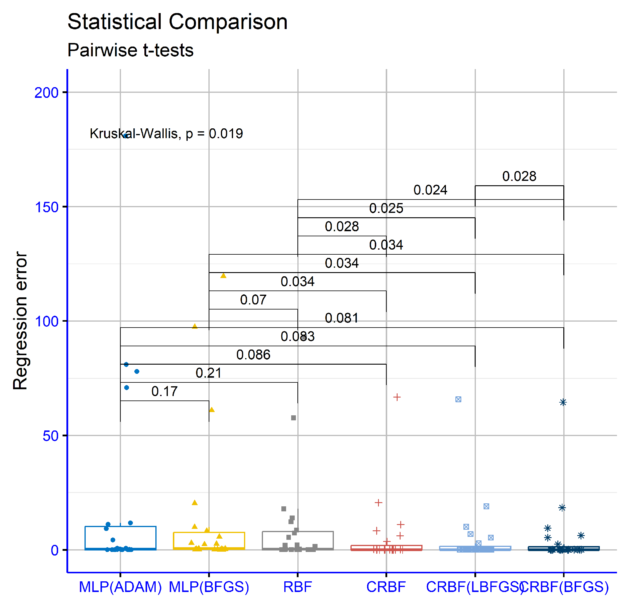
3.2. Experimental Results

The implementation of the machine learning methods that participated in the conducted experiments was made using ANSI C++. The experiments were conducted 30 times, and the average classification or regression error as measured on the test was recorded. The classification error is measured as follows:

$$E_C\left(M\left(x\right)\right)=100\times {\displaystyle \frac{{\sum }_{i=1}^N\left(\mathrm{class}\left(M\left(x_i\right)\right)-y_i\right)}{N}}$$

(8)

where $M\left(x\right)$ denotes the used machine learning model, and set T denotes the train dataset. On the other hand, the regression error is calculated as follows:

$$E_R\left(M\left(x\right)\right)={\displaystyle \frac{{\sum }_{i=1}^N{\left(M\left(x_i\right)-y_i\right)}^2}{N}}$$

(9)

The well-known technique of ten-fold cross-validation was incorporated for the validation of the experimental results. The experiments were executed on an AMD Ryzen 5950X with 128 GB of RAM, running as the operating system the Debian Linux. The values for the parameters of the algorithm are presented in

Table 1. The values for the experimental parameters.

Parameter	Value
chromosome_count	500
chromosome_size	100
selection_rate	0.1
mutation_rate	0.05
generations	500

.

This particular set of parameters was used in a multitude of scientific publications and can be considered as a compromise between the efficiency of an evolutionary process such as the one proposed in this work and the speed necessary to extract the results of its application within a reasonable time.

The experimental results from the application of various method on the classification datasets are shown in Table 2 and for the regression datasets in Table 3. For all tables, the following notation was used:

• The column MLP(ADAM) represents the usage of the ADAM optimization method [62] to train an artificial neural network with $k=10$ processing nodes.
• The column MLP(BFGS) stands for the usage of the BFGS optimization method [61] in the training process of an artificial neural network with $k=10$ processing nodes.
• The column RBF denotes the usage of the original two-phase method for the training of an RBF neural network with $k=10$ weights. This method was described previously in Section 2.1.
• The column CRBF stands for the utilization of the current software using the parameters of Table 1, and as local search procedure, the none option was selected.
• The column CRBF(LBFGS) denotes the application of the current method using as local search procedure the L-Bfgs method.
• The column CRBF(BFGS) stands for the application of the current work using as local search procedure the Bfgs method.
• The row denoted as AVERAGE outlines the average classification or regression error for all datasets in the corresponding table.
• The row denoted as STDEV depicts the standard deviation for all datasets in the corresponding table.

Table 2. Experimental results for the classification datasets using the mentioned machine learning models.

Dataset	MLP (ADAM)	MLP (BFGS)	RBF	CRBF	CRBF (LBFGS)	CRBF(BFGS)
APPENDICITIS	16.50%	18.00%	12.23%	13.60%	14.10%	13.60%
ALCOHOL	57.78%	41.50%	49.38%	51.24%	49.32%	45.11%
AUSTRALIAN	35.65%	38.13%	34.89%	14.14%	14.26%	14.23%
BANDS	36.92%	36.67%	37.17%	35.75%	36.58%	36.03%
CLEVELAND	67.55%	77.55%	67.10%	49.14%	49.52%	50.28%
DERMATOLOGY	26.14%	52.92%	62.34%	45.20%	38.43%	36.66%
ECOLI	64.43%	69.52%	59.48%	54.18%	54.39%	53.03%
FERT	23.98%	23.20%	15.00%	15.20%	15.50%	15.90%
HABERMAN	29.00%	29.34%	25.10%	26.27%	27.07%	26.40%
HAYES-ROTH	59.70%	37.33%	64.36%	34.54%	39.00%	36.76%
HEART	38.53%	39.44%	31.20%	17.22%	17.44%	16.96%
HEARTATTACK	45.55%	46.67%	29.00%	22.60%	21.83%	21.53%
HEPATITIS	68.13%	72.47%	64.63%	54.25%	47.50%	48.75%
HOUSEVOTES	7.48%	7.13%	6.13%	3.05%	3.65%	3.05%
IONOSPHERE	16.64%	15.29%	16.22%	14.32%	13.40%	12.37%
LIVERDISORDER	41.53%	42.59%	30.84%	32.21%	31.71%	31.35%
LYMOGRAPHY	39.79%	35.43%	25.50%	26.36%	25.71%	21.49%
MAGIC	40.55%	17.30%	21.28%	22.18%	19.62%	20.35%
MAMMOGRAPHIC	46.25%	17.24%	21.38%	17.67%	19.02%	17.30%
PARKINSONS	24.06%	27.58%	17.41%	12.79%	13.37%	12.47%
PIMA	34.85%	35.59%	25.78%	24.13%	24.90%	24.15%
POPFAILURES	5.18%	5.24%	7.04%	6.98%	6.94%	6.80%
REGIONS2	29.85%	36.28%	38.29%	26.34%	26.81%	26.55%
RING	28.80%	29.24%	21.67%	11.08%	10.13%	10.33%
SAHEART	34.04%	37.48%	32.19%	29.52%	29.28%	29.19%
SPAMBASE	48.05%	18.16%	29.35%	16.95%	15.53%	15.60%
SPIRAL	47.67%	47.99%	44.87%	42.14%	43.88%	43.05%
STATHEART	44.04%	39.65%	31.36%	19.22%	19.15%	18.19%
STUDENT	5.13%	7.14%	5.49%	7.63%	6.33%	4.32%
TAE	60.20%	51.58%	60.02%	56.73%	56.33%	56.40%
TRANSFUSION	25.68%	25.84%	26.41%	25.15%	24.70%	24.36%
WDBC	35.35%	29.91%	7.27%	6.77%	6.52%	6.36%
WINE	29.40%	59.71%	31.41%	11.00%	11.65%	10.71%
Z_F_S	47.81%	39.37%	13.16%	11.13%	11.47%	10.57%
Z_O_N_F_S	78.79%	65.67%	48.70%	52.34%	49.32%	46.22%
ZO_NF_S	47.43%	43.04%	9.02%	11.08%	11.18%	8.90%
ZONF_S	11.99%	15.62%	4.03%	4.14%	3.94%	3.58%
ZOO	14.13%	10.70%	21.93%	11.60%	9.00%	10.90%
AVERAGE	37.23%	35.36%	30.23%	24.63%	24.17%	23.42%
STDEV	18.25%	18.36%	18.41%	15.92%	15.46%	15.25%

Table 2. Experimental results for the classification datasets using the mentioned machine learning models.

Dataset	MLP (ADAM)	MLP (BFGS)	RBF	CRBF	CRBF (LBFGS)	CRBF(BFGS)
APPENDICITIS	16.50%	18.00%	12.23%	13.60%	14.10%	13.60%
ALCOHOL	57.78%	41.50%	49.38%	51.24%	49.32%	45.11%
AUSTRALIAN	35.65%	38.13%	34.89%	14.14%	14.26%	14.23%
BANDS	36.92%	36.67%	37.17%	35.75%	36.58%	36.03%
CLEVELAND	67.55%	77.55%	67.10%	49.14%	49.52%	50.28%
DERMATOLOGY	26.14%	52.92%	62.34%	45.20%	38.43%	36.66%
ECOLI	64.43%	69.52%	59.48%	54.18%	54.39%	53.03%
FERT	23.98%	23.20%	15.00%	15.20%	15.50%	15.90%
HABERMAN	29.00%	29.34%	25.10%	26.27%	27.07%	26.40%
HAYES-ROTH	59.70%	37.33%	64.36%	34.54%	39.00%	36.76%
HEART	38.53%	39.44%	31.20%	17.22%	17.44%	16.96%
HEARTATTACK	45.55%	46.67%	29.00%	22.60%	21.83%	21.53%
HEPATITIS	68.13%	72.47%	64.63%	54.25%	47.50%	48.75%
HOUSEVOTES	7.48%	7.13%	6.13%	3.05%	3.65%	3.05%
IONOSPHERE	16.64%	15.29%	16.22%	14.32%	13.40%	12.37%
LIVERDISORDER	41.53%	42.59%	30.84%	32.21%	31.71%	31.35%
LYMOGRAPHY	39.79%	35.43%	25.50%	26.36%	25.71%	21.49%
MAGIC	40.55%	17.30%	21.28%	22.18%	19.62%	20.35%
MAMMOGRAPHIC	46.25%	17.24%	21.38%	17.67%	19.02%	17.30%
PARKINSONS	24.06%	27.58%	17.41%	12.79%	13.37%	12.47%
PIMA	34.85%	35.59%	25.78%	24.13%	24.90%	24.15%
POPFAILURES	5.18%	5.24%	7.04%	6.98%	6.94%	6.80%
REGIONS2	29.85%	36.28%	38.29%	26.34%	26.81%	26.55%
RING	28.80%	29.24%	21.67%	11.08%	10.13%	10.33%
SAHEART	34.04%	37.48%	32.19%	29.52%	29.28%	29.19%
SPAMBASE	48.05%	18.16%	29.35%	16.95%	15.53%	15.60%
SPIRAL	47.67%	47.99%	44.87%	42.14%	43.88%	43.05%
STATHEART	44.04%	39.65%	31.36%	19.22%	19.15%	18.19%
STUDENT	5.13%	7.14%	5.49%	7.63%	6.33%	4.32%
TAE	60.20%	51.58%	60.02%	56.73%	56.33%	56.40%
TRANSFUSION	25.68%	25.84%	26.41%	25.15%	24.70%	24.36%
WDBC	35.35%	29.91%	7.27%	6.77%	6.52%	6.36%
WINE	29.40%	59.71%	31.41%	11.00%	11.65%	10.71%
Z_F_S	47.81%	39.37%	13.16%	11.13%	11.47%	10.57%
Z_O_N_F_S	78.79%	65.67%	48.70%	52.34%	49.32%	46.22%
ZO_NF_S	47.43%	43.04%	9.02%	11.08%	11.18%	8.90%
ZONF_S	11.99%	15.62%	4.03%	4.14%	3.94%	3.58%
ZOO	14.13%	10.70%	21.93%	11.60%	9.00%	10.90%
AVERAGE	37.23%	35.36%	30.23%	24.63%	24.17%	23.42%
STDEV	18.25%	18.36%	18.41%	15.92%	15.46%	15.25%

Table 3. Experimental results for the regression datasets using the series of mentioned machine learning models.

Dataset	MLP (ADAM)	MLP (BFGS)	RBF	CRBF	CRBF (LBFGS)	CRBF (BFGS)
ABALONE	4.30	5.69	7.37	6.14	5.35	5.32
AIRFOIL	0.005	0.003	0.27	0.004	0.004	0.002
AUTO	70.84	60.97	17.87	11.03	10.03	9.45
BK	0.025	0.28	0.02	0.02	0.02	0.03
BL	0.62	2.55	0.013	0.04	0.024	0.01
BASEBALL	77.90	119.63	93.02	66.74	65.80	64.52
CONCRETE	0.078	0.066	0.011	0.012	0.010	0.009
DEE	0.63	2.36	0.17	0.23	0.22	0.20
FA	0.048	0.43	0.015	0.013	0.014	0.011
HO	0.035	0.62	0.03	0.013	0.015	0.012
HOUSING	81.00	97.38	57.68	20.60	19.02	18.40
LASER	0.03	0.015	0.03	0.06	0.05	0.03
LW	0.028	2.98	0.03	0.011	0.011	0.011
MB	0.06	0.129	5.43	0.055	0.06	0.12
MORTGAGE	9.24	8.23	1.45	0.165	0.18	0.074
NT	0.006	0.129	13.97	0.006	0.006	0.006
PLASTIC	11.71	20.32	8.62	3.58	2.86	2.43
PL	0.32	0.58	2.118	0.064	0.026	0.024
QUAKE	0.117	0.29	0.07	0.036	0.036	0.036
SN	0.026	0.4	0.027	0.025	0.026	0.025
STOCK	180.89	302.43	12.23	8.31	6.90	6.25
TREASURY	11.16	9.91	2.02	0.0027	0.12	0.10
TZ	0.43	0.22	0.036	0.036	0.036	0.035
AVERAGE	19.54	27.64	9.67	5.10	4.82	4.66
STDEV	43.67	68.11	22.01	14.34	14.05	13.76

Table 3. Experimental results for the regression datasets using the series of mentioned machine learning models.

Dataset	MLP (ADAM)	MLP (BFGS)	RBF	CRBF	CRBF (LBFGS)	CRBF (BFGS)
ABALONE	4.30	5.69	7.37	6.14	5.35	5.32
AIRFOIL	0.005	0.003	0.27	0.004	0.004	0.002
AUTO	70.84	60.97	17.87	11.03	10.03	9.45
BK	0.025	0.28	0.02	0.02	0.02	0.03
BL	0.62	2.55	0.013	0.04	0.024	0.01
BASEBALL	77.90	119.63	93.02	66.74	65.80	64.52
CONCRETE	0.078	0.066	0.011	0.012	0.010	0.009
DEE	0.63	2.36	0.17	0.23	0.22	0.20
FA	0.048	0.43	0.015	0.013	0.014	0.011
HO	0.035	0.62	0.03	0.013	0.015	0.012
HOUSING	81.00	97.38	57.68	20.60	19.02	18.40
LASER	0.03	0.015	0.03	0.06	0.05	0.03
LW	0.028	2.98	0.03	0.011	0.011	0.011
MB	0.06	0.129	5.43	0.055	0.06	0.12
MORTGAGE	9.24	8.23	1.45	0.165	0.18	0.074
NT	0.006	0.129	13.97	0.006	0.006	0.006
PLASTIC	11.71	20.32	8.62	3.58	2.86	2.43
PL	0.32	0.58	2.118	0.064	0.026	0.024
QUAKE	0.117	0.29	0.07	0.036	0.036	0.036
SN	0.026	0.4	0.027	0.025	0.026	0.025
STOCK	180.89	302.43	12.23	8.31	6.90	6.25
TREASURY	11.16	9.91	2.02	0.0027	0.12	0.10
TZ	0.43	0.22	0.036	0.036	0.036	0.035
AVERAGE	19.54	27.64	9.67	5.10	4.82	4.66
STDEV	43.67	68.11	22.01	14.34	14.05	13.76

4. Discussion

In Table 2, for the APPENDICITIS dataset, the low error rates of the RBF and CRBF models (12.23% and 13.60%, respectively) indicate that radial basis function-based models are well-suited for this problem. This performance may be linked to their ability to handle non-linear relationships in the data. The higher error rates of the MLP models (above 16%) suggest they might require more tuning or larger datasets for optimal performance. In the ALCOHOL dataset, error rates range from 41.50% (MLP(BFGS)) to 57.78% (MLP(ADAM)). This wide variation implies that the dataset’s features are particularly challenging for most models, likely due to noise or high dimensionality. The intermediate error rates of the CRBF model (49.38%) show that while RBF-based models can handle some complexity, further adjustments are needed to make them competitive. In the AUSTRALIAN dataset, CRBF and its variations achieve exceptionally low error rates (14%), highlighting their strong adaptation to the dataset’s characteristics. In contrast, MLP(ADAM) and MLP(BFGS) exhibit significantly higher errors (35–38%), demonstrating their struggles to perform effectively on this problem. The CLEVELAND dataset, on the other hand, exemplifies complexity. MLP models show error rates as high as 77.55%, while CRBF models reduce the error to about 49%. This gap underscores the superiority of RBF-based approaches for data with complex, non-linear structures. Overall, the analysis reveals that CRBF models have a clear advantage in datasets with non-linear relationships and lower dimensionality. While MLP models are more flexible, they seem to require extensive parameter tuning to achieve comparable performance. Employing an RBF model with appropriate customization may be the optimal choice for many of the examined problems.

In Table 3, for the ABALONE dataset, MLP models show higher values, such as 4.3 for MLP(ADAM) and 5.69 for MLP(BFGS), while CRBF models perform better. The best result comes from CRBF(BFGS), with a value of 5.32, indicating that CRBF models adapt better to this dataset. In the AIRFOIL dataset, CRBF-based models exhibit exceptional performance, with CRBF(BFGS) achieving the best value of 0.002. In contrast, MLP models show higher values, such as 0.005 for MLP(ADAM), demonstrating that RBF-based models are more accurate in this case. In the AUTO dataset, there is a clear superiority of CRBF models. CRBF(BFGS) achieves the best value of 9.45, while MLP models record significantly higher values, such as 70.84 for MLP(ADAM). This indicates that MLP struggles to adapt effectively to this problem. In the BASEBALL dataset, CRBF models achieve lower error values, with the best result being 64.52 for CRBF(BFGS). In comparison, MLP(ADAM) shows a much higher value of 77.9, highlighting the advantage of CRBF models in this dataset. In the HOUSING dataset, the differences are even more pronounced. CRBF(BFGS) achieves the best performance with a value of 18.4, while MLP(ADAM) records 81, and MLP(BFGS) reaches 97.38. This stark contrast emphasizes the inability of MLP models to perform effectively on this dataset. In the PLASTIC dataset, CRBF models also deliver excellent performance. CRBF(BFGS) achieves the best result at 2.43, while MLP models show much higher values, such as 11.71 for MLP(ADAM). Overall, CRBF-based models demonstrate significantly lower error values across most datasets, indicating their ability to adapt to various data types. MLP models, although flexible, struggle in many cases, possibly due to the need for extensive parameter tuning or limitations in generalization. The overall analysis suggests that CRBF models are more reliable for regression problems, especially when the datasets involve non-linear relationships or high complexity.

Also, in Figure 5 and Figure 6, a statistical comparison between all methods is depicted.

In Figure 5, the Kruskal–Wallis test revealed statistically significant differences among the methods overall, with a general p-value of 0.0007, indicating that at least one method differs significantly from the others in terms of classification error rates. Pairwise comparisons provide further insights into the differences between specific methods. The comparison between MLP(ADAM) and MLP(BFGS) showed no statistically significant difference (p = 0.34), suggesting that the two methods perform similarly. In contrast, the comparison between MLP(ADAM) and RBF revealed a statistically significant difference (p = 0.0026), indicating that RBF achieves distinct error rates compared to MLP(ADAM). The comparison of MLP(ADAM) with CRBF showed a highly significant difference (p = $1.8\times {10}^{-7}$), highlighting the superiority of CRBF over MLP(ADAM). Similarly, the comparison between MLP(ADAM) and CRBF(LBFGS) demonstrated even greater statistical significance, with p = 4.6 × ${10}^{-8}$, confirming the advantage of CRBF(LBFGS). Additionally, the comparison of MLP(ADAM) with CRBF(BFGS) exhibited extremely high statistical significance (p = 1.8 × ${10}^{-8}$), favoring CRBF(BFGS). The subsequent comparisons of MLP(BFGS) with other methods also revealed statistically significant differences. The comparison between MLP(BFGS) and RBF yielded p = 0.011, indicating a notable difference, while the comparison of MLP(BFGS) with CRBF had p = 3.8 × ${10}^{-6}$, clearly demonstrating the superiority of CRBF. Comparisons of MLP(BFGS) with CRBF(LBFGS) and CRBF(BFGS) resulted in p-values of 1.9 × ${10}^{-6}$ and 5.3 × ${10}^{-7}$, respectively, confirming the statistical significance of the differences. Furthermore, comparisons of RBF with CRBF, CRBF(LBFGS), and CRBF(BFGS) all showed statistically significant differences, with p-values of 9.8 × ${10}^{-5}$, 3.9 × ${10}^{-5}$, and 4.3 × ${10}^{-6}$, respectively. Finally, the comparison between CRBF(LBFGS) and CRBF(BFGS) also revealed a statistically significant difference, with p = 0.0008. Overall, the results demonstrate clear performance differences among the methods, with CRBF consistently achieving superior results.

In Figure 6, the Kruskal–Wallis test revealed statistically significant differences among the methods on regression datasets, with an overall Kruskal–Wallis p-value of 0.0019. This indicates that at least one method performs significantly differently from the others. However, pairwise comparisons show mixed results. The comparison between MLP(ADAM) and MLP(BFGS) did not show a statistically significant difference (p = 0.17), suggesting similar performance between these two methods. Similarly, the comparison between MLP(ADAM) and RBF was not significant (p = 0.21). Comparisons of MLP(ADAM) with CRBF, CRBF(LBFGS), and CRBF(BFGS) yielded p-values of 0.086, 0.083, and 0.081, respectively, indicating trends toward differences but without statistical significance. The comparisons involving MLP(BFGS) against other methods yielded more pronounced results. Specifically, differences with CRBF, CRBF(LBFGS), and CRBF(BFGS) were statistically significant, with p = 0.034 for all three cases, indicating the superiority of the CRBF methods over MLP(BFGS). For the comparisons between RBF and the CRBF methods, statistically significant differences were observed. The comparison between RBF and CRBF had a p-value of 0.028, while comparisons with CRBF(LBFGS) and CRBF(BFGS) had p-values of 0.025 and 0.024, respectively, confirming the superior performance of the CRBF methods. Finally, the comparison between CRBF(LBFGS) and CRBF(BFGS) revealed a statistically significant difference, with p = 0.028, highlighting a notable distinction in the performance of these two methods. Overall, the results suggest that while MLP methods perform similarly, CRBF methods consistently achieve better results, with statistically significant differences observed in most comparisons against the other methods.

Summarizing the above results, one can see that the proposed technique for building and training RBF networks improves the performance of these networks by more than 20% on average on classification data and by more than 50% on regression data. In all datasets, the proposed method brought about a significant reduction in classification error in 80% of cases, and in many datasets, the reduction in classification or regression error was extremely significant.

5. Conclusions

A novel method that constructs the architecture of RBF neural networks with assistance was described in the present manuscript, accompanied by the relevant software. The method can construct the architecture of RBF networks using a process that incorporates the Grammatical Evolution procedure. Also, the used method can estimate the parameters of the network, which can be further modified by the application of a local optimization procedure. The proposed method can be applied without modifications to classification and regression datasets. The new method was compared against the traditional method used to train RBF networks, and the experimental results validated the efficiency of the proposed work in a wide series of classification and regression datasets found in recent literature.

The used software was coded in ANSI C++ with the assistance of the freely available library of QT in order to be portable on the majority of operating systems. The user can control the process by a series of simple command line options, such as the number of needed chromosomes for the genetic population or the selection rate used. Also, the software offers the possibility of improving the parameters of the RBF network with the application of some local optimization procedures. The experimental results indicated that the application of the local optimization algorithm can further reduce the test error in a series of datasets.

Future improvements to the software may include the periodic application of the local search procedure during the execution of the genetic algorithm or even the incorporation of global optimization procedures in order to reduce even further the test error of the current work. Also, since the method utilizes Genetic Algorithms, parallel optimization procedures, such as MPI [106] or OpenMP [107], can be used to reduce the execution time of the method. Finally, the software could possibly be extended to allow the user to input other grammar functions as parameters, or even to be able to use other output functions besides Gaussian.

References

- Mjahed, M. The use of clustering techniques for the classification of high energy physics data, Nuclear Instruments and Methods in Physics Research Section A: Accelerators, Spectrometers. Detect. Assoc. Equip. 2006, 559, 199–202. [Google Scholar] [CrossRef]
- Andrews, M.; Paulini, M.; Gleyzer, S.; Poczos, B. End-to-End Event Classification of High-Energy Physics Data. J. Physics Conf. Ser. 2018, 1085, 042022. [Google Scholar] [CrossRef]
- He, P.; Xu, C.J.; Liang, Y.Z.; Fang, K.T. Improving the classification accuracy in chemistry via boosting technique. Chemom. Intell. Lab. Syst. 2004, 70, 39–46. [Google Scholar] [CrossRef]
- Aguiar, J.A.; Gong, M.L.; Tasdizen, T. Crystallographic prediction from diffraction and chemistry data for higher throughput classification using machine learning. Comput. Mater. Sci. 2020, 173, 109409. [Google Scholar] [CrossRef]
- Kaastra, I.; Boyd, M. Designing a neural network for forecasting financial and economic time series. Neurocomputing 1996, 10, 215–236. [Google Scholar] [CrossRef]
- Hafezi, R.; Shahrabi, J.; Hadavandi, E. A bat-neural network multi-agent system (BNNMAS) for stock price prediction: Case study of DAX stock price. Appl. Soft Comput. 2015, 29, 196–210. [Google Scholar] [CrossRef]
- Yadav, S.S.; Jadhav, S.M. Deep convolutional neural network based medical image classification for disease diagnosis. J. Big Data 2019, 6, 113. [Google Scholar] [CrossRef]
- Qing, L.; Linhong, W.; Xuehai, D. A Novel Neural Network-Based Method for Medical Text Classification. Future Internet 2019, 11, 255. [Google Scholar] [CrossRef]
- Park, J.; Sandberg, I.W. Universal Approximation Using Radial-Basis-Function Networks. Neural Comput. 1991, 3, 246–257. [Google Scholar] [CrossRef]
- Montazer, G.A.; Giveki, D.; Karami, M.; Rastegar, H. Radial basis function neural networks: A review. Comput. Rev. J. 2018, 1, 52–74. [Google Scholar]
- Gorbachenko, V.I.; Zhukov, M.V. Solving boundary value problems of mathematical physics using radial basis function networks. Comput. Math. Math. Phys. 2017, 57, 145–155. [Google Scholar] [CrossRef]
- Määttä, J.; Bazaliy, V.; Kimari, J.; Djurabekova, F.; Nordlund, K.; Roos, T. Gradient-based training and pruning of radial basis function networks with an application in materials physics. Neural Netw. 2021, 133, 123–131. [Google Scholar] [CrossRef] [PubMed]
- Lian, R.-J. Adaptive Self-Organizing Fuzzy Sliding-Mode Radial Basis-Function Neural-Network Controller for Robotic Systems. IEEE Trans. Ind. Electron. 2014, 61, 1493–1503. [Google Scholar] [CrossRef]
- Vijay, M.; Jena, D. Backstepping terminal sliding mode control of robot manipulator using radial basis functional neural networks. Comput. Electr. Eng. 2018, 67, 690–707. [Google Scholar] [CrossRef]
- Ravale, U.; Marathe, N.; Padiya, P. Feature Selection Based Hybrid Anomaly Intrusion Detection System Using K Means and RBF Kernel Function. Procedia Comput. Sci. 2015, 45, 428–435. [Google Scholar] [CrossRef]
- Lopez-Martin, M.; Sanchez-Esguevillas, A.; Arribas, J.I.; Carro, B. Network Intrusion Detection Based on Extended RBF Neural Network With Offline Reinforcement Learning. IEEE Access 2021, 9, 153153–153170. [Google Scholar] [CrossRef]
- Foody, G.M. Supervised image classification by MLP and RBF neural networks with and without an exhaustively defined set of classes. Int. J. Remote Sens. 2004, 25, 3091–3104. [Google Scholar] [CrossRef]
- Er, M.J.; Wu, S.; Lu, J.; Toh, H.L. Face recognition with radial basis function (RBF) neural networks. IEEE Trans. Neural Netw. 2002, 13, 697–710. [Google Scholar]
- Kuncheva, L.I. Initializing of an RBF network by a genetic algorithm. Neurocomputing 1997, 14, 273–288. [Google Scholar] [CrossRef]
- Ros, F.; Pintore, M.; Deman, A.; Chrétien, J.R. Automatical initialization of RBF neural networks. Chemom. Intell. Lab. Syst. 2007, 87, 26–32. [Google Scholar] [CrossRef]
- Wang, D.; Zeng, X.J.; Keane, J.A. A clustering algorithm for radial basis function neural network initialization. Neurocomputing 2012, 77, 144–155. [Google Scholar] [CrossRef]
- Ricci, E.; Perfetti, R. Improved pruning strategy for radial basis function networks with dynamic decay adjustment. Neurocomputing 2006, 69, 1728–1732. [Google Scholar] [CrossRef]
- Huang, G.; Saratchandran, P.; Sundararajan, N. A generalized growing and pruning RBF (GGAP-RBF) neural network for function approximation. IEEE Trans. Neural Netw. 2005, 16, 57–67. [Google Scholar] [CrossRef]
- Bortman, M.; Aladjem, M. A Growing and Pruning Method for Radial Basis Function Networks. IEEE Trans. Neural Netw. 2009, 20, 1039–1045. [Google Scholar] [CrossRef]
- Chen, J.Y.; Qin, Z.; Jia, J. A PSO-Based Subtractive Clustering Technique for Designing RBF Neural Networks. In Proceedings of the 2008 IEEE Congress on Evolutionary Computation (IEEE World Congress on Computational Intelligence), Hong Kong, China, 1–6 June 2008; pp. 2047–2052. [Google Scholar]
- Esmaeili, A.; Mozayani, N. Adjusting the parameters of radial basis function networks using Particle Swarm Optimization. In Proceedings of the 2009 IEEE International Conference on Computational Intelligence for Measurement Systems and Applications, Hong Kong, China, 11–13 May 2009; pp. 179–181. [Google Scholar]
- O’Hora, B.; Perera, J.; Brabazon, A. Designing Radial Basis Function Networks for Classification Using Differential Evolution. In Proceedings of the 2006 IEEE International Joint Conference on Neural Network Proceedings, Vancouver, BC, USA, 16–21 July 2006; pp. 2932–2937. [Google Scholar]
- Benoudjit, N.; Verleysen, M. On the Kernel Widths in Radial-Basis Function Networks. Neural Process. Lett. 2003, 18, 139–154. [Google Scholar] [CrossRef]
- Paetz, J. Reducing the number of neurons in radial basis function networks with dynamic decay adjustment. Neurocomputing 2004, 62, 79–91. [Google Scholar] [CrossRef]
- Yu, H.; Reiner, P.D.; Xie, T.; Bartczak, T.; Wilamowski, B.M. An Incremental Design of Radial Basis Function Networks. IEEE Trans. Neural Netw. Learn. Syst. 2014, 25, 1793–1803. [Google Scholar] [CrossRef]
- Alexandridis, A.; Chondrodima, E.; Sarimveis, H. Cooperative learning for radial basis function networks using particle swarm optimization. Appl. Soft Comput. 2016, 49, 485–497. [Google Scholar] [CrossRef]
- Neruda, R.; Kudova, P. Learning methods for radial basis function networks. Future Gener. Comput. Syst. 2005, 21, 1131–1142. [Google Scholar] [CrossRef]
- Yokota, R.; Barba, L.A.; Knepley, M.G. PetRBF—A parallel O(N) algorithm for radial basis function interpolation with Gaussians. Comput. Methods Appl. Mech. Eng. 2010, 199, 1793–1804. [Google Scholar] [CrossRef]
- Lu, C.; Ma, N.; Wang, Z. Fault detection for hydraulic pump based on chaotic parallel RBF network. EURASIP J. Adv. Signal Process. 2011, 2011, 49. [Google Scholar] [CrossRef]
- MacQueen, J. Some methods for classification and analysis of multivariate observations. In Proceedings of the Fifth Berkeley Symposium on Mathematical Statistics and Probability, Berkeley, CA, USA, 27 December 1965–7 January 1966; Volume 1, pp. 281–297. [Google Scholar]
- O’Neill, M.; Ryan, C. Grammatical evolution. IEEE Trans. Evol. Comput. 2001, 5, 349–358. [Google Scholar] [CrossRef]
- Backus, J.W. The Syntax and Semantics of the Proposed International Algebraic Language of the Zurich ACM-GAMM Conference. In Proceedings of the International Conference on Information Processing, Pris, France, 15–20 June 1959; pp. 125–132. [Google Scholar]
- Ryan, C.; O’Neill, M.; Collins, J.J. Grammatical Evolution: Solving Trigonometric Identities; University of Limerick: Limerick, Ireland, 1998; Volume 98. [Google Scholar]
- Puente, A.O.; Alfonso, R.S.; Moreno, M.A. Automatic composition of music by means of grammatical evolution. In Proceedings of the APL ’02: Proceedings of the 2002 Conference on APL: Array Processing Languages: Lore, Problems, and Applications, Madrid, Spain, 22–25 July 2002; pp. 148–155. [Google Scholar]
- Campo, L.M.L.; Oliveira, R.C.L.; Roisenberg, M. Optimization of neural networks through grammatical evolution and a genetic algorithm. Expert Syst. Appl. 2016, 56, 368–384. [Google Scholar] [CrossRef]
- Soltanian, K.; Ebnenasir, A.; Afsharchi, M. Modular Grammatical Evolution for the Generation of Artificial Neural Networks. Evol. Comput. 2022, 30, 291–327. [Google Scholar] [CrossRef] [PubMed]
- Galván-López, E.; Swafford, J.M.; O’Neill, M.; Brabazon, A. Evolving a Ms. PacMan Controller Using Grammatical Evolution. In Applications of Evolutionary Computation; EvoApplications 2010; Lecture Notes in Computer Science; Springer: Berlin/Heidelberg, Germany, 2010; Volume 6024. [Google Scholar]
- Shaker, N.; Nicolau, M.; Yannakakis, G.N.; Togelius, J.; O’Neill, M. Evolving levels for Super Mario Bros using grammatical evolution. In Proceedings of the 2012 IEEE Conference on Computational Intelligence and Games (CIG), Granada, Spain, 11–14 September 2012; pp. 304–331. [Google Scholar]
- Brabazon, A.; O’Neill, M. Credit classification using grammatical evolution. Informatica 2006, 30, 325–335. [Google Scholar]
- Şen, S.; Clark, J.A. A grammatical evolution approach to intrusion detection on mobile ad hoc networks. In Proceedings of the Second ACM Conference on Wireless Network Security, Zurich, Switzerland, 16–19 March 2009. [Google Scholar]
- O’Neill, M.; Hemberg, E.; Gilligan, C.; Bartley, E.; McDermott, J.; Brabazon, A. GEVA: Grammatical evolution in Java. ACM SIGEVOlution 2008, 3, 17–22. [Google Scholar] [CrossRef]
- Noorian, F.; de Silva, A.M.; Leong, P.H.W. gramEvol: Grammatical Evolution in R. J. Stat. Softw. 2016, 71, 1–26. [Google Scholar] [CrossRef]
- Raja, M.A.; Ryan, C. GELAB–A Matlab Toolbox for Grammatical Evolution. In Intelligent Data Engineering and Automated Learning—IDEAL 2018; Yin, H., Camacho, D., Novais, P., Tallón-Ballesteros, A., Eds.; IDEAL 2018; Lecture Notes in Computer Science; Springer: Cham, Switzerland, 2018; Volume 11315. [Google Scholar] [CrossRef]
- Anastasopoulos, N.; Tsoulos, I.G.; Tzallas, A. GenClass: A parallel tool for data classification based on Grammatical Evolution. SoftwareX 2021, 16, 100830. [Google Scholar] [CrossRef]
- Tsoulos, I.G. QFC: A Parallel Software Tool for Feature Construction, Based on Grammatical Evolution. Algorithms 2022, 15, 295. [Google Scholar] [CrossRef]
- Goldberg, D. Genetic Algorithms in Search, Optimization and Machine Learning; Addison-Wesley Publishing Company: Reading, MA, USA, 1989. [Google Scholar]
- Michaelewicz, Z. Genetic Algorithms + Data Structures = Evolution Programs; Springer: Berlin, Germany, 1996. [Google Scholar]
- Fletcher, R. A new approach to variable metric algorithms. Comput. J. 1970, 13, 317–322. [Google Scholar] [CrossRef]
- Wang, H.; Gemmeke, H.; Hopp, T.; Hesser, J. Accelerating image reconstruction in ultrasound transmission tomography using L-BFGS algorithm. In Medical Imaging 2019: Ultrasonic Imaging and Tomography; 109550B; SPIE: San Diego, CA, USA, 2019. [Google Scholar] [CrossRef]
- Dalvand, Z.; Hajarian, M. Solving generalized inverse eigenvalue problems via L-BFGS-B method. Inverse Probl. Sci. Eng. 2020, 28, 1719–1746. [Google Scholar] [CrossRef]
- Rao, Y.; Wang, Y. Seismic waveform tomography with shot-encoding using a restarted L-BFGS algorithm. Sci. Rep. 2017, 7, 1–9. [Google Scholar] [CrossRef] [PubMed]
- Yousefi, M.; Martínez Calomardo, Á. A Stochastic Modified Limited Memory BFGS for Training Deep Neural Networks. In Intelligent Computing; Arai, K., Ed.; SAI 2022 Lecture Notes in Networks and Systems; Springer: Cham, Switzerland, 2022; Volume 507. [Google Scholar] [CrossRef]
- Fei, Y.; Rong, G.; Wang, B.; Wang, W. Parallel L-BFGS-B algorithm on GPU. Comput. Graph. 2014, 40, 1–9. [Google Scholar] [CrossRef]
- D’Amore, L.; Laccetti, G.; Romano, D.; Scotti, G.; Murli, A. Towards a parallel component in a GPU–CUDA environment: A case study with the L-BFGS Harwell routine. Int. J. Comput. Math. 2015, 92, 59–76. [Google Scholar] [CrossRef]
- Najafabadi, M.M.; Khoshgoftaar, T.M.; Villanustre, F.; Holt, J. Large-scale distributed L-BFGS. J. Big Data 2017, 4, 22. [Google Scholar] [CrossRef]
- Powell, M.J.D. A Tolerant Algorithm for Linearly Constrained Optimization Calculations. Math. Program. 1989, 45, 547–566. [Google Scholar] [CrossRef]
- Kingma, D.P.; Ba, J.L. ADAM: A method for stochastic optimization. In Proceedings of the 3rd International Conference on Learning Representations (ICLR 2015), San Diego, CA, USA, 7–9 May 2015; pp. 1–15. [Google Scholar]
- Amari, S.I. Backpropagation and stochastic gradient descent method. Neurocomputing 1993, 5, 185–196. [Google Scholar] [CrossRef]
- Wolberg, W.H.; Mangasarian, O.L. Multisurface method of pattern separation for medical diagnosis applied to breast cytology. Proc. Natl. Acad. Sci. USA 1990, 87, 9193–9196. [Google Scholar] [CrossRef]
- Kelly, M.; Longjohn, R.; Nottingham, K. The UCI Machine Learning Repository. Available online: https://archive.ics.uci.edu (accessed on 8 December 2024).
- Alcalá-Fdez, J.; Fernandez, A.; Luengo, J.; Derrac, J.; García, S.; Sánchez, L.; Herrera, F. KEEL Data-Mining Software Tool: Data Set Repository, Integration of Algorithms and Experimental Analysis Framework. J. Mult. Valued Log. Soft Comput. 2011, 17, 255–287. [Google Scholar]
- Weiss, S.M.; Kulikowski, C.A. Methods from Statistics, Neural Nets, Machine Learning, and Expert Systems; Morgan Kaufmann Publishers Inc.: Cambridge, MA, USA, 1991. [Google Scholar]
- Wang, M.; Zhang, Y.Y.; Min, F. Active learning through multi-standard optimization. IEEE Access 2019, 7, 56772–56784. [Google Scholar] [CrossRef]
- Tzimourta, K.D.; Tsoulos, I.; Bilero, I.T.; Tzallas, A.T.; Tsipouras, M.G.; Giannakeas, N. Direct Assessment of Alcohol Consumption in Mental State Using Brain Computer Interfaces and Grammatical Evolution. Inventions 2018, 3, 51. [Google Scholar] [CrossRef]
- Quinlan, J.R. Simplifying Decision Trees. Int. J. Man-Mach. Stud. 1987, 27, 221–234. [Google Scholar] [CrossRef]
- Evans, B.; Fisher, D. Overcoming process delays with decision tree induction. IEEE Expert 1994, 9, 60–66. [Google Scholar] [CrossRef]
- Zhou, Z.H.; Jiang, Y. NeC4.5: Neural ensemble based C4.5. IEEE Trans. Knowl. Data Eng. 2004, 16, 770–773. [Google Scholar] [CrossRef]
- Setiono, R.; Leow, W.K. FERNN: An Algorithm for Fast Extraction of Rules from Neural Networks. Appl. Intell. 2000, 12, 15–25. [Google Scholar] [CrossRef]
- Demiroz, G.; Govenir, H.A.; Ilter, N. Learning Differential Diagnosis of Eryhemato-Squamous Diseases using Voting Feature Intervals. Artif. Intell. Med. 1998, 13, 147–165. [Google Scholar]
- Horton, P.; Nakai, K. A Probabilistic Classification System for Predicting the Cellular Localization Sites of Proteins. In Proceedings of the International Conference on Intelligent Systems for Molecular Biology, St. Louis, MO, USA, 12–15 June 1996; Volume 4, pp. 109–115. [Google Scholar]
- Hayes-Roth, B.; Hayes-Roth, B.F. Concept learning and the recognition and classification of exemplars. J. Verbal Learn. Verbal Behav. 1977, 16, 321–338. [Google Scholar] [CrossRef]
- Kononenko, I.; Šimec, E.; Robnik-Šikonja, M. Overcoming the Myopia of Inductive Learning Algorithms with RELIEFF. Appl. Intell. 1997, 7, 39–55. [Google Scholar] [CrossRef]
- French, R.M.; Chater, N. Using noise to compute error surfaces in connectionist networks: A novel means of reducing catastrophic forgetting. Neural Comput. 2002, 14, 1755–1769. [Google Scholar] [CrossRef]
- Dy, J.G.; Brodley, C.E. Feature Selection for Unsupervised Learning. J. Mach. Learn. Res. 2004, 5, 845–889. [Google Scholar]
- Perantonis, S.J.; Virvilis, V. Input Feature Extraction for Multilayered Perceptrons Using Supervised Principal Component Analysis. Neural Process. Lett. 1999, 10, 243–252. [Google Scholar] [CrossRef]
- Garcke, J.; Griebel, M. Classification with sparse grids using simplicial basis functions. Intell. Data Anal. 2002, 6, 483–502. [Google Scholar] [CrossRef]
- Mcdermott, J.; Forsyth, R.S. Diagnosing a disorder in a classification benchmark. Pattern Recognit. Lett. 2016, 73, 41–43. [Google Scholar] [CrossRef]
- Cestnik, G.; Konenenko, I.; Bratko, I. Assistant-86: A Knowledge-Elicitation Tool for Sophisticated Users. In Progress in Machine Learning; Bratko, I., Lavrac, N., Eds.; Sigma Press: Wilmslow, UK, 1987; pp. 31–45. [Google Scholar]
- Heck, D.; Knapp, J.; Capdevielle, J.N.; Schatz, G.; Thouw, T. CORSIKA: A Monte Carlo Code to Simulate Extensive Air Showers. 1998. Available online: https://digbib.bibliothek.kit.edu/volltexte/fzk/6019/6019.pdf (accessed on 8 December 2024).
- Elter, M.; Schulz-Wendtland, R.; Wittenberg, T. The prediction of breast cancer biopsy outcomes using two CAD approaches that both emphasize an intelligible decision process. Med. Phys. 2007, 34, 4164–4172. [Google Scholar] [CrossRef]
- Little, M.; Mcsharry, P.; Roberts, S.; Costello, D.; Moroz, I. Exploiting Nonlinear Recurrence and Fractal Scaling Properties for Voice Disorder Detection. BioMed Eng OnLine 2007, 6, 23. [Google Scholar] [CrossRef]
- Little, M.A.; McSharry, P.E.; Hunter, E.J.; Spielman, J.; Ramig, L.O. Suitability of dysphonia measurements for telemonitoring of Parkinson’s disease. IEEE Trans. Biomed. Eng. 2009, 56, 1015–1022. [Google Scholar] [CrossRef]
- Smith, J.W.; Everhart, J.E.; Dickson, W.C.; Knowler, W.C.; Johannes, R.S. Using the ADAP learning algorithm to forecast the onset of diabetes mellitus. In Proceedings of the Symposium on Computer Applications and Medical Care IEEE Computer Society Press, Minneapolis, MN, USA, 8–10 June 1988; pp. 261–265. [Google Scholar]
- Lucas, D.D.; Klein, R.; Tannahill, J.; Ivanova, D.; Brandon, S.; Domyancic, D.; Zhang, Y. Failure analysis of parameter-induced simulation crashes in climate models. Geosci. Dev. 2013, 6, 1157–1171. [Google Scholar] [CrossRef]
- Giannakeas, N.; Tsipouras, M.G.; Tzallas, A.T.; Kyriakidi, K.; Tsianou, Z.E.; Manousou, P.; Hall, A.; Karvounis, E.C.; Tsianos, V.; Tsianos, E. A clustering based method for collagen proportional area extraction in liver biopsy images. In Proceedings of the Annual International Conference of the IEEE Engineering in Medicine and Biology Society, Milano, Italy, 25–29 August 2015; pp. 3097–3100. [Google Scholar]
- Hastie, T.; Tibshirani, R. Non-parametric logistic and proportional odds regression. JRSS (Appl. Stat.) 1987, 36, 260–276. [Google Scholar] [CrossRef]
- Cortez, P.; Silva, A.M.G. Using data mining to predict secondary school student performance. In Proceedings of the 5th FUture BUsiness TEChnology Conference (FUBUTEC 2008), Porto, Portugal, 9–11 April 2008; pp. 5–12. [Google Scholar]
- Yeh, I.; Yang, K.; Ting, T.-M. Knowledge discovery on RFM model using Bernoulli sequence. Expert. Appl. 2009, 36, 5866–5871. [Google Scholar] [CrossRef]
- Jeyasingh, S.; Veluchamy, M. Modified bat algorithm for feature selection with the wisconsin diagnosis breast cancer (WDBC) dataset. Asian Pac. J. Cancer Prev. APJCP 2017, 18, 1257. [Google Scholar]
- Alshayeji, M.H.; Ellethy, H.; Gupta, R. Computer-aided detection of breast cancer on the Wisconsin dataset: An artificial neural networks approach. Biomed. Signal Process. Control. 2022, 71, 103141. [Google Scholar] [CrossRef]
- Raymer, M.; Doom, T.E.; Kuhn, L.A.; Punch, W.F. Knowledge discovery in medical and biological datasets using a hybrid Bayes classifier/evolutionary algorithm. IEEE transactions on systems, man, and cybernetics. Part B Cybern. Publ. IEEE Systems Man Cybern. Soc. 2003, 33, 802–813. [Google Scholar] [CrossRef] [PubMed]
- Zhong, P.; Fukushima, M. Regularized nonsmooth Newton method for multi-class support vector machines. Optim. Methods Softw. 2007, 22, 225–236. [Google Scholar] [CrossRef]
- Andrzejak, R.G.; Lehnertz, K.; Mormann, F.; Rieke, C.; David, P.; Elger, C.E. Indications of nonlinear deterministic and finite-dimensional structures in time series of brain electrical activity: Dependence on recording region and brain state. Phys. Rev. E 2001, 64, 061907. [Google Scholar] [CrossRef]
- Tzallas, A.T.; Tsipouras, M.G.; Fotiadis, D.I. Automatic Seizure Detection Based on Time-Frequency Analysis and Artificial Neural Networks. Comput. Intell. Neurosci. 2007, 2007, 80510. [Google Scholar] [CrossRef]
- Koivisto, M.; Sood, K. Exact Bayesian Structure Discovery in Bayesian Networks. J. Mach. Learn. Res. 2004, 5, 549–573. [Google Scholar]
- Brooks, T.F.; Pope, D.S.; Marcolini, A.M. Airfoil Self-Noise and Prediction; Technical Report; NASA: Washington, DC, USA, 1989. Available online: https://ntrs.nasa.gov/citations/19890016302 (accessed on 14 November 2024).
- Yeh, I.C. Modeling of strength of high performance concrete using artificial neural networks. Cem. Concr. Res. 1998, 28, 1797–1808. [Google Scholar] [CrossRef]
- Harrison, D.; Rubinfeld, D.L. Hedonic prices and the demand for clean Ai. Environ. Econ. Manag. 1978, 5, 81–102. [Google Scholar] [CrossRef]
- Simonoff, J.S. Smooting Methods in Statistics; Springer: Berlin/Heidelberg, Germany, 1996. [Google Scholar]
- Mackowiak, P.A.; Wasserman, S.S.; Levine, M.M. A critical appraisal of 98.6 degrees f, the upper limit of the normal body temperature, and other legacies of Carl Reinhold August Wunderlich. J. Am. Med. Assoc. 1992, 268, 1578–1580. [Google Scholar] [CrossRef]
- Gropp, W.; Lusk, E.; Doss, N.; Skjellum, A. A high-performance, portable implementation of the MPI message passing interface standard. Parallel Comput. 1996, 22, 789–828. [Google Scholar] [CrossRef]
- Chandra, R. Parallel Programming in OpenMP; Morgan Kaufmann: Cambridge, MA, USA, 2001. [Google Scholar]