Implementing Mathematics of Arrays in Modern Fortran: Efficiency and Efficacy

Abstract

Mathematics of Arrays (MoA) concerns the formal description of algorithms working on arrays of data and their efficient and effective implementation in software and hardware. Since (multidimensional) arrays are one of the most important data structures in Fortran, as witnessed by their native support in its language and the numerous operations and functions that take arrays as inputs and outputs, it is natural to examine how Fortran can be used as an implementation language for MoA. This article presents the first results, both in terms of code and of performance, regarding this union. It may serve as a basis for further research, both with respect to the formal theory of MoA and to improving the practical implementation of array-based algorithms.

1. Introduction

Since the onset of computing, arrays have been an important data structure in  languages, both compiled and interpreted, e.g., Fortran and APL. Their inventors, John Backus and Ken Iverson, both believed in array algebras for FORmula TRANslation and as a tool for thought. Initially, these languages dominated the use of scientific programming; APL was used to build a rapid prototype and then Fortran was used for efficiency and speed. Both visionaries evolved their views to include functional foundations and specifications. As the need for verification, optimality, scalability, etc., grew, some turned to the lambda and psi calculi [1] to provide the theories needed for languages with arrays. This paper discusses, through these theories, how Modern Fortran canbe a verified, formula-translated, optimized language with arrays.

1.1. Motivation

HPC and AI machines and algorithms pervade current and future research agendas. These venues require tensor and array optimizations in both software and hardware. However, as  hardware enhancements increase, the challenge of software exploiting hardware efficiently and effectively grows exponentially [2].

This research aims to show that ideas presented herein will allow Fortran to be the formal functional programming system (FFP) envisioned by Backus, with low-level details left to the compiler [3]. Moreover, our efforts will combine research that evolved out of APL and Abrams’ ideas to define Iverson’s algebra using shapes and indexing to optimize array expressions. His work led to the first formulated and built instruction set architecture (ISA) for arrays [4]: the first tensor machine (This is in a way similar to GPUs and specialized hardware).

This study will show that Modern Fortran, with its support for pointers, augmented by Mathematics of Arrays (MoA) and the psi/lambda calculi, could be the FFP envisoned by Backus, Perlis, Berkling, Iverson, and others. Since both the lambda and psi calculi have the Church–Rosser (CR) property [1], proving the equivalence of array/tensor programs is possible. That is, by $\psi$-reducing a Fortran array expression, it can be reduced to a normal form (a denotational normal form (DNF)) that does not introduce intermediate arrays. The DNF represents an optimized AST, or the least amount of computation and memory access needed independent of the data layout or machine target.

Throughout our developments, if something in the Fortran Standard prevented our goals of such a formalism within the Fortran language, we communicated these needs to the Fortran Standards Committee, and we note that at least one committee member was involved in the preamble for this paper.

1.2. Background

Abrams’s work optimized Fortran’s (and many subsequent languages’) loops [5]. These optimizations, combined with APL’s notion of whole array operations, guided the design of many current array languages: Fortran 90, Matlab, Python (Numpy and Scipy), Julia, etc. Building upon this research, Mullin developed a Mathematics of Arrays (MoA) and the $\psi$-calculus, an indexing calculus based on shapes [6]. This research was motivated by the need to remove the anomalies in Iverson’s array algebra and to reach a closure on Abram’s ideas of defining all array operations using shapes.

Mullin [6,7] proposed how MoA could be an FFP with the lambda calculus. MoA and the $\psi$-calculus are not just for optimizing array operations; they can be used to abstract complex processor memory layouts via dimension lifting, i.e., breaking one loop into two. This is conducted when a DNF is transformed into an operational normal form (ONF) that describes how to build the code using start, stop, stride, and count: a universal machine abstraction [8].

2. Materals and Methods

2.1. Hardware and Software

The work described here relied on, besides the Mathematics of Arrays theory, standard Linux computers and ubiquitous Fortran compilers:

• We chose the Linux system (64 bits) because it provides an easy-to-use system function, getrusage(), to measure a variety of resources used by the programs that were developed.
• The compilers were Intel Fortran 2021.2.0 and gfortran 10.1.0. We mostly used default options, but we also experimented with straightforward optimization options.

For the timing of the programs, we relied on the standard Fortran routines, system_clock and cpu_time. The system function getrusage() provided measurements of the number of page faults and many other system resources, but the only one that was found to give useable results was the total memory usage. All the others showed random variations that we could not relate to parameters in the programs.

2.2. $\psi$-Calculus

Central to the MoA theory is the shape of the arrays and the indexing of array elements. By defining functions that return index vectors, it is possible to express algorithms in an abstract way, without reference to the underlying organization and structuring of the memory, the denotational normal form or DNF. This form can then be transformed into an operational normal form or ONF, taking care of the memory layout (There are a family of layout ($\gamma$)functions that transform an abstract Cartesian index to an offset-based on layout, e.g., a row, column, sparse, etc.).

To illustrate this, consider an n-dimensional array, ${\xi }^n$. Its size, the number of elements, is the product of the extents of its dimensions, notated as $\tau {\xi }^n$ and defined by the product of ${\xi }^n$’s shape vector. The shape of an array is the vector of these extents, $\rho {\xi }^n$, and its size (number of elements) is defined by $\tau {\xi }^n\equiv \pi \left(\rho {\xi }^n\right)$ ($\pi$ is a shortcut for ${\prod }_{i=0}^{n-1}$). Scalars are treated as zero-dimensional arrays, so that for a scalar, $\sigma$, the size is $\tau \sigma \equiv \tau {\xi }^0\equiv \tau <>\equiv \pi <>=1$. The  shape of a scalar is the empty vector $\rho \sigma =<>$.

The elements of an array are retrieved via the $\psi$ function (using the Fortran convention of indices starting at 1 by default instead of 0 and the column-major memory layout):

$$<3>\psi <1234>=3$$

Index vectors shorter than the rank of the array access subarrays. For example, for a two-dimensional array, A,

$$A=\left(\begin{array}{cccc}1& 5& -1& 2\\ 2& -4& 3& 1\\ 3& 3& -5& 0\end{array}\right)$$

We have the shape, a single element, and a subarray:

$$\begin{array}{ccc}\hfill \rho A& =& <34>\hfill \\ \hfill <12>\psi A& =& 5\hfill \\ \hfill <1>\psi A& =& \left(\begin{array}{cccc}1& 5& -1& 2\end{array}\right)\hfill \end{array}$$

We can define algorithms that work on these arrays using the effect they have on their shape and indices. A simple example is the reversal along the primary (left-most) dimension, Rev. The array A above becomes the following:

$$\mathrm{Rev}A=\left(\begin{array}{cccc}3& 3& -5& 0\\ 2& -4& 3& 1\\ 1& 5& -1& 2\end{array}\right)$$

Expressing this via the $\psi$ function, we can obtain the following:

$$\begin{array}{ccc}\hfill \rho \left(\mathrm{Rev}A\right)& =& \rho A\hfill \\ \hfill 1\le i& \le & \left(\rho A\right)\left[1\right]\hfill \\ \hfill <i>\psi \left(\mathrm{Rev}A\right)& \equiv & <\left(\rho A\right)\left[1\right]-i+1>\psi A\hfill \end{array}$$

Note that the shape remains the same.

In Fortran, the equivalent operation would be as follows:

• B = A(n:1:−1,:)

Another useful operation is catenation #; it joins two arrays to give a new array. For example,

$$\begin{array}{ccc}\hfill <12>\#<34>& =& <1234>\hfill \end{array}$$

Rather than creating a new array, and thereby increasing memory usage, the catenation operation provides a view on the separate arrays as if they are a single array. Catenation is examined in more detail in Section 3.1, as it is related to memory management. Appendix A, Appendix B and Appendix C contain a discussion on N-dimensional transposes and further aspects of matching MoA with Fortran.

2.3. Mechanization

MoA and the $\psi$-calculus provide a way to compose array operations to minimize intermediate/temporary arrays. The $\psi$-calculus provides a mechanical way to compose indexing operations using shapes. Consequently, we can use this theory to hand-derive designs until tools, compilers, libraries, and languages are developed. Although initial attempts have been made to mechanize the conversion to actual code, the so-called $\psi$-reduction, no tool or language mechanizes the designs developed so far by hand [9].

2.4. MoA and Fortran Pointers and Arrays

Arrays have always been the main data structures in Fortran. Up to and including the FORTRAN 77 standard published in the late 1970s, they were the only data structures, but even currently, with derived types and object-oriented programming features, they remain the primary way of organizing data. This section illustrates some features in the current revision of the Fortran 2018 standard [10,11] in relation to MoA.

A vital property of arrays in MoA is their shape, the valid extent of each dimension. Fortran offers the shape() intrinsic function to examine the dimensions of an array:

  integer :: array(2,3,5)
  write(*,’(a,3i5)’) ’Shape:˽’, shape(array)

The fragment prints:

Shape:   2   3   5

This relies on an array descriptor, and the shape can be passed on to subroutines and functions. It is also part of pointers to arrays. Pointers in Fortran were first introduced in the Fortran 90 standard, and their functionality has been greatly improved in Fortran 2003 and beyond. They are different from C pointers in the following manner:

• The entity (scalar or array) being pointed to has to be explicitly declared with the target attribute.
• The pointer is an array object and thus carries more information than simply the memory address. For example, pointers can be used to access a part of the array as if it were an array of its own or even access the elements in a reverse order or non-contiguously:

    integer         :: i
    integer, target    :: value(20)
    integer, pointer   :: pvalue(:)
   
    ! Fill the array
    value = [ (i, i = 1,20) ]
   
    ! Access in reverse order
    pvalue => value(5:1:−1)
   
    write(*,’(i5)’) pvalue(1)
    write(*,’(5i5))˽pvalue
              

This program writes

     5
     5     4     3     2     1

and shows that the pointer indeed acts as a reversed array, and no data are copied.

By the same token, part of an array can be selected, which makes implementing the MoA take operation quite easy (see Appendix A, Appendix B and Appendix C for an explanation of this and other operations):

  integer, target   :: value(20,30,50)
  integer, pointer :: pvalue(:,:,:)
 
  pvalue => value(1:5,1:10,:)
 
  ! Writes 5, 10 and 50 as the
  ! respective extents
  write(*,*) shape(pvalue)
        

This is not quite the case for the complementary drop operation. Then, you will need to calculate the lower bound yourself:

  integer         :: lower_limit
  integer, target   :: value(20)
  integer, pointer  :: pvalue(:)
 
  ! Limit access to the last
  ! 3 elements − drop all others
  ! (Index starts at 1)
  !
  lower_limit = size(value,1) − 3 + 1
  pvalue => value(lower_limit:)
        

However, this could be hidden in a function or a user-defined operation, adding some syntactic sugar, like as follows (cf. Appendix D):

  pvalue => 3 .drop. value

Scalars are not entirely treated as zero-dimensional arrays. The function size() requires an array argument, but the function shape() can be used with scalars; it results in a zero-length array.

Zero-shaped arrays are often useful to avoid special cases in algorithms. While the size of these arrays is simply 0, their shape will differ, as is required in MoA:

  integer :: array(2,0,5)
 
  write(*,’(a,i5)’)  ’Size:˽˽’, size(array)
  write(*,’(a,3i5)’) ’Shape:˽’, shape(array)

prints

 Size:      0
 Shape:     2    0    5

The “view” on an array can be changed so that dimension lifting is possible without copying the data into an array of a different rank:

  integer, pointer  :: p(:,:), q(:,:,:)
  integer, target   :: array(200)
 
  p(1:10,1:20) => array
  q(1:8,1:5,1:5) => array
 
  write(*,’(a,i5)’)  ’Array:˽˽˽˽˽’, shape(array)
  write(*,’(a,5i5)’) ’Pointer˽p:˽’, shape(p)
  write(*,’(a,5i5)’) ’Pointer˽q:˽’, shape(q)

• prints

Array:      200
Pointer p:   10   20
Pointer q:    8    5    5

In this way, a pointer can point to arrays of different ranks. Some limitations are present, such as the requirement that the array to be pointed to is contiguous, but it does give a great degree of freedom, especially as the data are not copied.

Fortran’s syntax is less flexible when it comes to indices, though. It is currently not possible to “expand” an array of indices to access an array element, but the coming Fortran standard does provide such a feature, making the implementation of rank-agnostic algorithms easier. The intrinsic function reshape() does allow a reordering of the array’s dimensions, but only by copying the entire array. (An alternative approach could be the use of so-called pointer functions.)

Thus, without exhaustively matching MoA operations with the features of Fortran, we can state that Fortran allows much that is required in MoA “out of the box”. One important operation that is missing is catenation. This is the subject of the rest of this paper: we look for a method that reduces the amount of data copying and hides all the details of the memory layout and access, just like Fortran’s built-in array operations.

3. Results and Discussion

3.1. The Catenation Operation

In MoA, catenation is an operation where two or more arrays are joined in such a way that they essentially act as a single array. For instance, catenating a(1:10) and b(1:100) (notation: $a\#b$) gives the array c(1:110), such that for an index i between 1 and 10, c(i) accesses a(i), and for a value between 11 and 110, c(i) accesses b(i-10). Note that with catenation, the data from the arrays are not copied. Instead, the result of the catenation is a combined “view” of the two arrays.

Catenation is an associative operation in which a large array can be built up by repeating the following operation:

$$\begin{array}{ccc}\hfill z& =& a\#(b\#c)\equiv (a\#b)\#c\hfill \end{array}$$

The operation is illustrated here for one-dimensional arrays, but it can be used on arrays of any rank as long as the shapes conform.

The catenation of one-dimensional arrays is straightforward in Fortran, but the caveat is that the memory involved is copied:

  integer, allocatable :: array(:), new_array(:)
 
  allocate( array(10), new_array(10) )
  …
  array = [ array, new_array ]
 
  ! Prints 10 + 10 = 20
  write(*,*) ’Size:’, size(array)

This relies on the so-called automatic reallocation feature. With an allocatable array on the left-hand side of an array assignment, that array will be reallocated to match the size (and shape) of the right-hand side. All data in the arrays on the right-hand side are then copied into the new array on the left-hand side.

The syntax to construct an array from a set of scalars or arrays is simple for one-dimensional arrays, as shown above. For multidimensional arrays, the reshape function needs to be used.

The challenge is to create a method to catenate two or more arrays without creating a new array and copying the data into it. This is achieved here by defining an object class, moa_view_type, that holds pointers to the various constituent arrays and defines methods for the catenation operation and for accessing the array elements as in the example above.

Here is an example of how this class (in the Fortran terminology, a derived type with type-bound procedures) can be used:

  type(moa_view_type) :: view
  integer         :: array1(10), array2(20), &
                array3(100)
 
  ! Initialise the arrays
 
  array1 = 0
  array2 = 0
  array3 = 0
 
  ! Catenate two arrays to give a “view”
  ! on the result
  view = array1 //array2
 
  ! Catenate the third array, so that a “view”
  ! results of three pieces
  view = view // array3
 
  ! Writes 130 (the sum of the individual sizes)
  write(*,*) size(view)
 
  array2(1) = 1
 
  ! Writes 0 and 1 (array1(10) and array2(1)
  write(*,*) ’Elements˽10˽and˽11:’, &
     view%elem(10), view%elem(11)

In this fragment, the string catenation operator // is used (overloaded for this purpose) and we only catenate one-dimensional arrays. The operation itself has been implemented in a general way so that n-dimensional arrays that fulfill the shape rules for catenation can be combined.

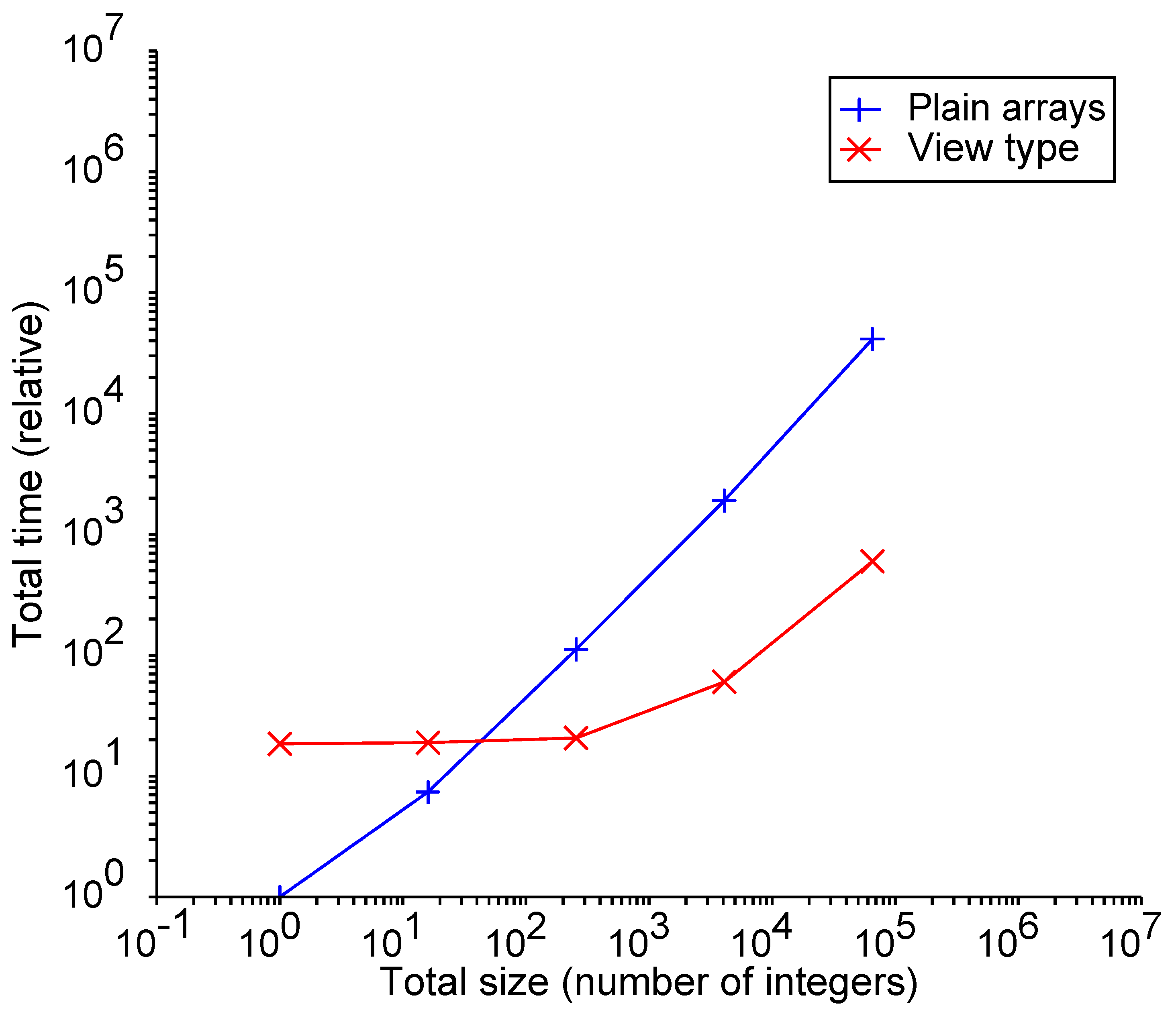
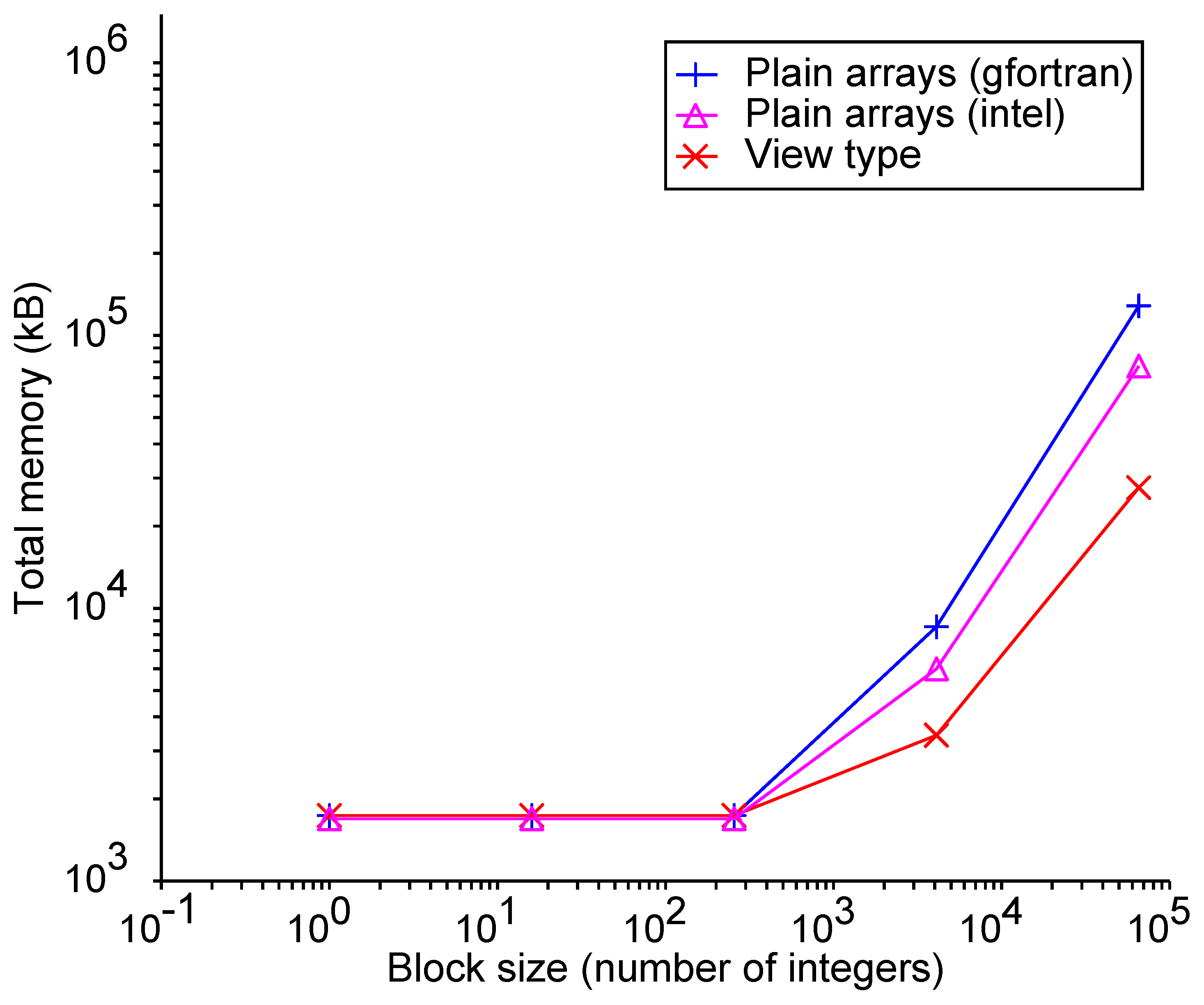
3.2. Experiment 1: Extending Arrays

Using the catenation operation for the moa_view_type variables, memory management only involves updating pointers to the various pieces of memory. No copying of the data is required.

This should make the catenation via the moa_view_type much more efficient (cf. Figure 1). Here, we catenate 100 memory blocks of ${16}^m$ integers (m = 0, 1, 2, 3, 4), using the standard Fortran facility and the specific MoA method. As can be seen from the graph, the MoA method is more efficient when the block size is more than 16 integers. The time required is essentially constant until the blocksize reaches 4096 integers ($m=3$). As the memory management of current-day computers is quite complex, the details of that management in combination with the access patterns in the program are likely to influence the form of both curves.

Our experiments did not explore how to prefetch addresses into caches through compiler flags and/or pragmas. We certainly would obtain a better performance if we used them and the compiler complied. Moreover, it would be better if we employed “dimension lifting” in the compiler so that, based on cache size, matrix size, and memory addresses, prefetching and buffering would be used. There are many optimizations that MoA can explore based on the speeds and sizes of arrays by breaking up loops. The size of the chunks would be part of the partitioning to bring in ideal cache sizes with prefetching up and down the memory hierarchy. Thus, a loop could be broken into two or more loops based on where the addresses are.

A second aspect that we examined was the memory use (Figure 2). Via the system routine getrusage(), it is possible to measure a large number of resource parameters within a running program (process), among which the maximum amount of memory can be used. As can be seen in the figure, this amount is constant and identical for the two implementations up to a blocksize of 4096 integers (16 kB, as each integer is four bytes). The minimum memory size is due to the program code and stack, as it is also measured for a version that merely starts and does not allocate anything.

The maximum allocated size in the program is $4\times 100\times \text{65,536}$ bytes or 25.6 MB. This is actually seen in the MoA version (“view type” in the figure), but for the version with plain arrays, the reported size is 4.6 times larger than for the view-type version for the gfortran compiler, version 11.3.0. This is unexpected; a factor of two or perhaps three, depending on how the implementation exactly works, was expected. The same ratio occurs with a blocksize of 4096 integers. The Intel Fortran oneAPI compiler, version 22.1.0, shows a factor of 3 between the actual maximum amount of memory used versus the maximum allocated size.

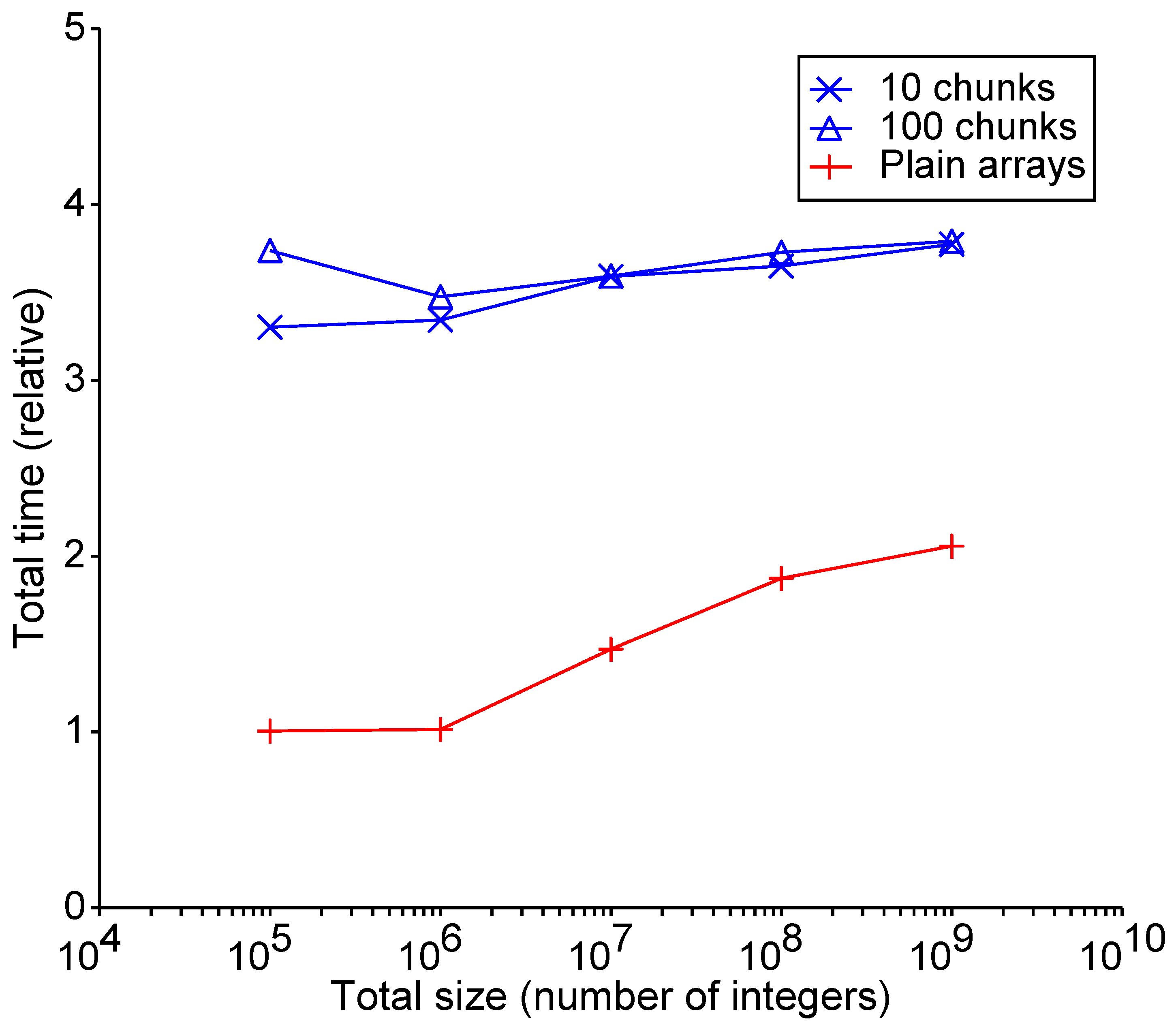
3.3. Experiment 2: Accessing Array Elements

Since we wanted the collection of catenated arrays to work in much the same way as ordinary arrays, but with the benefits of small blocks of memory, we looked at the performance of the two approaches in a single stylized case: summing selected elements of the arrays in an explicit loop.

  do i = 1,number_seq
      j = 1 + mod((i − 1) ∗ step, sz )
      subtotal = subtotal + x%elem(j)
  enddo
  total = total + mod(subtotal, 2)

In this experiment, a number of such loops were used with the intent to obtain a more or less realistic picture of typical array access patterns. Different strides (step in the code fragment) were used, and in one case, random array elements were selected. The non-unit strides and the random indices caused different access patterns and therefore different interactions with the caching mechanisms, which could be augmented by proper fetching.

Care must be taken, though:

• The work conducted in the loop must be large enough to let a measureable amount of time pass. Otherwise, noise will contaminate the results.
• The loops were repeated several thousands times to obtain a stable result, and even then, the measurements may have been influenced by whatever function the machine was performing at the time. So, the results presented here are the average of 30 individual runs.
• Optimizing compilers needed to be fooled; we were not interested in the result of the calculation, but the compiler may have noticed this and therefore “optimized away” the loop. For this reason, the result (total) was written to an external file.
• The “array” version and the “view” version should perform the same work for the timing results to be comparable. This is also applicable for compiler options (optimization and others).

The first versions of the moa_view_type class were ten times slower than the plain array version, which was a trifle disappointing. Analysis of the code and experimentation led to an implementation that was only two to three times slower: removing explicit range checking (akin to array bound checking) and caching whichever array segment the index was found in so that it could be used for the next access and other details. The results are shown in Figure 3.

As can be seen, the total run time was more or less constant for the two catenation experiments, whereas with the plain arrays, the run time grew steadily. For the lower range of the total size, there was a difference in timing with the MoA method. In the case of 10 chunks, the individual chunks were fairly large and, thus, accessing the array elements with a stride (step in the code fragment) more frequently hit the same chunk than in the case of 100 chunks. If the chunks were large enough, the overhead of finding the new chunk and loading it into the working memory became small in relation to the total time spent for each chunk.

An advantage of using chunks instead of a plain array is that there need not be a single large block of memory to store the data, but currently, their implementation is slower than that of plain arrays.

4. Conclusions and Further Steps

One of the advantages of MoA is that algorithms can be expressed without attention to low-level details. These can be suitably left to an almost mechanical translation step. Functional programming languages like LISP and Haskell present similar high-level approaches but are usually not geared towards arrays as primary data structures, which abound in the realm of numerical modeling and high-performance computing. Even machine learning relies intensely on the manipulation of vectors, matrices, and tensors.

Formulating the algorithms in this way allows compilers to take advantage of the compact notation and the finite set of operations to provide optimal implementations. In many ways, this is already achieved within the Fortran language via the set of intrinsic functions and the array operations. The philosophy of Mathematics of Arrays is, of course, not limited to Fortran. Many programming languages emphasize arrays as an important data structure. For instance, for C++, the Boost collection of libraries offers facilities to make working with arrays easier. The Julia programming language, in turn, defines different classes of arrays as part of its base language (cf. https://www.boost.org/ (accessed on 23 November 2024) and https://julialang.org/ (accessed on 23 November 2024)). Applying the ideas of MoA to these languages would enable a more or less language-agnostic development of useful algorithms.

For several algorithms, such as matrix multiplication and fast Fourier transforms, among others, Grout and Mullin discuss the application of MoA and the adaptation of the actual implementation of specialized hardware [8]. This shows the advantage of the abstract formulation via MoA of such algorithms.

In the specific context of Fortran, the advantage of intrinsic procedures over user-defined functions and subroutines are as follows:

• The programmer does not need to implement them themselves, something that may be quite non-trivial.
• The compiler knows the semantics exactly and can therefore decide on any number of optimizations and implementations. Typical libraries for linear algebra, like BLAS and LAPACK, have been highly optimized to take all possibilities into account with respect to memory layout and other machine-dependent characteristics. Such optimizations cannot be required from an individual programmer and are therefore limited to widely used libraries.

It is also possible for the compiler to hide the location of the data; instead of the programmer, the compiler, using MPI or OpenMP, decides that parallelism is possible and takes care of the data transfer to and from the available hardware (a cluster or GPUs). Such a transformation is easier when the semantics are described by MoA or Fortran array operations with a high-level notation.

A first step is the compiler being taught to recognize MoA operations to eliminate intermediate results. As a simple example, consider the following:

  C = matmul( transpose(A), B )

This does not require a temporary array storing the transpose of A, but it may be evaluated directly, because the effect of the functions matmul() and transpose() is known. Several features of the current Fortran standard, such as pure functions, which have no side effects, and the contiguous attribute for arrays and pointers to arrays, allow optimizations in this regard.

While compilers in general are large and very complex programs, the LFortran compiler [12] is open-source, is based on LLVM technology, and has been set up from the beginning to make experimentation possible.

The most important step now is to set up a research program into the full set of MoA functions and operations and their equivalent implementation in Fortran. This could result in an extension of the current library of intrinsic functions.

References

1. Berkling, K. Arrays and the Lambda Calculus; Technical Report 93, Electrical Engineering and Computer Science Technical Reports; Syracuse University: Syracuse, NY, USA, 1990. [Google Scholar]
2. Leiserson, C.E.; Thompson, N.C.; Emer, J.S.; Kusmaul, B.C.; Lampson, B.W.; Sanchez, D.; Schardl, T.B. There’s Plenty of Room at the Top: What will drive computer performance after Moore’s Law? Science 2020, 368, eaam9744. [Google Scholar] [CrossRef]
3. Backus, J.W. Can Programming Be Liberated From the von Neumann Style? A Functional Style and its Algebra of Programs. Commun. ACM 1978, 21, 613–641. [Google Scholar] [CrossRef]
4. Abrams, P.S. An APL Machine; Technical Report TR SLAC-114 UC-32(MISC); Stanford Linear Accelerator Center: Menlo Park, CA, USA, 1970. [Google Scholar]
5. Hassitt, A.; Lyon, L.E. Efficient Evaluation of Array Subscripts of Arrays. IBM J. Res. Dev. 1972, 16, 45–57. [Google Scholar] [CrossRef]
6. Mullin, L.M.R. A Mathematics of Arrays. Ph.D. Thesis, Syracuse University, Syracuse, NY, USA, 1988. [Google Scholar]
7. Mullin, L.R. Psi, the Indexing Function: A Basis for FFP with Arrays. In Arrays, Functional Languages, and Parallel Systems; Kluwer Academic Publishers: Dordrecht, The Netherlands, 1991. [Google Scholar]
8. Grout, I.A.; Mullin, L. Realizing Mathematics of Arrays Operations as Custom Architecture Hardware-Software Co-Design Solutions. Information 2022, 13, 528. [Google Scholar] [CrossRef]
9. Mullin, L.R.; Raynolds, J.E. Conformal Computing: Algebraically connecting the hardware/software boundary using a uniform approach to high-performance computation for software and hardware applications. arXiv 2008, arXiv:0803.2386. [Google Scholar]
10. ISO/IEC 1539-1:2023; Information Technology—Programming Languages—Fortran—Part 1: Base Language. ISO/IEC: Geneva, Switzerland, 2023. Available online: https://www.iso.org/standard/82170.html (accessed on 25 November 2024).
11. Reid, J. The new features of Fortran 2018. ACM SIGPLAN Fortran Forum 2018, 37, 5–43. [Google Scholar] [CrossRef]
12. Čertik, O. LFortran Compiler. 2022. Available online: https://lfortran.org/ (accessed on 25 November 2024).
Figure 1. Timings for extending plain arrays and moa_view_type variables. The total time for 100,000 iterations. The times are normalized to the time for the smallest plain arrays case and memory in the number of integers.
Software 03 00026 g001
Figure 2. Actual memory (in kB) used in the array extension experiment as a function of the blocksize (in the number of integers).
Software 03 00026 g002
Figure 3. Total run time for plain arrays and for catenated arrays, normalized by the smallest plain arrays case (moa_view_type).
Software 03 00026 g003
Disclaimer/Publisher’s Note: The statements, opinions and data contained in all publications are solely those of the individual author(s) and contributor(s) and not of MDPI and/or the editor(s). MDPI and/or the editor(s) disclaim responsibility for any injury to people or property resulting from any ideas, methods, instructions or products referred to in the content.